Permanent address ]
The Ginzburg-Landau Theory of Type II superconductors in magnetic field
Abstract
Thermodynamics of type II superconductors in electromagnetic field based on the Ginzburg - Landau theory is presented. The Abrikosov flux lattice solution is derived using an expansion in a parameter characterizing the ”distance” to the superconductor - normal phase transition line. The expansion allows a systematic improvement of the solution. The phase diagram of the vortex matter in magnetic field is determined in detail. In the presence of significant thermal fluctuations on the mesoscopic scale (for example in high materials) the vortex crystal melts into a vortex liquid. A quantitative theory of thermal fluctuations using the lowest Landau level approximation is given. It allows to determine the melting line and discontinuities at melt, as well as important characteristics of the vortex liquid state. In the presence of quenched disorder (pinning) the vortex matter acquires certain ”glassy” properties. The irreversibility line and static properties of the vortex glass state are studied using the ”replica” method. Most of the analytical methods are introduced and presented in some detail. Various quantitative and qualitative features are compared to experiments in type II superconductors, although the use of a rather universal Ginzburg - Landau theory is not restricted to superconductivity and can be applied with certain adjustments to other physical systems, for example rotating Bose - Einstein condensate.
I Introduction
Phenomenon of superconductivity was initially defined by two basic properties of classic superconductors (which belong to type I, see below): zero resistivity and perfect diamagnetism (or Meissner effect). The phenomenon was explained by the Bose - Einstein condensation (BEC) of pairs of electrons (Cooper pairs carrying a charge constant considered positive throughout) below a critical temperature . The transition to the superconducting state is described phenomenologically by a complex order parameter field with proportional to the density of Cooper pairs and its phase describing the BEC coherence. Magnetic and transport properties of another group of materials, the type II superconductors, are more complex. An external magnetic field and even, under certain circumstances, electric field do penetrate into a type II superconductor. The study of type II superconductor group is importance both for fundamental science and applications.
I.1 Type II superconductors in magnetic field
I.1.1 Abrikosov vortices and some other basic concepts
Below a certain field, the first critical field , the type II superconductor is still a perfect diamagnet, but in fields just above magnetic flux does penetrate the material. It is concentrated in well separated ”vortices” of size , the magnetic penetration depth, carrying one unit of flux
| (1) |
The superconductivity is destroyed in the core of a smaller width called the coherence length. The type II superconductivity refers to materials in which the ratio is larger than Abrikosov (1957). The vortices strongly interact with each other, forming highly correlated stable configurations like the vortex lattice, they can vibrate and move. The vortex systems in such materials became an object of experimental and theoretical study early on.
Discovery of high materials focused attention to certain particular situations and novel phenomena within the vortex matter physics. They are ”strongly” type II superconductors and are ”strongly fluctuating” due to high and large anisotropy in a sense that thermal fluctuations of the vortex degrees of freedom are not negligibly, as was the case in ”old” superconductors. In strongly type II superconductors the lower critical field and the higher critical field at which the material becomes ”normal” are well separated leading to a typical situation in which magnetic fields associated with vortices overlap, the superposition becoming nearly homogeneous, while the order parameter characterizing superconductivity is still highly inhomogeneous. The vortex degrees of freedom dominate in many cases the thermodynamic and transport properties of the superconductors.
Thermal fluctuations significantly modify the properties of the vortex lattices and might even lead to its melting. A new state, the vortex liquid is formed. It has distinct physical properties from both the lattice and the ”normal” metal. In addition to interactions and thermal fluctuations, disorder (pinning) is always present, which may also distort the solid into a viscous, glassy state, so the physical situation becomes quite complicated leading to rich phase diagram and dynamics in multiple time scales. A theoretical description of such systems is a subject of the present review. Two ranges of fields, and allow different simplifications and consequently different theoretical approaches to describe them. For large there is a large overlap of their applicability regions.
I.1.2 Two major approximations: the London and the homogeneous field Ginzburg - Landau models
In the fields range vortex cores are well separated and one can employ a picture of line-like vortices interacting magnetically. In this approach one ignores the detailed core structure. The value of the order parameter is assumed to be a constant with an exception of thin lines with phase winding around the lines. Magnetic field is inhomogeneous and obeys a linearized London equation. This model was developed for low superconductors and subsequently elaborated to describe the high materials as well. It was comprehensively described in numerous reviews and books Brandt (1995); Blatter et al. (1994); Kopnin (2001); Tinkham (1996) and will not be covered here.
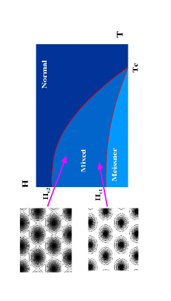
The approach however becomes invalid as fields of order of are approached, since then the cores cannot be considered as linelike and profile of the depressed order parameter becomes important. The temperature dependence of the critical lines is sketched in Fig. 1. The region in which the London model is inapplicable includes typical situations in high materials as well as in novel ”conventional” superconductors. However precisely under these circumstances different simplifications are possible. This is a subject of the present review.
When distance between vortices is smaller than (at fields of several ) the magnetic field becomes homogeneous due to overlaps between vortices. This means that magnetic field can be described by a number rather then by a field. This is the most important assumption of the Landau level theory of the vortex matter. One therefore can focus solely on the order parameter field . In addition, in various physical situation the order parameter is greatly depressed compared to its maximal value due to various ”pair breaking” effects like temperature, magnetic and electric fields, disorder etc. For example, in an extreme case of only small “islands” between core centers remain superconducting, yet superconductivity dominates electromagnetic properties of the material. One therefore can rely on expansion of energy in powers of the order parameter, a method known as the Ginzburg - Landau (GL) approach, which is briefly introduced next.
To conclude, while in the London approximation one assumes constant order parameter and operates with degrees of freedom describing the vortex lines, in the GL approach the magnetic field is constant and one operates with key notions like Landau wave functions describing the order parameter.
I.2 Ginzburg - Landau model and its generalizations
An important feature of the present treatise is that we discuss a great variety of complex phenomena using a single well defined model. The mathematical methods used are also quite similar in various parts of the review and almost invariably range from perturbation theory to the so called variational gaussian approximation and its improvements. This consistency often allows to consider a smooth limit of a more general theory to a particular case. For example a static phenomenon is obtained as a small velocity limit of the dynamical one, the clean case is a limit of zero disorder and the mean field is a limit of small mesoscopic thermal fluctuations. The model is motivated and defined below, while methods of solution will be subject of the following sections. The complexity increases gradually.
I.2.1 Landau theory near for a system undergoing a second order phase transition
Near a transition in which the phase symmetry, , is spontaneously broken a system is effectively described by the following Ginzburg-Landau free energy Mazenko (2006):
Here and we assumed equal effective masses in the plane , both possibly different from the one in the direction . This anticipates application to layered superconductors for which the anisotropy parameter can be very large. The last term, , the ”normal” free energy, is independent on order parameter, but might depend on temperature. The GL approach is generally an effective mesoscopic approach, in which one assumes that microscopic degrees of freedom are ”integrates out”. It is effective when higher powers of order parameter and gradients, neglected in eq.(I.2.1) are indeed negligible. Typically, but not always, it happens near a second order phase transition.
All the terms in eq.(I.2.1) are of order , where while one neglects (as ”irrelevant”) terms of order like and quadratic terms containing higher derivatives. Generally parameters of the GL model eq.(I.2.1) are functions of temperature, which can be determined by a microscopic theory or considered phenomenologically. They take into account thermal fluctuations of the microscopic degrees of freedom (”integrated out” in the mesoscopic description). Consistently one expands the coefficients ”near”, with coefficient vanishing at as :
| (3) | |||||
The second and higher terms in each expansion are omitted, since their contributions are also of order or higher. Therefore, when temperature deviates significantly from , one cannot expect the model to provide a good precision. Minimization of the free energy, eq.(I.2.1), with respect to below the transition temperature determines the value of the order parameter in a homogeneous superconducting state:
| (4) |
Substituting this into the last two terms in the square bracket in eq.(I.2.1), one estimates them to be of order , while one of the terms dropped, , is indeed of higher order. The energy of this state is lower than the energy of normal state with namely, by
| (5) |
is the condensation energy density of the superconductor at zero temperature.
The gradient term determines the scale over which fluctuations are typically extended in space. Such a length , called in the present context the coherence length, is determined by comparing the first two terms in the free energy:
| (6) |
So typically gradients are of order , and the first term in the free energy, eq.(I.2.1) is therefore also of the order . Since the order parameter field describing the Bose - Einstein condensate of Cooper pair is charged, minimal coupling principle generally provides an unambiguous procedure to include effects of electromagnetic fields.
I.2.2 Minimal coupling to magnetic field.
Generalization to the case of magnetic field is a straightforward use of the local gauge invariance principle (or the minimal substitution) of electromagnetism. The free energy becomes
while the Gibbs energy is
| (8) |
Here and we will assume that ”external” magnetic field (considered homogeneous, see above) is oriented along the positive axis, The covariant derivatives are defined by
| (9) |
The ”normal electrons” contribution is a part of free energy independent of the order parameter, but can in principle depend on external parameters like temperature and fields. Minimization with respect to and leads to a set of static GL equations, the nonlinear Schrödinger equation,
| (10) |
and the supercurrent equation,.
| (11) |
where the supercurrent and the ”normal” current
can be typically represented by the Ohmic conductivity and vanishes if the electric field is absent.
Comparing the second derivative with respect to term in eq.(11) with the last term in the supercurrent equation eq.(I.2.2), one determines the scale of typical variations of the magnetic field inside superconductor, the magnetic penetration depth:
| (13) |
This leads to
| (14) |
The two scales’ ratio defines the GL parameter . The second equation shows that supercurrent in turn is small since it is proportional to . Therefore magnetization is much smaller than the field, since it is proportional both to the supercurrent creating it and to . Since magnetization is so small, especially in strongly type II superconductors, inside superconductor and consistently disregard the ”supercurrent” equation eq.(11). Therefore the following vector potential
| (15) |
(Landau gauge) will be use throughout. The validity of this significant simplification can be then checked aposteriori.
I.2.3 Thermal fluctuations
Thermal fluctuations on the microscopic scale have already been taken into account by the temperature dependence of the coefficients of the GL free energy. However in high superconductors temperature can be high enough, so that one cannot neglect additional thermal fluctuations which occur on the mesoscopic scale. These fluctuations can be described by a statistical sum:
| (18) |
where a functional integral is taken over all the configurations of order parameter. In principle thermal fluctuations of magnetic field should be also considered, but it turns out that they are unimportant even in high materials Halperin et al. (1974); Dasgupta and Halperin (1981); Herbut and Tešanović (1996); Herbut (2007); Lobb (1987) .
Ginzburg parameter, the square of the ratio of to the superconductor energy density times correlation volume,
| (19) |
generally characterizes the strength of the thermal fluctuations on the mesoscopic scale Levanyuk (1959); Ginzburg (1960); Larkin and Varlamov (2005) and where . The definition of is the standard one as in Blatter et al. (1994) contrary to the previous definition used early in our papers, for example in Li and Rosenstein (2002a, 2003). Here is the coherence length in the field direction. The Ginzburg parameter is significantly larger in high superconductors compared to the low temperature one. While for metals this dimensionless number is very small (of order or smaller), it becomes significant for relatively isotropic high cuprates like () and even large for very anisotropic cuprate (up to ). Physical reasons behind the enhancement are the small coherence length, high and, in the case of large anisotropy . Therefore the thermal fluctuations play a much larger role in these new materials. In the presence of magnetic field the importance of fluctuations is further enhanced. Strong magnetic field effectively suppresses long wavelength fluctuations in direction perpendicular to the field reducing dimensionality of the fluctuations by two. Under these circumstances fluctuations influence various physical properties and even lead to new observable qualitative phenomena like the vortex lattice melting into a vortex liquid far below the mean field phase transition line.
Several remarkable experiments determined that the vortex lattice melting in high superconductors is first order with magnetization jumps Zeldov et al. (1995); Nishizaki et al. (2000); Willemin et al. (1998); Beidenkopf et al. (2005, 2007), and spikes in specific heat (it was found that in addition to the spike there is also a jump in specific heat which was measured as well) Schilling et al. (1996, 1997); Nishizaki et al. (2000); Bouquet et al. (2001); Lortz et al. (2006, 2007). These and other measurements like the resistivity and shear modulus point towards a need to develop a quantitative theoretical description of thermal fluctuations in vortex matter Pastoriza et al. (1994); Liang et al. (1996); Matl et al. (2002) To tackle the difficult problem of melting, the description of both the solid and the liquid phase should reach the precision level below 1% since the internal energy difference between the phases near the transition temperature is quite small.
I.2.4 Quenched Disorder.
In any superconductor there are impurities either present naturally or systematically produced using the proton or electron irradiation. The inhomogeneities both on the microscopic and the mesoscopic scale greatly affect thermodynamic and especially dynamic properties of type II superconductors in magnetic field. Abrikosov vortices are pinned by disorder. As a result of pinning the flux flow may be stopped and the material restores the property of zero resistivity (at least at zero temperature, otherwise thermal fluctuations might depin the vortices) and make various quantities like magnetization becomes irreversible. Disorder on the mesoscopic scale can be modeled in the framework of the Ginzburg - Landau approach adding a random component to its coefficients Larkin (1970). The random component of the coefficient of the quadratic term is called disorder, since it can be interpreted as a local deviation of the critical temperature from . The simplest such a model is the ”white noise” with local variance:
| (20) |
A dimensionless disorder strength , normalized to the coherence volume, is proportional to the density of the short range point - like pinning centers and average ”strength” of the center. The disorder average of a static physical quantity , denoted by in this case, is a gaussian measure
| (21) | |||||
The averaging process and its limitations is the subject of section IV, where the replica formalism is introduced and used to describe the transition to the glassy (pinned) states of the vortex matter. They are characterized by irreversibility of various processes. The quenched disorder greatly affects dynamics. Disordered vortex matter is depinned at certain ”critical current” and the flux flow ensues. Close to the flow proceeds slowly via propagation of defects (elastic flow) before becoming a fast plastic flow at larger currents. The I-V curves of the disordered vortex matter therefore are nonlinear. Disorder creates a variety of ”glassy” properties involving slow relaxation, memory effects etc. Thermal fluctuations in turn also greatly influence phenomena caused by disorder both in statics and dynamics. The basic effect is the thermal depinning of single vortices or domains of the vortex matter. The interrelations between the interactions, disorder and thermal fluctuations are however very complex. The same thermal fluctuations can soften the vortex lattice and actually can also cause better pinning near peak effect region . Critical current might have a ”peak” near the vortex lattice melting.
I.3 Complexity of the vortex matter physics
In the previous subsection we have already encountered several major complications pertinent to the vortex physics: interactions, dynamics, thermal fluctuations and disorder. This leads to a multitude of various ”phases” or states of the vortex matter. It resembles the complexity of (atomic) condensed matter, but, as we will learn along the way, there are some profound differences. For example there is no transition between liquid and gas and therefore no critical point. A typical magnetic () phase diagram advocated hereLi et al. (2006b) is shown on Fig. 2b. It resembles for example, an experimental phase diagram of high superconductor Divakar et al. (2004); Sasagawa et al. (2000) Fig. 2a.

Here we just mention various phases and transitions between them and direct the reader to the relevant section in which the theory can be found. Let us start the tour from the low and corner of the phase diagram in which, as discussed above, vortices form a stable Abrikosov lattice. Vortex solid might have several crystalline structures very much like an ordinary atomic solid. In the particular case shown at lower fields the lattice is rhombic, while at elevated fields in undergoes a structural transformation into a square lattice (red line on Fig. 2). These transitions are briefly discussed in section II. Thermal fluctuations can melt the lattice into a liquid (the ”melting” segment of the black line), section III, while disorder can turn both a crystal and a homogeneous liquid into a ”glassy” state, Bragg glass or vortex glass respectively (section IV). The corresponding continuous transition line (blue line on Fig.2) is often called an irreversibility line since glassiness strongly affects transport properties leading to irreversibility and memory effects.
To summarize we have several transition lines
1) The first order Zeldov et al. (1995); Schilling et al. (1996, 1997); Bouquet et al. (2001) melting line due to thermal fluctuations was shown to merge with the ”second magnetization peak” line due to pinning forming the universal order - disorder phase transition line Fuchs et al. (1998); Radzyner et al. (2002). At the low temperatures the location of this line strongly depends on disorder and generally exhibits a positive slope (termed also the ”inverse” melting Paltiel et al. (2000a, b)), while in the ”melting” section it is dominated by thermal fluctuations and has a large negative slope. The resulting maximum at which the magnetization and the entropy jump vanish is a Kauzmann point Li and Rosenstein (2003). This universal ”order - disorder” transition line (ODT), which appeared first in the strongly layered superconductors ( Fuchs et al. (1998)) was extended to the moderately anisotropic superconductors ( Radzyner et al. (2002)) and to the more isotropic ones like Li and Rosenstein (2003); Pal et al. (2001, 2002). The symmetry characterization of the transition is clear: spontaneous breaking of both the continuous translation and the rotation symmetries down to a discrete symmetry group of the lattice.
2) The ”irreversibility line” or the ”glass” transition (GT) line, which is a continuous transition Deligiannis et al. (2000); Taylor et al. (2003); Taylor and Maple (2007); Senatore et al. (2008).The almost vertical in the plane glass line clearly represents effects of disorder although the thermal fluctuations affect the location of the transition due to thermal depinning. Experiments in Fuchs et al. (1998); Beidenkopf et al. (2005, 2007) indicate that the line crosses the ODT line right at its maximum, continues deep into the ordered (Bragg) phase. This proximity of the glass line to the Kauzmann point is reasonable since both signal the region of close competition of the disorder and the thermal fluctuations effects. In more isotropic materials the data are more confusing. In Divakar et al. (2004); Sasagawa et al. (2000) the GT line is closer to the ”melting” section of the ODT line still crossing it. It is more difficult to characterize the nature of the GT transition as a ”symmetry breaking”. The common wisdom is that ”replica” symmetry is broken in the glass (either via ”steps” or via ”hierarchical” continuous process) as in the most of the spin glasses theories Fischer and Hertz (1991); Dotsenko (2001). The dynamics in this phase exhibits zero resistivity (neglecting exponentially small creep) and various irreversible features due to multitude of metastable states. Critical current at which the vortex matter starts moving is nonzero. It is different in the crystalline and homogeneous pinned phases.
3) Sometimes there are one or more structural transitions in the lattice phase Keimer et al. (1994); Gilardi et al. (2002); Johnson et al. (1999); McK. Paul et al. (1998); Divakar et al. (2004); Eskildsen et al. (2001); Sasagawa et al. (2000); Jaiswal-Nagar et al. (2006); Li et al. (2006a). They might be either first or second order and also lead to a peak in the critical current Chang et al. (1998a, b); Klironomos and Dorsey (2003); Park and Huse (1998); Rosenstein and Knigavko (1999).
I.4 Guide for a reader.
I.4.1 Notations and units
Throughout the article we use two different systems of units. In sections not dealing with thermal fluctuations, namely in section II and section IVA we use units which do not depend on ”external” parameters and , just on material parameters and universal constants (for example the unit of length is the coherence length ). More complicated parts of the review involving thermal fluctuations utilize units dependent on and . For example the unit of length in directions perpendicular to the field direction becomes magnetic length . However throughout the review basic equations and important results, which might be used for comparison with experiments and other theories, are also stated in regular physical units.
The mean field units and definitions of dimensionless parameters
Ginzburg - Landau free energy, eq.(I.2.1), contains three material parameters (in the directions perpendicular to the field and in the field direction respectively), . If in addition the disorder, introduced in eq.(20), is present, it is described by the disorder strength . These material parameters are usually expressed via physically more accessible lengths and time units .
| (22) |
Despite the fact that one often uses temperature dependent coherence length and penetration depth, which as seen in equation eqs.(6) and (13) might be considered as divergent near , we prefer to write factors of explicitly.
From the above scales can form the following dimensionless material parameters and
| (23) |
From the scales one can form units of magnetic and electric fields, current density and conductivity:
| (24) |
as well as energy density . These can be used to define dimensionless parameters, temperature magnetic and electric fields ,
| (25) |
from which other convenient dimensionless quantity describing the proximity to the mean field transition line are formed
| (26) |
The unit of the order parameter field (or square root of the Cooper pairs density) is determined by the mean field value :
| (27) |
and the Boltzmann factor and the disorder correlation in the physics units (length is in unit of in plane and in unit of along axis, order parameter in unit as defined by the equation above) is
The LLL scaled units
When dealing with thermal fluctuations, the following units depend on parameters and . Unit of length in directions perpendicular to the field can be conveniently chosen to be the magnetic length,
| (28) |
in the field direction, while in the field direction it is different:
| (29) |
Motivation for these fractional powers of both temperature and magnetic field will become clear in section III. we rescale the order parameter to by an additional factor:
| (30) |
Instead of or it will be useful to use ”Thouless LLL scaled temperature”:Thouless (1975); Ruggeri and Thouless (1976); Ruggeri (1978)
| (31) |
The scaled energy is defined by
| (32) |
and magnetization by
| (33) | |||||
The disorder is characterized by the ration of the strength of pinning to that of thermal fluctuations
| (34) |
I.4.2 Analytical methods described in this article
Discussion of properties of the GL model in magnetic fields utilizes a number of general and special theoretical techniques. We chose to describe some of them in detail, while others are just mentioned in the last section. We do not describe numerous results obtained using the elasticity theory or numerical methods like Monte Carlo and molecular dynamics simulations, although comparison with both is made, when possible.
The techniques and special topics include:
1) Translation symmetries in gauge theories (electro - magnetic translations) in IIA. Their representations, the quasi - momentum basis (IIIB) is used throughout to discuss excitations of vortex matter either thermal or elastic.
2) Perturbation theory around a bifurcation point of a nonlinear PDE (differential equations containing partial derivatives). This is very different from the perturbation theory used in linear systems, for example in quantum mechanics
3) Variational gaussian approximation to field theory Kleinert (1995) is widely used in III to IV. It is defined in IIIC in the path integral form and subsequently shown to be the leading order of a convergent series of approximants, the so called optimized perturbation series (OPE). The next to leading order, the post gaussian approximation, is related to the Cornwall -Jackiw -Tomboulis method is sometimes used, while higher approximants are difficult to calculate and are obtained to date for the vortex liquid only.
4) Ordinary perturbation theory in field theory is developed in the beginning of every section with enough details to follow. Spatial attention is paid to infrared (IR) and sometimes ultraviolet (UV) divergencies. We generally do not use the renormalization group (RG) resummation, except in subsection IIID, where it is presented in a form of Borel - Pade approximants.
5) Replica method to treat quenched disorder is introduced in IVB and used to describe the static and the thermodynamic properties of pinned vortex matter. Most of the presentation is devoted to the replica symmetric case, while more general hierarchial matrices are introduced in IVD following Parisi’s approach Parisi (1980); Mezard (1991).
Some technical details are contained in Appendix. We compare with available experiments on type II superconductors in magnetic field, while application or adaptation of the results to other fields in which the model can be useful (mentioned in summary) are not attempted..
I.4.3 Results
All the important results (in both regular physical units and the special units described above) are provided in a form of Mathematica file, which can be found on our web site.
II Mean field theory of the Abrikosov lattice
In this section we construct, following Abrikosov original ideas Abrikosov (1957), a vortex lattice solution of the static GL equations eq.(10) ”near” the line. In a region of the magnetic phase diagram in which the order parameter is significantly reduced from its maximal value , eq.(4), one does not really see well separated ”vortices” since, as explained in the previous section, their magnetic fields strongly overlap. Very close to even cores approach each other and consequently the order parameter is greatly reduced. Only small “islands” between the core centers remain superconducting. Despite this superconductivity dominates electromagnetic, transport and sometimes thermodynamic properties of the material. One still has a well defined ”centers” of cores: zeroes of the order parameter. They still repel each other and thereby organize themselves into an ordered periodic lattice.
To see this we first employ a heuristic Abrikosov’s argument, based on linearization of the GL equations and then develop a systematic perturbative scheme with a small parameter - the ”distance” from the line on the plane. The heuristic argument naturally leads to the lowest Landau level (LLL) approximation, widely used later to describe various properties of the vortex matter. The systematic expansion allows to ascertain how close one should stay from the line in order to use the LLL approximation. Having established the lattice solution, spectrum of excitations around it (the flux waves or phonon) are obtained in the next subsection. This in turn determines elastic, thermal and transport properties of vortex matter.
II.1 Solution of the static GL equations. Heuristic solution near
II.1.1 Symmetries, units and expansion in
Broken and unbroken symmetries
Generally, before developing (sometimes quite elaborate) mathematical tools to analyze a complicated model described by free energy eq.(I.2.1) and its generalizations, it is important to make full use of various symmetries of the problem. The free energy (including the external magnetic field) is invariant under both the three dimensional translations and rotations in the () plane. However some of the symmetries in the plane are broken spontaneously below the line. The symmetry which remains unbroken is the continuous translation along the magnetic field direction . As a result the configuration of the order parameter is homogeneous in the direction , . Hence the gradient term can be disregarded and the problem becomes two dimensional (here we consider the mean field equations only, when thermal fluctuations or point - like disorder are present the simplification is no longer valid.).
Units, free energy and GL equations
To describe the physics near it is reasonable to use the coherence length as a unit of length (assuming for simplicity ) and the value of the field at which the ”potential” part is minimal, eq.(4), (times ) will be used as a scale of the order parameter field
| (35) |
while the (zero temperature energy) density difference between the normal and the superconductor states of eq.(17) determines a unit of energy density. Therefore dimensionless 2D energy , where is the sample’s size in the field direction, and eq.(8) takes a form:
| (36) |
Dimensionless temperature and magnetic fields are and . The units of temperature and magnetic field are therefore and .
The linear operator is defined as
| (37) |
It coincides with the quantum mechanical operator of a charged particle in a constant magnetic field. The covariant derivative (with all the bars omitted from now on) is and the constant is defined as
| (38) |
It is positive in the superconducting phase and vanishes on the line, as will be shown in the next subsection. The reason why is ”shifted” by a constant compared to a standard Hamiltonian of a particle in magnetic field will become clear there. In rescaled units the GL equation takes a form:
| (39) |
The equation for magnetic field takes a form
| (40) |
with boundary condition involving the external field .
Expansion in powers of
In physically important cases one is encounters strongly type II superconductors for which . For example all the high cuprates have of order , and even low superconductors which are useful in applications have of order . In such cases it is reasonable to expand the second equation in powers of :
| (41) | |||||
It can be seen from eqs.(39) and (40) that to leading order in magnetic field is equal to the external field considered constant. Therefore one can ignore eq.(40) and use external field in the first equation. Corrections will be calculated consistently. For example magnetization will appear in the next to leading order.
From now on we drop bars over and consider the leading order in . Even this nonlinear differential equation is still quite complicated. It has an obvious normal metal solution , but might have also a nontrivial one. A simplistic way to find the nontrivial one is to linearize the equation. Indeed naively the nonlinear term contains the ”small” fields compared to one in the linear term. This assumption is problematic since, for example the coefficient of the term is also small, but will follow this reasoning nevertheless leaving a rigorous justification to subsection B.
II.1.2 Linearization of the GL equations near .
Naively dropping the nonlinear term in eq.(39), one is left with the usual linear Schröedinger eigenvalue equation of quantum mechanics for a charged particle in the homogeneous magnetic field
| (42) |
The Landau gauge that we use, defined in eq.(15), still maintains a manifest translation symmetry along the direction, while the translation invariance is “masked” by this choice of gauge. Therefore one can disentangle the variables:
| (43) |
resulting in the shifted harmonic oscillator equation:
| (44) |
where is the coordinate of the center of the classical Larmor orbital. For a finite sample is discretized in units of , while the Larmor orbital center is confined inside the sample leading to values of .
Nontrivial solutions of the linearized equation exist only for special values of magnetic field, since the operator has a discrete spectrum
| (45) |
for any (the Landau levels are therefore times degenerate). These fields satisfy
| (46) |
and the eigenfunctions are:
where are Hermit polynomials. As we will see shortly, the nonlinear GL equation eq.(39) acquires a nontrivial solution also at fields different from . The solution with (the lowest Landau level or LLL, corresponding to the highest ) appears at the bifurcation point
| (48) |
or . It defines the line.
For yet higher fields the only solution of nonlinear GL equations is the trivial one: . This is seen as follows. The operator is positive definite, as its spectrum eq.(45) demonstrates. Therefore for all three terms in the free energy eq. (36) are non - negative and in this case the minimum is indeed achieved by . For the minimum of the nonlinear equations should not be very different from a solution of the linearized equation at .
Since the LLL, , solutions
| (49) |
are degenerate, it is reasonable to try the most general LLL function
| (50) |
as an approximation for a solution of the nonlinear GL equation just below . However how should one chose the correct linear combination? Perhaps the one with the lowest nonlinear energy: the quartic term in energy eq.(36) will lift the degeneracy. Unfortunately the number of the variational parameters in eq.(50) is clearly unmanageable. To narrow possible choices of the coefficients, one has to utilize all the symmetries of the lattice solution. Therefore we digress to discuss symmetries in the presence of magnetic field, the magnetic translations, returning later to the Abrikosov solution equipped with minimal group theoretical tools.
II.1.3 Digression: translation symmetries in gauge theories
Translation symmetries in gauge theories
Let us consider a solution of the GL equations invariant under two arbitrary translations vectors. Without loss of generality one of them can be aligned with the axis. Its length will be denoted by . The second is determined by two parameters:
| (51) |
We consider only rhombic lattices (sufficient for most applications), which are obtained for . The angle between and is shown on Fig. 3. Flux quantization (assuming one unit of flux per unit cell) will be
| (52) |

Generally an arbitrary translation in the direction in the particular gauge that we have chosen, eq.(15), is very simple
| (53) |
where is the ”momentum” operator. Periodicity of the order parameter in the direction with lattice constant (in units of , as usual) means that the wave vector in eq.(49) is quantized in units of : and the variational problem of eq.(50) simplifies considerably:
| (54) | |||||
Periodicity with lattice vector is only possible only when absolute values of coefficients are the same and, in addition, their phases are periodic in .
Hexagonal lattice
In this case the basic lattice vectors are , see Fig. 3, . As a next simplest guess to construct a lattice configuration out of Landau harmonics one can try a two parameter Ansatz :
For the hexagonal (also called sometimes triangular) FLL . Geometry and the flux quantization gives us now which becomes (in rescaled units of )
| (56) |
We are therefore left again with just one variational parameter
Naive nonmagnetic translation in the ”diagonal” direction, see Fig. 3, now gives
| (58) |
This is again a “regauging”, which generally accompanies a symmetry transformation. The ”magnetic translation” now will be
| (59) |
The normalization is
| (60) |
which gives: . Combining the even and the odd parts, the normalized function also can be written in a form
| (61) | |||||
This form will be used extensively in the following sections.
General rhombic lattice
All the rhombic lattices with magnetic field are obtained from the Ansatz by assuming the phase :
| (62) |
The hexagonal lattice corresponds to , see Fig. 3. One can check that a rhombic lattice indeed is invariant under magnetic translations by and . The flux quantization takes a form
| (63) |
One notices ,and that generally we have a following relation,
| (64) |
where the right side equation is the solution in the case of and we replace by . There are of course infinitely many invariant functions differing by a ”fractional” translation as well as by rotation of the lattice. These symmetries are ”broken spontaneously” by the lattice. According to Goldstone theorem, they lead to existence of soft phonon modes in the crystalline phase and will be studied in section III.
General magnetic translations and their algebra
Let us generalize the discussion by considering an arbitrary Landau gauge. Using the experience with regauging of the two nontrivial translations in our gauge, which generally is defined a matrix
| (65) |
Magnetic translation operator for a general vector should be defined as
| (66) |
with a generator defined by
| (67) |
This can be derived using the general formula
| (68) |
valid when commutator is proportional to the identity operator. Applying the formula to the case of the expression eq.(66) with , and using the basic algebra one indeed obtains a number
| (69) |
The expression for magnetic translations can also be derived from a requirement that they commute with ”Hamiltonian” defined in eq.(37). In fact they commute with both covariant derivatives
| (70) |
as well. However, using the same basic algebra, one also observes that magnetic translations generally do not commute: differs from by a phase. This is a consequence of the Campbell-Baker-Hausdorff formula , which follows immediately from eqs.(68) and (69)
| (71) |
with the constant commutator given by . The group property therefore is
| (72) |
from which the requirement to have an integer number of fluxons per unit cell of a lattice follows:
| (73) |
Note that the generator of magnetic translations is not proportional to covariant derivative . The relation is nonlocal,
| (74) |
where is the antisymmetric tensor.
II.1.4 The Abrikosov lattice solution: choice of the lattice structure based on minimization of the quartic contribution to energy
The Abrikosov constant of a lattice structure
To lift the degeneracy between all the possible ”wave functions” with arbitrary normalization on the ground Landau level, one can try to minimize the quartic term in free energy eq.(36). It is reasonable to assume that more ”symmetric” configurations will have an advantage. In particular lattices will be preferred over ”chaotic” inhomogeneous ones. Moreover hexagonal lattice should be perhaps the leading candidate due to its relative isotropy and high symmetry. This configuration is preferred the in London limit Tinkham (1996) since vortices repel each other and try to self assemble into the most homogeneous configuration. A simpler square lattice was considered in fact as the best candidate by Abrikosov and we start from this lattice to try to fix the variational parameter . The energy constrained to the LLL is
| (75) |
The quartic contribution to energy density is proportional to the space average of which is called the Abrikosov :
In principle one can slightly generalize the method we used to calculate analytically both integrals and sums Saint-James et al. (1969), however will refrain from doing so here, since in Appendix A a more efficient method will be presented. The result is . More generally one it is shown there that for any lattice this constant is given by
| (77) |
where the summation is over the lattice sites . For example for for the hexagonal lattice.
Energy, entropy and specific heat
Free energy density of the leading order solution is indeed negative. Substituting a variational solution, one has
| (78) | |||
The FLL and the transition to the normal state can therefore described well by a ”dimensionally reduced” symmetric model with the complex ”order parameter” . It is similar to the Meissner state in the absence of magnetic field but in with the only difference being that between and (which is just about 10%). One minimizes it with respect to :
| (79) |
The average energy density at minimum (still on the subspace of square lattices) is given by
| (80) |
or, returning to the unscaled units, the energy density is
| (81) |
The first derivative with respect to temperature , the entropy density
| (82) |
smoothly vanishes at transition to the normal phase. On the other hand the second derivative, the specific heat divided by temperature, jumps to a constant
| (83) |
from zero in the normal phase. Note that in this section we use a simple GL model which neglects the normal state contribution to free energy, eq.(I.2.1), retaining only terms depending on the order parameter. The additional term is a smooth ”background”, also referred to as a ”contribution of normal electrons”.
Of course a similar argument is valid for any lattice symmetry with corresponding Abrikosov parameter . What is the correct shape of the vortex lattice? To minimize the energy in this approximation is equivalent to the minimization of with respect to shape of the lattice. This is achieved for the hexagonal lattice, although differences are not large. The square lattice incidentally has the largest energy among all the rhombic structures, some higher than that of the hexagonal lattice. This sounds rather small, but for a comparison, the typical latent heat at melting (difference in internal energies between lattice and homogeneous liquid) is of the same order of magnitude.
Magnetization to leading order in
Magnetization can be obtained via minimization of the Gibbs free energy with respect to magnetic induction In our units and within LLL approximation one can differentiate eq.(75) and the Maxwell term with respect to :
| (84) |
The magnetization is therefore proportional to the superfluid density and is thus highly inhomogeneous. Its space average is
| (85) |
For large (typical value for high superconductors is ) the magnetization is of order compared to and therefore negligible. This justifies an assumption of constant magnetic induction, which can be slightly corrected:
| (86) |
Rescaling back to regular units, one has
| (87) |
with
| (88) |
valid up to corrections of order .
A general relation between the current density and the superfluid density on LLL
The pattern of supercurrent flow around vortex cores can be readily obtained by substituting the Abrikosov vortex approximation into the expression for the supercurrent density eq.(I.2.2). We derive here a general relation between an arbitrary static LLL function eq.(50) and the supercurrent. It will be helpful for understanding of the mechanism behind the flux flow, occurring in dynamical situations, when electric field is able to penetrate a superconductor. The covariant derivatives acting on the LLL basis elements give:
| (89) | |||||
The covariant derivatives, which are linear combinations of ”raising” and ”lowering” Landau level operators,
| (90) | |||||
therefore raise an LLL function to the first LL. One can check that the following relation is valid:
| (91) |
where is the antisymmetric tensor. We therefore have established an exact relation between the current density and (scaled with according to eq.(24)) superfluid density,
| (92) |
valid, however, on LLL states only. In regular units the current density is related to (unscaled) order parameter field by
| (93) |
The supercurrent indeed creates a vortex around a dip in the superfluid density, Fig.4. The overall current is of course zero, since the bulk integral is transformed into a surface one.

An approximate solution described in this subsection is perhaps valid ”near” the line, however to estimate the range of validity and to obtain a better approximation, one would prefer a systematic perturbative scheme over an uncontrollable variational principle. This is provided by the expansion.
II.2 Systematic expansion around the bifurcation point.
II.2.1 Expansion and the leading order
We have defined the operator in eq.(37) in such a way that its spectrum will start from zero. This allows the development of the bifurcation point perturbation theory for the GL equation eq.(39). This type of the perturbation theory is quite different from the one used in linear equations like Schrödinger equation.
One develops a perturbation theory in small around the line :
| (94) |
Note the fractional power of the expansion parameter in front of the ”regular” series. This is related to the mean field critical exponent for a type equation being , so that all the terms in the free energy have the same power and are ”relevant”, as we mentioned in Introduction. Substituting this series into eq.(39) one observes that the leading () order equation gives the lowest LLL restriction already motivated in the heuristic approach of the previous subsection:
| (95) |
resulting in with normalization undetermined. It will be determined by the next order. The next to leading () order equation is:
| (96) |
Multiplying it with and integrating over coordinates, one obtains
| (97) |
The first term vanishes since Hermitian operator in the scalar product, defined as
II.2.2 Higher orders corrections to the solution
Next to leading order
Higher order corrections would in principle contain higher Landau level eigenfunctions in the basis of solutions of the linearized GL equation eq.(42) for eigenvalues , eq.(II.1.2). As on the LLL for higher Landau levels one can combine them into a lattice with a certain (here hexagonal) symmetry:
| (100) | |||||
The coefficients are the same as given in the previous subsection, eq.(II.1.3).
The order correction can be expanded in the Landau levels basis, eq.(100) as
| (101) |
(to simplify notations the LLL coefficient is denoted simply rather than , suppressing , the convention we have been using already for ). Inserting this into eq.(96), one obtains to order :
| (102) |
The scalar product with determines :
| (103) |
where
| (104) |
To find we need in addition also the order equation:
| (105) |
Inner product with gives:
| (106) |
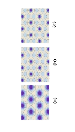
The expansion can be relatively easily continued. Fig. 5 shows three successive approximation. The convergence is quite fast even as far from the line at for .
Orders and in the expansion of free energy.
The mean field expression for the free energy to order was obtained already using heuristic approach, eq.(80).. Inserting the next correction eqs.(106) and (103) into eq.(36) one obtains the free energy density:
where is the unit of energy density.
It is interesting to note that only when , where is an integer. This is due to hexagonal symmetry of the vortex lattice Lascher (1965). For it decreases very fast with : Because of this the coefficient of the next to leading order is very small (additional factor of in the denominator). We might preliminarily conclude therefore that the perturbation theory in works much better that might be naively anticipated and can be used very far from transition line. If we demand that the correction is smaller then the main contribution the corresponding line on the phase diagram will be . For example the LLL melting line corresponds to . This overly optimistic conclusion is however incorrect as calculation of the following term shows.
How precise is LLL?
Now we discuss in what region of the parameter space the expansion outlined above can be applied. First of all note that all the contributions to are proportional to . This is a general feature: the actual expansion parameter is . One can ask whether the expansion is convergent and, if yes, what is its radius of convergence. Looking just at the leading correction and comparing it to the LLL one gets a very optimistic estimate. For this purpose higher orders coefficients were calculated Li and Rosenstein (1999a). The results for the are following:
| (108) | |||
and
| (109) | |||
where
| (110) |
We already can see that and are proportional to and in addition there is a factor of . Since, due to hexagonal lattice symmetry all the , vanish, so do . We have checked that there is no more small parameters, so we conclude that the leading order coefficient is much larger than first (factor ), but the second is only times larger than the third. The correction to free energy density is
| (111) |
Accidental smallness by factor of the coefficients in the expansion due to symmetry means that the range of validity of this expansion is roughly or . Moreover additional smallness of all the HLL corrections compared to the LLL means that they constitute just several percent of the correct result inside the region of applicability. To illustrate this point we plot on Fig. 5 the perturbatively calculated solution for . One can see that although the leading LLL function has very thick vortices (Fig. 5a), the first nonzero correction makes them of order of the coherence length (Fig. 5b). Following correction of the order makes it practically indistinguishable from the numerical solution. Amazingly the order parameter between the vortices approaches its vacuum value. Paradoxically starting from the region close to the perturbation theory knows how to correct the order parameter so that it looks very similar to the London approximation (valid only close to ) result of well separated vortices.
We conclude therefore that the expansion in works in the mean field better that one can naively expect.
III Thermal fluctuations and melting of the vortex solid into a liquid
In this section a theory of thermal fluctuations and of melting of the vortex lattice in type II superconductors in the framework of Ginzburg - Landau approach is presented. Far from the lowest Landau level approximation can be used. Within this approximation the model simplifies and results depend just on one parameter: the LLL reduced temperature. To obtain an accurate description of both the vortex lattice and the vortex liquid different methods are applied. In the crystalline phase basic excitations are phonons. Their spectrum and interactions are rather unusual and the low temperature perturbation theory requires to develop a certain technique. Generally perturbation theory to the two loop order is sufficient, but for certain purposes (like finding a spinodal in which metastable crystalline state becomes unstable) a self consistent ”gaussian” approximation is required. In the liquid state both the perturbation theory and gaussian approximations are insufficient to get a precision required to describe the first order melting transition and one utilizes more sophisticated methods. Already gaussian approximation shows that the metastable liquid state persists (within LLL) till zero temperature. The high temperature renormalized series (around the gaussian variational state) supplemented by interpolation to a metastable ”perfect liquid” state are sufficient. The melting line location is determined and magnetization and specific heat jumps along it are calculated. The magnetization of liquid is larger than that of solid by 1.8% irrespective of the melting temperature, while the specific heat jump is about 6% and decreases slowly with temperature.
III.1 The LLL scaling and the quasi - momentum basis
III.1.1 The LLL scaling
Units and the LLL scaled temperature
If the magnetic field is sufficiently high, we can keep only the LLL modes. This is achieved by enforcing the following constraint,
| (112) |
where covariant derivatives were defined in eq.(9). Using it the free energy eq.(8) simplifies:
| (113) | |||||
Originally the Ginzburg - Landau statistical sum, eq.(18), had five dimensionless parameters, three material parameters and the Ginzburg number, defined by
| (114) |
and two external parameters and . However, since there is now no gradient term in directions perpendicular to the field, it is missing one independent parameter. The Gibbs energy,
| (115) |
thus possesses the ”LLL scaling” Thouless (1975); Ruggeri and Thouless (1976); Ruggeri (1978); Lee and Shenoy (1972). To exhibit these scaling relations, it is useful to use units of coordinates and fields, which are dependent not just on material parameters (as those used in section II), but also on external parameters, magnetic field and temperature. One uses the magnetic length rather than coherence length as a unit of length in directions perpendicular to magnetic field, , while in the field direction different factor is used, . Magnetic field is rescaled as before with , while the order parameter field has an additional factor: . The usefulness of the fractional powers additional factors will become clear later.
The dimensionless Boltzmann factor becomes
| (117) |
where the LLL scale ”temperature” is
| (118) |
The constant was defined in eq.(38) and extensively used in the previous section. The scaled temperature therefore is the only remaining dimensionless parameter in eq.(III.1.1) in addition to the coefficient of the last term. Factors of in definition of ”dimensionless free energy” in eq.(III.1.1) are traditionally kept and will appear frequently in what follows. Assuming nonfluctuating constant magnetic field, one can disregard the last term in eq.(III.1.1), and consider the thermal fluctuations of the order parameter only. This assumption is typically valid in almost all applications and will be discussed in subsection E. Certain physical quantities, the ”LLL scaled” ones, are functions of this parameter only. We list the most important such quantities below.
Scaled quantities
The scaled free energy density is:
| (119) |
where is the rescaled volume and is related to the free energy density in unscaled units by
| (120) |
Turning to magnetization, let us return to conventional units eq.(113) and neglect fluctuations of magnetic field (considered in Halperin et al. (1974); Dasgupta and Halperin (1981); Herbut and Tešanović (1996); Herbut (2007); Lobb (1987)). Within LLL magnetization in the presence of thermal fluctuations is determined from
| (121) |
Taking the derivative, one obtains
| (122) | |||||
where from now on denotes the thermal average. The magnetization on LLL is therefore proportional to the superfluid density
| (123) |
This motivates the definition of the LLL scaled magnetization proportional to ,
| (124) |
which is related to magnetization by
| (125) |
Consequently depends on only, the statement called ”the LLL scaling” proposed in Thouless (1975); Ruggeri and Thouless (1976); Ruggeri (1978); Tešanović et al. (1992); Tešanović and Andreev (1994). It has been experimentally demonstrated in numerous experiments.
The specific heat contribution due to the vortex matter is generally defined by . Usually, since the GL approach is applied near , one can replace by in the Boltzmann factor, leaving the temperature dependence just inside the coefficient of in eq.(113). In this case the normalized specific heat is defined as
| (126) |
where is the mean field specific heat of solid calculated in the previous section. Substituting , if very near phase transition temperature, we can put in the scaling factor in this case, we obtain:
| (127) |
Since the range of applicability of LLL can extend beyond vicinity of , especially at strong fields (since they depress order parameter), one should use a more complicated formula which does not utilize :
| (128) | |||||
It no longer possesses the LLL scaling.
III.1.2 Magnetic translations and the quasi - momentum basis
It is necessary to use the representations of translational symmetry in order to classify various excitations of both the Abrikosov lattice and a homogeneous state created when thermal fluctuations become strong enough. As we have seen in subsection IIB, presence of magnetic field makes the use of the translational symmetry a nontrivial task, due to the need to ”regauge”. Here we use an algebraic approach to construct the quasi - momenta basis and then to determine the excitation spectrum of the lattice and the liquid, which in turn determines its elastic and thermal properties.
The quasi - momentum basis
We motivated the definition of the magnetic translation symmetries eq.(66) by the property that they transform various lattices onto themselves. More formally the plane translation operators , eq.(66), represent symmetries since they commute with ”Hamiltonian” of eq.(37). Excitations of the lattice are no longer invariant under the symmetry transformations. This in particular means that we cannot longer consider the problem as two dimensional. However, as in the solid state physics, it is convenient to expand them in the basis of eigenfunctions of the generators of the magnetic translations operators defined in eq.(66) and simple translations in the field, , direction:
| (129) | |||||
with commutation relation eq.(72): . The tree dimensional quasi - momentum vector is denoted by . It is easy to construct these functions explicitly. On the Landau level the 2D quasi - momentum function is given by:
| (130) |
where for and for a given lattice symmetry was constructed in IIA. Here we will take the hexagonal lattice functions of eq.(100). Indeed
| (131) |
To write it explicitly, the most convenient form of the magnetic translation is that of eq.(66), which gives
| (132) |
Since is unitary, the normalization is the same as that of . On LLL in our gauge one has:
In the direction along the field one uses the usual momentum:
| (134) |
where, as before, we use the notation .
The values of the quasi - momentum cover a Brillouin zone in the plane. As usual, it is convenient to work in basis vectors of the reciprocal lattice, , with the basis vectors
| (135) |
The measure is
| (136) | |||||
Beyond LLL the quasi - momentum basis consists of Landau level ”wave functions” with quasi-momentum :
The construction is identical to LLL. Even in the homogeneous liquid state, which is obviously more symmetric than the hexagonal lattice, we find it convenient to use this basis:
| (138) |
Energy in the quasi - momentum basis
As was discussed in section II, the lowest energy configurations belong to LLL. There is an energy gap to any configuration, so it is reasonable that, for temperatures small enough, their contribution is small. Restricting the set of states over which we integrate to LLL
| (139) |
one has the Boltzmann factor , eq.(117), and other physical quantities via new variables . The first two terms in eq.(117,) are simple
| (140) | |||||
The quartic term is
with
| (142) |
calculated in Appendix A. Generally the expression is not very simple due to the so called ”Umklapp” processes since when four quasi - momenta involved We turn now to the first application of this basis: calculation of harmonic excitations spectrum of the vortex lattice.
III.2 Excitations of the vortex lattice and perturbations around it.
III.2.1 Shift of the field and the excitation spectrum
Shift of the field and diagonalization of the quadratic part
For negative and neglecting thermal fluctuations the minimum of energy is achieved by choosing one of the degenerate lattice solutions, the hexagonal lattice in our case. This was the main subject of the previous section. When thermal fluctuations are weak, one can expand in temperature around the mean field solution. The zero quasimomentum field is then shifted by the mean field solutions. In our new LLL units we therefore express the complex fields via two ”shifted” real fields (, ):
| (143) |
with value of the field found in section II in the LLL units being
| (144) |
Notations ”” and ”” indicate an analogy to optical and acoustic phonons in atomic crystals. The constants will be chosen later and will help to diagonalize the quadratic part of the free energy. Substituting this into the energy eqs.(140) and (III.1.2), one obtains a constant ”mean field” energy density of section II,
| (145) |
while the quadratic part is
| (146) | |||
where functions,
| (147) | |||||
are calculated and given explicitly in Appendix A. There is no linear term,since we shifted by the mean field solution.
The choice
| (148) |
eliminates the terms, diagonalizing :
| (149) |
The resulting spectrum is:epsilon_III
| (150) | |||||
The cubic and quartic terms describing the anharmonicities or interactions of the excitations (phonons) are
| (152) | |||
where
| (153) |
| (154) |
with defined in eq.(142).
Supersoft Goldstone (shear) modes
While the O mode is ”massive” even for small quasi - momenta, the A mode is a Goldstone boson resulting from spontaneous breaking of several continuous symmetries and is therefore ”massless”. The broken symmetries include the electric charge (magnetic) translations and rotations. Spectrum of Goldstone modes is typically ”soft” and quadratic in momentum. This is indeed the case, as far as the field direction is concerned, eq.(150), but the situation in the perpendicular directions is different Lee and Shenoy (1972); Eilenberger (1967).
We use expansion of the functions and , eq.(147), derived in Appendix A:
| (155) | |||||
with constants given in Appendix A, . The acoustic spectrum consequently has the following expansion at small momenta:
| (156) |
All the quadratic term cancel and the Goldstone bosons are ”supersoft”.
One can further investigate the structure of these supersoft modes and identify them with ”shear modes” Moore (1989, 1992); Zhuravlev and Maniv (1999, 2002). To conclude, there are many broken continuous symmetries (translations in two directions, rotations and the phase transformations, forming a rather uncommon in physics Lie group) leading to a single Goldstone mode. The commutators of the magnetic translations generators and the generator are (using the explicit form eq.(67)):
| (157) |
and form the so called Heisenberg - Weyl algebra. However the Goldstone mode is much softer than the regular one: instead of . The situation is not entirely unique, since ferromagnetic spin waves, Tkachenko modes in superfluid and excitations in 2D electron gas within LLL share this property. A rigorous general derivation of the modification of the Goldstone theorem in this case is still not available. Note also that, when the magnetic part is not neglected, the modes become massive via a kind of Anderson - Higgs mechanism, which gives them a small ”mass” of order in our units.
This exceptional ”softness” apparently should lead to an instability of the vortex lattice against thermal fluctuations. Indeed naive calculation of the correlator in perturbation theory shows that certain quantities including superfluid density are infrared (IR) divergent Maki and Takayama (1971). This was even considered an indication that the vortex lattice does not exist Nikulov et al. (1995a); Nikulov (1995b); Moore (1997), despite large body of experimental evidence, even at that time. As a result, the perturbation theory around the Abrikosov solution was not developed beyond the one - loop order for a long time. One could argue Brandt (1995) that real physics is dominated by the small mass of the shear mode, acting as a cutoff that prevents IR divergencies, but basic physical properties related to thermal fluctuations near seemed to be independent of the cutoff, especially for high superconductors. In Rosenstein (1999) the IR divergencies were reconsidered and it was found that they all cancel exactly at each order in physical quantities like free energy, magnetization etc. We therefore systematically consider the (renormalized) perturbation theory for free energy up to two loops and then turn to other physical quantities.
III.2.2 Feynman diagrams. Perturbation theory to one loop.
Feynman diagrams for the loop expansion
To develop a perturbation theory, the coefficient in front of the Boltzmann factor, eq.(117) is considered large
| (158) |
The ”small parameter” is actually , but will be useful to organize the perturbation theory before the actual expansion parameter is uncovered in the process of assembling the series. One does not have to consider a linear in fields term since it involves only the Goldstone excitations and does not contribute to bulk energy density Jevicki (1977). The free energy is calculated from eq.(119) by expanding exponent of ”vertices” and , so that all the integrals become gaussian:
| (159) | |||
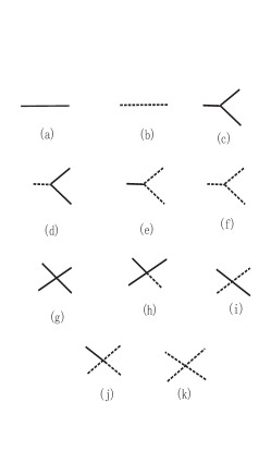
The propagators entering Feynman diagrams (Fig. 6a,b) are read from the quadratic part, eq.(140):
| (160) |
The leading order propagators are denoted by dashed and solid lines for the and the modes respectively. Nonquadratic parts of the free energy are the three - leg and the four - leg ”vertices”, Fig. 6c-f and Fig. 6g-k respectively. It is important for disappearance of ”spurious” IR divergencies (to be discussed later) to realize that vertices involving the field are ”soft”, namely at small momentum they behave like powers of . For example, the vertex, Fig. 6f, is very ”soft”. At small momenta it is proportional to the fourth power of momenta
The power of , , where are numbers of the three - leg and the four - leg vertices, in front of a contribution means that topologically the number of ”loops” is Itzykson and Drouffe (1991). The leading term, the mean field energy is of order .
Energy to the one loop order
Important point to note is that in the ”ordered” phase, despite the fact that we are talking about perturbation theory, the shift or, in other words, definition of the ”physical” excitation fields and in terms of the original fields can change from order to order Itzykson and Drouffe (1991). The shift in eq.(143) is therefore renormalized, that is,
| (161) |
One finds in the same way was found, namely, by minimizing the effective the free energy at the minimal order in which it appears. Let us therefore explicitly write several leading contributions to the energy
| (162) |
We us start from the ”mean field” part in eq.(159):
| (163) | |||
The leading order is and comes solely from the mean field contribution, which is therefore the leading contribution in eq.(159) and coincides with eq.(145):
| (164) |
This part of energy can also be viewed as an equation determining .
Substituting into the expression in the second square bracket in eq.(163) makes it zero. The only contribution to the order comes from the second term in eq.(159), the ”trace log”, equal to:
| (165) | |||
When we take the leading order in the expansion of the excitation spectrum in powers of
the one loop energy becomes:
| (167) |
III.2.3 Renormalization of the field shift and spurious infrared divergencies.
Energy to two loops. Infrared divergent renormalization of the shift
To order , corresponding to two loops, one has the first contribution from the mean field part, which contains , namely, the third square bracket in eq.(163). The ”trace log” term, eq.(165), contributes due to leading correction to the excitation spectrum eq.(III.2.2):
| (168) | |||||
while the rest of the contributions in eq.(159) are drawn as Feynman two - loop diagrams in fig.Fig. 7 and cannot contain , since propagators and vertices already provide one factor . The minimization with respect to results in:
Due to additional softness of the mode , the first (”bubble”) integral diverges logarithmically near :
| (170) |
This means apparently that for the infinite infrared cutoff fluctuations destroy the inhomogeneous ground state, namely the state with lowest energy is a homogeneous liquid. It is plausible that since the divergence is logarithmic, we might be at lower critical dimensionality in which an analog of Mermin - Wagner theorem Mermin and Wagner (1966); Itzykson and Drouffe (1991) is applicable. Even this does not necessarily means that perturbation theory starting from ordered ground state is uselessJevicki (1977). A rigorous way to proceed in these situations have been found while considering simpler models like the ” model”, , in with number of components larger then one, say . Considering the corresponding statistical sum, one first integrates exactly zero modes, existing due to spontaneous breaking of a continuous symmetry ( in our case, field rotations in the model) and then develops a perturbation theory via steepest descent method for the rest of the variables. When the zero mode (the above mentioned Goldstone boson with ) is taken out, there appears a single configuration with lowest energy and the steepest descent is well defined. For invariant quantities like energy this procedure simplifies: one actually can forget for a moment about integration over zero mode and proceed with the calculation, as if it is done in the ordered phase. The invariance of the quantities ensures that the zero mode integration trivially factorizes. This is no longer true for noninvariant quantities for which the machinery of ”collective coordinates method” should be used Rajaraman (1982).
In our case, we first note that the shift of the field is not a or translation invariant quantity, so invariant quantities like energy might be still calculable. Moreover the sign of the divergence is negative and a physically reasonable possibility that the shift decreases as a power of cutoff:
IR divergences in energy. The ”nondiagrammatic” mean field and Trlog contributions.
Substituting the IR divergent correction , eq.(III.2.3), back into the free energy, eqs.(163) and (168), one obtains a divergent contribution for the ”nondiagrammatic” terms in eq.(free_energy_expansion_III):
containing both the
| (173) |
and the sub leading divergences. However we haven’t finished yet with the order . They also likely to have divergences, naively even worse than logarithmic. We therefore return to the rest of contributions to the two loop order.
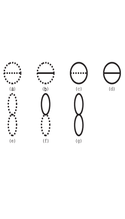
”Setting sun” diagrams.
One gets several classes of diagrams on Fig. 7, some of them IR divergent. The naively most divergent diagram fig.2a actually converges. It contains however two vertices, each one of them is proportional to the fourth power of momenta. The integrals over and can be explicitly performed using a formula
| (174) |
The divergences appear, when one or more factors in denominator belong to the mode for which for small . However, if the numerator vanishes at these momenta, the diagram is finite. The numerators contains vertices involving the same ”supersoft” field and typically vertices in theories with spontaneous symmetry breaking are also soft (this fact is known in field theoretical literature as ”soft pions” theorem due to their appearance in particle physics). In the present case they are ”super soft”. The vertex function, eq.(154), is
| (175) | |||
One easily sees that for each of the ”dangerous” momenta or each one of two vertices vanishes. For example when
| (176) | |||
This means that there are at least two powers of in the numerator and the integral converges. There are no other power-wise divergencies left to the two loop order. Analogous analysis of the vertex shows that the setting sun diagram, Fig. 7c is also convergent.
Naively logarithmically divergent setting sun diagram, Fig. 7b actually has both the and the divergences. The vertex function is
| (177) | |||
We will need its asymptotic when one of the momenta of the soft excitation is small
The leading divergence is determined by the asymptotics of the integrand as both and approach zero. Consequently it is given by the integral when the two vertex functions replaced with their values taken at and momenta of and in the denominator also taken to zero. The divergent part near is therefore
| (180) | |||||
The ”bubble” diagrams and cancellation of the leading divergences
Diagrams given in Figs .7e,f,g, can be easily evaluated:
| (181) | |||||
The leading divergence is
| (182) |
One observes that sum of three leading divergences given in eqs. (173), (180) and (182) cancel. There are still sub leading divergences. They require more care, since ”not dangerous” momenta cannot be put to zero, and are treated next.
Cancellation of the IR divergencies
The two - loop contribution to energy in a ”standard” form:
| (183) |
In order to demonstrate cancelation of the IR divergences we investigate the value of the numerator at and and show that and . The part due to nondiagrammatic terms eq.(III.2.3) can be written as:
| (184) | |||
similarly, the setting sun diagram,
| (185) |
according to eq.(180). The divergent part of the bubble diagrams can be written as:
| (186) |
One explicitly observes that . The same happens . Therefore all the IR divergences, e.g. the and cancelled. Similar cancellations of all the logarithmic IR divergencies occur in scalar models with Goldstone bosons in and (where the divergencies are known as ”spurious”Jevicki (1977); David (1981)).
Vortex lattice energy
The finite result for the Gibbs free energy to two loops (finite parts of the integrals were calculated numerically). Up to two loops the calculationLi and Rosenstein (2002a, b, c) (extending the one carried in ref.Rosenstein (1999) to Umklapp processes) gives:
| (187) |
In regular units the free energy density is
| (188) |
Below we use this expression to determine the melting line and various thermal and magnetic properties of the vortex solid: magnetization, entropy, specific heat. Near the melting point the precision becomes of order 0.1% allowing comparison with the free energy of vortex liquid, which is much harder to get. Eventually the (asymptotic) expansion becomes inapplicable near the spinodal point at which the crystal is unstable due to thermal ”softening”. This is considered using gaussian approximation in subsection D.
III.2.4 Correlators of the phase and the structure function
Correlator of the phase and helicity modulus
The correlator of the order parameter is finite at all distances in the absence of thermal fluctuations
| (189) |
where is finite exhibiting the phase long range order in the vortex lattice (despite periodic modulation). However the order is expected to be disturbed by thermal fluctuations. Leading order perturbation theory gives an early indication of the loss of the order in directions perpendicular to the field. The leading correction consists of the correction to the shift , eq.(III.2.3) and sum of two propagators
| (190) | |||
One observes that the logarithmic divergences of the second and the third terms cancel, but that the correlator in the plane depends on the large distance as a log:
| (191) | |||
It is expected, that exactly as the expectation value dependence on IR cutoff, the actual correlator is not growing logarithmically, by rather decreasing as a power . This is an example of the Berezinsky - Kosterlitz - Thouless phenomenon Itzykson and Drouffe (1991). It appears however at rather high dimensionality . Note however that the LLL constraint (large magnetic fields) effectively reduce dimensionality, enhancing the role of thermal fluctuations.
In the direction parallel to the field the correlations are still long range. Indeed the helicity modulus is
| (192) | |||
Structure function. Definitions
The superfluid density correlator, defined by
| (193) |
quantifies spontaneous breaking of the translational and rotational symmetries only as in both locations the superfluid density is invariant under the gauge transformations. This is different from the phase correlator discussed in the previous subsection, which decays as a power as indicated by the IR divergences. As in the case of the phase correlations, it is easier to consider the Fourier transform of the correlator, the structure function. Since translational symmetry is not broken along the field direction, one can restrict the discussion to the lateral correlations and consider partial Fourier transform:
| (194) |
In this subsection the structure function is calculated to leading order in thermal fluctuations strength (harmonic approximation) within the LLL, namely neglecting higher corrections. We discuss these corrections later.
Structure function of the vortex crystal without thermal fluctuations.
Substituting the LLL mean field solution eq.(61) into the definition of structure function one obtains:
| (195) | |||||
where we made use of formulas in Appendix A and delta function peaks are located at vectors of the reciprocal lattice. The height of the peak decreases rapidly beyond the reciprocal magnetic length (which is our unit). When mesoscopic thermal fluctuations are significant, they might broaden the peaks far below the temperature at which the lattice becomes unstable (the spinodal point).
Leading order corrections to thermal broadening of Bragg peaks
The calculation of the structure function closely follows that of free energy. The correlator is calculated using the Wick contractions:
| (196) |
The leading order () term is the mean field part, eq.(195), while the first order term is the harmonic fluctuation part.
The fluctuation part contains corrections term , same in structure as the leading order but with (IR diverging) coefficient instead of and four contractions (diagrams):
| (197) | |||
Performing integrations and Fourier transforms using methods described in Appendix A the first two contribution are:
where and are the ”integer” and the ”fractional” parts of , in a sense for inside Brillouin zone and on the reciprocal lattice. The third term is
| (199) |
while the last is:
Cancellation of the infrared divergences
Although all of the four terms , and are divergent as any of the peaks is approached, , the sums and are not. We start with the first two:
| (201) |
where
| (202) |
When it can be shown that , thus , and . Hence it will cancel the singularity coming from . Thus approaches when , and approaches when . Similarly the sum of and is not divergent, although separately they are. Their sum is.
| (203) |
with
| (204) |
Supersoft phonons and the ”halo” shape of the Bragg peaks
The sum of all the four terms can be cast in the following form:
| (205) | |||
The results were comparedLi and Rosenstein (2002a) with numerical simulation of the LLL system in Sasik and Stroud (1995). For reciprocal lattice vectors close to origin the value of are:
Table 1
Values of with small .
The correction to the height of the peak at , , is quite small. The theoretical prediction has roughly the same characteristic saddle shape ”halos” around the peaks as in MC simulation ref. Sasik and Stroud (1995) and experiment Kim et al. (1999). Conversely, MC simulation result provides the nonperturbative evidence for small . In eq.(205), if we would get a contribution from the most singular term . This term will become constant when , and we will not get the same characteristic saddle shape ”halos” around the peaks as in ref. Sasik and Stroud (1995). Consequently the asymptotics for is crucial for such characteristic shape and thus the MC simulation result provides a nonperturbative evidence for it.
Magnetization profile
Another quantity which can be measured is the magnetic field distribution. In addition to constant magnetic field background there are magnetization corrections due to field produced by supercurrent. To leading order in magnetization is given by eq.(123). The superfluid density is calculated as in eq.(190):
| (206) |
Its Fourier transform can be easily calculated:
| (207) | |||||
Performing integrals, one obtains:
The function and constant appeared in eq.(204).
III.3 Basic properties of the vortex liquid. Gaussian approximation.
III.3.1 The high temperature perturbation theory and its shortcomings
The loop expansion
Unlike the perturbation theory in the crystalline state, in which various translational, rotational and gauge symmetries are spontaneously broken, the perturbation theory at high temperature is quite straightforward. One directly uses the quadratic and the quartic terms in the Boltzmann factor, eq.(117) as a ”large” part and a ”perturbation”
| (209) |
Again the ”parameter” is actually , but is regarded as small and the actual expansion parameter will become apparent shortly. The Feynman rules for a field , namely the propagator
| (210) |
and the four - point vertex are given on Fig. 8a,b respectively is defined in eq.(142). Since is a complex field, we use an arrow to indicate the ”orientation” of the propagator.
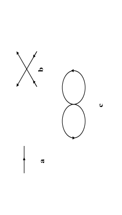
The leading contribution to the LLL scaled free energy, that of the quadratic theory, is
The in the last line is ultraviolet divergent, but unimportant for our purposes and will be generally suppressed. Corrections can be conveniently presented as Feynman diagrams.
The next, ”two - loop”, correction is the diagram in fig. 8c, which reads
Observe that the integrations can be reduced to corresponding integrations in quantum mechanics of the anharmonic oscillator Thouless (1975); Ruggeri and Thouless (1976); Ruggeri (1978), so that the series resemble a dimensionally reduced field theory or quantum mechanics.
Actual expansion parameter and the applicability range
This expansion can be carried to a high order after several simple tricks are learned Thouless (1975); Ruggeri and Thouless (1976); Ruggeri (1978); Hu and MacDonald (1993); Hu et al. (1994). The result to four loops is:
| (213) |
One observes that the small parameter is although coefficients grow and series are asymptotic. The difference with analogous expansion in the crystalline phase is that the sign of is opposite and the leading order is rather than . Phenomenologically the region of positive large is not very interesting since at that point, for example, magnetization is already very small. Also higher Landau levels effects become significant as will be discussed in subsection E, where HLL effects Prange (1969) are considered.
Therefore attempts were made to extend the series to smaller temperatures. One of the simplest methods is to perform a Hartree - Fock type resummation order by order. Let us first describe in some detail a certain variant of this type of approximation called generally gaussian, since it will be extensively used to treat thermal fluctuations as well as disorder effects in the following sections. It will be shown in subsection D that the approximation, is not just a variational scheme, but constitutes a first approximant in a convergent series of approximants (which however are not series in an external parameter) called ”optimized perturbation theory” (OPT).
III.3.2 General gaussian approximation
Variational principle
We start from the simplest, one parameter version of the gaussian approximation which is quite sufficient to describe the basic properties of the vortex liquid well below the mean field transition point . Within this approximation one introduces a variational parameter (which is physically an excitation energy of the vortex liquid) adding and subtracting a simple quadratic expression from the Boltzmann factor:
| (214) |
| (215) | |||||
where the constant was defined by
| (216) |
Now one considers as an ”unperturbed” part and as a small perturbation. This is a different partition than the one we used previously to develop a perturbation theory. Despite the fact that , we develop perturbation theory as before. To first order in the scaled free energy is:
| (217) | |||
where is the gaussian partition function and thermal averages denoted by are made in this quadratic theory.
Collecting terms, one obtains
| (218) |
Now comes the improvement. One optimizes the solvable quadratic large part by minimizing energy for with respect to . The optimization condition is called ”gap equation”,
| (219) |
since the BCS approximation is one of the famous applications of the general gaussian approximation.
Existence of a metastable homogeneous state down to zero temperature. Pseudocritical fixed point.
It is clear that the overheated solid becomes unstable at some finite temperature. It not clear however whether over - cooled liquid becomes unstable at some finite temperature (like water) or exists all the way down to as a metastable state. It was shown by variety of methods that liquid (gas) phase of the classical one component Coulomb plasma exists as a metastable state down to zero fluctuation temperature with energy gradually approaching that of the Madelung solid and excitation energy diminishing Leote de Carvalho et al. (1999). It seems plausible that the same would happen with any system of particles repelling each other with sufficiently long range forces. In fact the vortex system in the London approximation becomes a sort of repelling particles with the force even more long range than Coulombic.
Note that there always exists one solution of this cubic equation for positive for all values of , negative as well as positive. The excitation energy in the liquid decreases asymptotically as
| (220) |
at temperatures approaching zero. Importantly it becomes small at the melting point located at , see below. The gaussian energy is plotted on Fig. 9 (marked as the line).
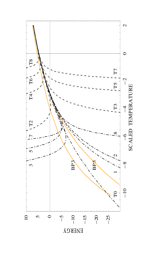
The existence of the solution means that the homogeneous phase exists all the way down to albeit as a metastable state below the melting point at which the free energy of the solid is smaller, see Fig. 11. Physically this rather surprising fact is intimately related to repulsion of the vortex lines. It is well known that if in addition to repulsion there exists an attraction like a long range attractive forces between atoms and molecules, they will lead to a spinodal point of the liquid Lovett (1977). However, if the attractive part is absent like in, for instance, electron liquid, one component plasma etc., the spinodal point is pushed down to zero temperature. It becomes a ”pseudocritical” point, namely, exhibits criticality, but globally unstable due to existence of a lower energy state Compagner (1974). Scaled LLL free energy density diverges as a power as well
| (221) |
see Fig. 9.
Assuming absence of singularities on the liquid branch allows to develop an essentially precise theory of the LLL GL model in vortex liquid (even including overcooled liquid) using the Borel - Pade (BP) Baker (1990) method at any temperature. This calculation is carried out in subsection D4. The gaussian liquid state can be used as a starting point of ”renormalized” perturbation theory around it. Such an expansion was first developed by Ruggeri and Thouless Thouless (1975); Ruggeri and Thouless (1976); Ruggeri (1978) for the GL model.
III.4 More sophisticated theories of vortex liquid.
III.4.1 Perturbation theory around the gaussian state
After the variational spectrum was fixed, one can expand in presumably small terms in eq.(214) multiplied by up to a certain order. Here we summarize the Feynman rules.
Feynman diagrams
The propagator in the quasi - momentum space,
| (222) |
is the same as in usual perturbation theory, Fig. 8a, but with gaussian mass . The four - leg interaction vertex is also the same as Fig. 8b, but there is an additional two - leg term. It has a factor and treated as a vertex and can be represented by a dot on a line, Fig. 10a, with a value of . The second term is a four line vertex, Fig. 8b, with a value of .
To calculate the effective energy density , one draws all the connected vacuum diagrams. To the three loop order one has:
| (223) | |||||
The liquid LLL (scaled) free energy is generally written as (using the gap equation)
| (224) |
The function can be expanded as
| (225) |
where the high temperature small parameter is . The coefficients which were calculated to order in Thouless (1975); Ruggeri and Thouless (1976); Ruggeri (1978) and extended to order in Brézin et al. (1990); Hikami et al. (1991). The consecutive approximants are plotted on fig.6 ( to ).
Applicability range and ways to improve it
One clearly sees that the series are asymptotic and can be used only at . Therefore the great effort invested in these high order evaluations still falls short of a required values to describe the melting of the vortex lattice. One can improve on this by optimizing the variational parameter at each order instead of fixing it at the first order calculation. This will lead in the following subsections to a convergent series instead of the asymptotic one. The radius of convergence happens to be around short of melting and roughly at the spinodal point of the vortex solid (see next subsection).
Another direction is to capitalize on the ”pseudocritical fixed point” at zero temperature. Indeed, the excitation energy, for example, behaves as a power other physical quantities are also ”critical”, at least according to gaussian approximation. It is therefore possible to consider supercooled liquid or liquid above the melting line but at low enough temperature as being in the neighborhood of a pseudocritical point. To this end the experience with critical phenomena is helpful. One generally develops an expansion around a weak coupling unstable fixed point (high temperature in our case) and ”flows” towards a strong coupling stable fixed point (zero temperature in our case) Itzykson and Drouffe (1991). Practically, when higher order expansions are involved, one makes use of the renormalization group methods in a form of the Pade - Borel resummation Baker (1990). This route will be followed in subsection 3 and will lead to a theory valid for arbitrarily low temperature. The OPE will serve as a consistency check on the upper range of applicability of the resummation, which is generally hard to predict.
III.4.2 Optimized perturbation theory.
General idea of the optimized gaussian perturbation theory
We will use a variant of OPT, the optimized gaussian series Kleinert (1995) to study the vortex liquidLi and Rosenstein (2001, 2002a, 2002b, 2002c). It is based on the ”principle of minimal sensitivity” idea Stevenson (1981); Okopinska (1987), first introduced in quantum mechanics. Any perturbation theory starts from dividing the Hamiltonian into a solvable ”large” part and a perturbation. Since we can solve any quadratic Hamiltonian we have a freedom to choose ”the best” such quadratic part. Quite generally such an optimization converts an asymptotic series into a convergent one (see a comprehensive discussion, references and a proof in Kleinert (1995)). The free energy is divided into the ”large” quadratic part and a perturbation introducing variational parameter like for gaussian approximation, eq.(214), although now the minimization will be made on orders of higher than the first.
Expanding the logarithm of the statistical sum to order
| (226) | |||
where denotes the sum of all the connected Feynman diagrams with as a propagator and then taking we obtain a functional of . To define the order OPT approximant one minimizes with respect to :
| (227) |
Till now the method has been applied and comprehensively investigated in quantum mechanics only (Kleinert (1995) and references therein) although attempts in field theory have been made Duncan and Jones (1993); Guida et al. (1995, 1996); Bender et al. (1994); Bellet et al. (1996a, b).
Implementation and the convergence radius in GL
We can obtain all the OPT diagrams which do not appear in the gaussian theory by insertions of bubbles and the additional vertex fig1c.insertions from the diagrams contributing to the non - optimized theory. Bubbles or ”cacti” diagrams, see Fig.8, are effectively inserted into energy by a technique known in field theory Kleinert (1995). One writes f in the following form:
| (228) |
where and is given by a solution of cubic equation
| (229) |
Summing up all the insertions of the mass vertex, which now has a value of is achieved by
| (230) |
We then expand f to order and then taking , to obtain . The solution of eq.(229) can be obtained perturbatively in :
| (231) |
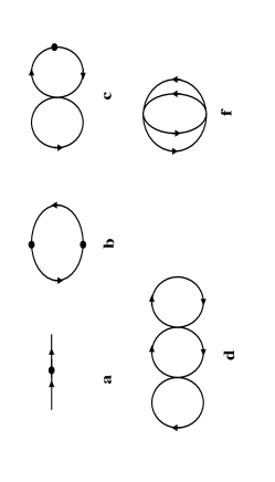
The nth OPT approximant is obtained by minimization of with respect to :
| (232) |
The above equation is equal to times a polynomial of order in . That eq.(232) is of this type can be seen by noting that the function f depends on combination only. We were unable to prove this rigorously, but have checked it to the order in This property simplifies greatly the task: one has to find roots of polynomials rather than solving transcendental equations. There are (real or complex) solutions for . However (as in the case of anharmonic oscillator Kleinert (1995)) the best root is the real root with the smallest absolute value,.
We then obtain solving the cubic equation, , explicitly:
For we obtain the gaussian result, dashed line marked ”T0” on Fig. 9.
Feynman rules undergo minor modifications. The mass insertion vertex, now has a value of , while the four line vertex is . However since the propagator in the field direction and perpendicular factorizes, the integrations can be reduced to corresponding integrations in quantum mechanics of the anharmonic oscillator, as we explained in subsection B. Expanding f in to order , then one then sets to obtain . We list here first few OPT approximants :
| (234) | |||||
with higher orders given in ref.Li and Rosenstein (2002b).
Rate of convergence of OPT
The remarkable convergence of OPE in simple models was investigated in numerous works Duncan and Jones (1993); Guida et al. (1995, 1996); Bender et al. (1994); Bellet et al. (1996a, b). It was found that at high orders the convergence of partition function of simple integrals (similar to the ”zero dimensional GL” studied in Wilkin and Moore (1993) ),
| (235) |
is exponentially fast. The reminder in bound by Duncan and Jones (1993); Guida et al. (1995, 1996); Bender et al. (1994); Bellet et al. (1996a, b)
| (236) |
For quantum mechanical anharmonic oscillator (both positive and negative quadratic term) it is just a bit slower:
| (237) |
where is the ground state energy. We follow here the convergence proof of Duncan and Jones (1993); Guida et al. (1995, 1996); Bender et al. (1994); Bellet et al. (1996a, b). The basic idea is to construct a conformal map from the original coupling to a coupling of bounded range and isolate a nonanalytic prefactor. Suppose we have a perturbative expansion (usually asymptotic, sometimes non Borel summable)
| (238) |
One defines a set of conformal maps dependent on parameter of coupling onto new coupling
| (239) |
While range of is the cut complex plane the range of is compact. The value of parameter for each approximant will be defined later. Then one defines a ”scaled” energy
| (240) |
where the prefactor is determined by strong coupling limit so that is bounded everywhere. Approximants to are expansion to th order in
| (241) |
with parameter substituted by . The energy approximant becomes
| (242) |
Two exponents and , for example, anharmonic oscillator and 3D GL model. OPE is equivalent to choosing which minimizes . It can be shown quite generally (see Appendix C of paper in Bender et al. (1994) and Kleinert (1995)) that the minimization equation is a polynomial one in . This is in line with our observation in the previous subsection that minimization equations are polynomial in with identified as
The remainder using dispersion relation is bounded by
| (243) |
where exponent is determined by discontinuity of at small negative :
| (244) |
The constants are for anharmonic oscillator and for 3D GL model Thouless (1975); Ruggeri and Thouless (1976); Ruggeri (1978). For 3D GL model, we found that as in anharmonic oscillator.
III.4.3 Overcooled liquid and the Borel - Pade interpolation
Borel - Pade resummation
We have already observed using the gaussian approximation that there exists a pseudo - critical fixed point at zero fluctuation temperature . One can therefore attempt to use the RG ”flow” from the weak coupling point, the perturbation at high temperature to this strongly couple fixed point. This procedure always have an element of interpolation. It should be consistent with the perturbation theory, but goes far beyond it. Technically it is achieved by the Borel - Pade (BP) approximants. We will not attempt to describe the method in detail, see textbooks Baker (1990), and concentrate on application.
The procedure is not unique. One starts from the renormalized perturbation series of , calculated in subsection B, eq.(225), . We will denote by the BP transform of (other BP approximants clearly violate the correct low temperature asymptotics and are not considered). The BP transform is defined as
| (245) |
where is the Pade transform of the better convergent series
| (246) |
The Pade transform of a function is defined as a rational function of the form
| (247) |
whose expansion up to order coincides with that of the function the series eq.(246).
The results are plotted on Fig. 9 as solid lines for and . The lines for are practically indistinguishable on the plot. The energy converges therefore, even at low temperatures below melting. It describes therefore the metastable liquid up to zero temperature. Due to inherent non - unique choice of the BP approximants it is crucial to compare the results with convergent series (within the range of convergence). This is achieved by comparison with the OPT results of the previous subsection.
Comparison with other results
As is shown on Fig. 9, the two highest available BP approximants are consistent with the converging OPT series described above practically in the whole range of . One can compare the results with existing (not very extensive) Monte Carlo simulation and agreement is well within the MC precision. Moreover similar method was applied to the 2D GL model which was simulated extensively Kato and Nagaosa (1993); Tešanović and Xing (1991); O’Neill and Moore (1993); Hu and MacDonald (1993); Hu et al. (1994) and for which longer series are available Brézin et al. (1990); Hikami et al. (1991) and agreement is still perfect. We conclude that the method is precise enough to study the melting problem.
Now let us mention several issues, which prevented its use and acceptance early on. Ruggeri and Thouless Thouless (1975); Ruggeri and Thouless (1976); Ruggeri (1978) tried to use BP to calculate the specific heat without much success because their series were too short Wilkin and Moore (1993). In addition they tried to force it to conform to the solid expression at low temperatures, which is impossible. Attempts to use BP for calculation of melting also ran into problems. Hikami, Fujita and Larkin Brézin et al. (1990); Hikami et al. (1991) tried to find the melting point by comparing the BP energy with the one loop solid energy and obtained . However their one loop solid energy was incorrect (by factor ) and in any case it was not precise enough, since the two loop contribution is essential.
To conclude the BP method and the OPT are precise enough to quantitatively determine thermodynamic properties of the vortex liquid, including the supercooled one. The precision is good enough in order to determine the melting line. We therefore turn to the physical consequences of the analytical methods for both the crystalline and the melted liquid states.
Magnetization and specific heat in vortex liquids
As long as the free energy is known, one differentiates it to calculated other physical quantities like entropy, magnetization and specific heat using general LLL formulas. Since the BP formulas, although analytical, are quite bulky (and can be found in Mathematica file) we will not provide them. The magnetization curves were compared to those in fully oxidized in Li and Rosenstein (2002a) to data of ref. Nishizaki et al. (2000) and with (after correction to a rather small ) to data of ref. Salem-Sugui et al. (2002), while the specific heat data were compared with experimental in in ref. Lortz et al. (2006) and in (also after the finite correction).
III.5 First order melting and metastable states
III.5.1 The melting line and discontinuity at melt
Location of the melting line
Comparing solid two - loop free energy given by eq.(188) and liquid BP energy, Fig. 11, we find that they intersect at (see insert for the difference). The available 3D Monte Carlo simulations Sasik and Stroud (1995) unfortunately are not precise enough to provide an accurate melting point since the LLL scaling is violated and one gets values ,, at magnetic fields ,, respectively. This is perhaps due to small sample size (100 vortices). The situation in 2D is better since the sample size is much larger. We performed similar calculation to that in 3D for the 2D LLL GL liquid free energy, combined it with the earlier solid energy calculation Rosenstein (1999); Li and Rosenstein (2002a)
| (248) |
and find that the melting point obtained . It is in good agreement with numerous MC simulations Hu and MacDonald (1993); Hu et al. (1994); Li and Nattermann (2003); Kato and Nagaosa (1993).

Comparison with phenomenological Lindemann criterion and experiments
Phenomenologically melting line can be located using Lindemann criterion or its more refined version using Debye - Waller factor. The more refined definition is required since vortices are not point - like. It was found numerically for Yukawa gas Stevens and Robbins (1993) that the Debye - Waller factor (ratio of the structure function at the second Bragg peak at melting to its value at ) is about . To one loop order one gets using methods of Li and Rosenstein (1999b) to calculate the Debye - Waller factor at the melting line obtained here by using the non-perturbative method
| (249) |
The higher loop correction to this factor is supposed to be positive and the total value might be equal to a value around (we did not undertake this calculation due to the complexity). However we apply a ”one loop” criterion (Debye - Waller factor is calculated to one loop), and this method was applied to the layered superconductor based on Lawrence- Doniach- Ginzburg Landau model and the rotating Bose Einstein condensate in Feng et al. (2009); Wu et al. (2007), and the results were both in surprisingly good agreements with numerical calculations in Hu and MacDonald (1997); Cooper et al. (2001).
The melting line in accord with numerous experiments in both clean low materials like Kokubo et al. (2004, 2005); Xiao et al. (2004); Adesso et al. (2006); Thakur et al. (2005); Kokubo et al. (2007) and Lortz et al. (2006), in which the line can be inferred from the peak effect (see below) and various dynamical effects or high like the fully oxidized Nishizaki et al. (2000), see fit in Li and Rosenstein (2002a). The fully oxidized is best suited for the application of the present theory, since pinning on the mesoscopic scale is negligible. For example the melting line is extended beyond as shown in Li and Rosenstein (2002a).
Melting lines of optimally doped untwined Schilling et al. (1996, 1997); Bouquet et al. (2001); Welp et al. (1991, 1996); Willemin et al. (1998) and Roulin et al. (1996a, b); Revaz et al. (1998) are also fitted extremely wellLi and Rosenstein (2003). More recently both and thick films of were fitted in ref. Kokubo et al. (2007) in which disorder is significant, but the pristine melting line is believed to be clearly seen in dynamics via peak effect. In Table 2 parameters inferred from these fits are given where the data for , , are taken from Schilling et al. (1996), Nishizaki et al. (2000), Roulin et al. (1996a) respectively. Parameters like characterizing the strength of thermal fluctuations differ a bit from the often mentioned Blatter et al. (1994). Similar fits were made in 2D for organic superconductor Fruchter et al. (1997). Unlike the Lindemann criterion, the quantitative calculation allows determination of various discontinuities across the melting line (since we have energies of both phases) to which we turn next.
Table 2 Parameters of high superconductors deduced from the
melting line
III.5.2 Discontinuities at melting
Magnetization jump
The scaled magnetization is defined by can be calculated in both phases and the difference at the melting point is
| (250) |
This was compared in ref.Li and Rosenstein (2003) with experimental results on fully oxidized Nishizaki et al. (2000) and optimally doped untwined Welp et al. (1991, 1996). These samples probably have the lowest degree of disorder not included in calculations.
Specific heat jump
In addition to the delta function like spike at melting following from the magnetization jump discussed above experiment shows also a specific heat jump Schilling et al. (1996, 1997); Bouquet et al. (2001); Lortz et al. (2006). The theory allows to quantitatively estimate it. The specific heat jump is:
| (251) | |||
It was compared in ref. Li and Rosenstein (2003), with the experimental values of Willemin et al. (1998). See also comparison with specific heat in of ref. Lortz et al. (2006).
III.5.3 Gaussian approximation in the crystalline phase and the spinodal line
Gaussian Variational Approach with shift of the field
Gaussian variational approach in the phase exhibiting spontaneously broken symmetry is quite a straightforward, albeit more cumbersome, extension of the method to include ”shift” . In our case of one complex field one should consider the most general quadratic form
| (252) |
To obtain ”shift” and ”width of the gaussian” which is a matrix containing and , one minimizes the gaussian effective free energy Cornwall et al. (1974), which is an upper bound on the energy. Assuming hexagonal symmetry (a safe assumption for the present purpose), the shift should be proportional to the zero quasi - momentum function, with a constant taken real thanks to the global gauge symmetry. On LLL, as in perturbation theory, we will use the phonon variables and defined in quasimomentum basis eqs. (139),(143) instead of
| (253) |
The phase defined after eq. (148) is quite important for simplification of the problem and was introduced for future convenience. The most general quadratic form in these variables is
with matrix of functions to be determined together with the constant by the variational principle. The gaussian free energy is
| (255) | |||
leading to the following minimization equations are:
| (256) | |||
and
| (257) |
These equations look quite intractable, however they can be simplified.
How to eliminate the off - diagonal terms
The crucial observation is that after we have inserted the phase in eq. (255) using our experience with perturbation theory, appears explicitly only on the right hand side of the last equation. It also implicitly appears on the left hand side due to a need to invert the matrix . Obviously is a solution and in this case the matrix diagonalizes. However general solution can be shown to differ from this simple one just by a global gauge transformation. Subtracting the equation from the equation above, eq. (256) and using the equation, we observe that matrix has a form:
| (260) | |||||
| (263) |
with
| (264) |
where are constants. Substituting this into the gaussian energy one finds that it depends on via the combination only. Therefore without loss of generality we can set , thereby returning to the case.
Using this observation, the gap equations significantly simplify. The function and the constant satisfy:
| (266) |
and shift equation
| (267) |
The gaussian energy (after integration over ) becomes:
| (268) | |||
The problem becomes quite manageable numerically after one spots an unexpected small parameter.
The mode expansion
Using a formula eq.(426)
| (269) | |||||
derived in Appendix A and the hexagonal symmetry of the spectrum, one deduces that can be expanded in ”modes”
| (270) |
The integer determines the distance of a points on reciprocal lattice from the origin, and . One estimates that therefore the coefficients decrease exponentially with . Note that for some integers, for example , . Retaining only first modes will be called ”the mode approximation”. We minimized numerically the gaussian energy by varying and first few modes of .
Table 3.
Mode expansion.
| f |
|---|
The sample results of free energy density for various with modes are given in Table 3. In practice two modes are also quite enough. We see that in the interesting region of not very low temperatures the energy converges extremely fast. In practice two modes are quite enough.
Spinodal point
One can show that above
| (271) |
there is no solution for the gap equations. The corresponding value in 2D is and is consistent with the relaxation time measured in Monte Carlo simulations ref.Kato and Nagaosa (1993). The spinodal point was observed in Xiao et al. (2004); Thakur et al. (2005); Adesso et al. (2006) at the position consistent with the theoretical estimate.
Corrections to the gaussian approximation
The lowest order correction to the gaussian approximation (that is sometime called the post - gaussian correction) was calculated in ref. Li and Rosenstein (2002a, b, c) to determine the precision of the gaussian approximation. This is necessary in order to fit experiments and compare with low temperature perturbation theory and other nonperturbative methods.
A general idea behind calculating systematic corrections to the gaussian approximation was already described for liquid in subsection C and modifications are quite analogous to those done for the gaussian approximation. Results for the specific heat were compared in ref.Li and Rosenstein (2002c). Generally the post - gaussian result is valid till and rules out earlier approximations, as the one in ref.Tešanović et al. (1992); Tešanović and Andreev (1994) (dotted line).
IV Quenched disorder and the vortex glass.
In any superconductor there are impurities either present naturally or systematically produced using the proton or electron irradiation. The inhomogeneities both on the microscopic and the mesoscopic scale greatly affect thermodynamic and especially dynamic properties of type II superconductors in magnetic field. The field penetrates the sample in a form of Abrikosov vortices, which can be pinned by disorder. In addition, in high superconductors, thermal fluctuations also greatly influence the vortex matter, for example in some cases thermal fluctuations will effectively reduce the effects of disorder. As a result the phase diagram of the high superconductors is very complex due to the competition between thermal fluctuations and disorder, and it is still far from being reliably determined, even in the best studied superconductor, the optimally doped superconductor.
It is the purpose of this section to describe the glass transition and static and thermodynamic properties of both the disordered reversible and the irreversible glassy phase. The disorder is represented by the random component of the coefficients of the GL free energy, eq.(20), and the main technique used is the replica formalism. The most general so called hierarchical homogeneous (liquid) Ansatz Mezard (1991) and its stability is considered to obtain the glass transition line and to determine the nature of the transition for various values of the disorder strength of the GL coefficients. In most cases the glassy phase exhibits the phenomenon of ”replica symmetry breaking, when ergodicity is lost due to trapping of the system in multiple metastable states. In this case physical quantities do not possess a unique value, but rather have a distribution. We start with the case of negligible thermal fluctuations.
IV.1 Quenched disorder as a perturbation of the vortex lattice
IV.1.1 The free energy density in the presence of pinning potential
GL model with disorder
We start with space variations of the coefficient of , eq.(20) distributed as a white noise, eq.(21). It can be regarded as a local variation of . As was mentioned in section I other types of disorder are present and might be important, however, as will be shown later are more complicated.
Since a point - like disorder breaks the translational symmetry in all directions including that of the magnetic field , one has to consider configurations dependent on all three coordinates and take into account anisotropy, discussed in subsection IE. We restrict to the case
| (272) | |||||
where is the random disorder (real) field, which we assume to be a white noise with variance that can be written in the following form:
| (273) |
The dimensionless parameter is proportional to the density of pinning centers and a single pin’s ”strength”, while is the coherence length in the field direction. The units we use here are the same as before with the addition of as the unit of length in the direction. As in previous sections, we will confined ourselves mainly to the region in parameter space described well by the lowest Landau level approximation (LLL) defined next.
The disordered LLL GL free energy in the quasi-momentum basis
In the units and the field normalization described in IIA the LLL energy becomes:
| (274) | |||
where and
| (275) |
in the new length unit. The order parameter field on LLL can be expanded in the quasi - momentum basis defined in IIIA as
| (276) |
where , functions are defined in eqs.(134),(III.1.2) and the integration measure was defined in section IIIA to be the Brillouin zone in the plane and the full range of momenta in the direction. We consider the hexagonal lattice, although modifications required to consider a different lattice symmetry are minor. Using the quasimomentum LLL functions of eq.(134), the disorder term becomes
| (277) |
with
| (278) |
The rest of the terms can be written as
| (279) | |||
with and where and is the reciprocal lattice vectors as satisfy the momentum conservation up to a reciprocal lattice vector. will be equal to zero if .
IV.1.2 Perturbative expansion in disorder strength.
Expansion around the Abrikosov solution
The GL equations derived from the free energy in the quasimomentum basis are
| (280) | |||
The parameter inserted there will help with counting orders. The expansion in orders of the disorder strength reads:
| (281) |
The clean case Abrikosov solution of section II is defined as the quasimomentum zero. Therefore
| (282) |
The delta function appears due to its long - range translational order. Now the equation eq.(280) can be solved order by order in . Since contributions linear in disorder potential will average to zero, in order to get the leading contribution of disorder one should calculate the free energy to the second order in . Multiplying exact equation eq.(280) by and integrating over , one can express the order four in term via simpler quadratic ones:
| (283) |
Substituting the expansion eq.(281) and using delta functions of of eq.(282) one gets the following terms
| (284) |
Therefore the second order correction to is needed only for zero quasi - momentum.
First order elastic response of the vortex lattice
To order one obtains the following equation
| (285) | |||
as because of the conservation of quasimomentum in this case. This equation and its complex conjugate lead to a system of two linear equations for two variables and .Solution, not surprisingly, involves the spectrum of harmonic excitations of the vortex lattice already familiar from the perturbative corrections due to thermal fluctuations, IIIA:
where , are defined in eq.(150).
Disorder average of the pinning energy to leading order
The relevant equation (zero quasi - momentum) at the second order in is:
| (287) |
leading to
| (288) | |||
Substituting this into eq.(284) and simplify the equation using eq.(285), we obtain the energy expressed via
| (289) |
and using the expression for eq.(IV.1.2) one obtains various terms quadratic in disorder . The disorder averages are
| (290) | |||||
and so that the pinning energy becomes after some algebra
| (291) |
Integrating over one obtains finally,
| (292) |
where are given in eq.(150).
Using expansion for small of the functions and derived in Appendix A, one can see that the second term is finite
| (293) |
Numerically
| (294) |
Stronger disorder: 2D GL and columnar defects
The same calculation can be performed in 2D with the result
| (295) |
This is logarithmically IR divergent at any value of the disorder strength
| (296) |
Therefore either the dependence is not analytic or (more probably) disorder significantly modifies the structure of the solution. Generalization in another direction, that of long - rage correlated disorder can also be easily performed. One just replaces the white noise variance by a general one
| (297) |
For columnar defects the variance is independent of
| (298) |
and one again obtains a logarithmic divergence.
| (299) |
IV.1.3 Disorder influence on the vortex liquid and crystal. Shift of the melting line
Disorder correction to free energy
Thermal fluctuations in the presence of quenched are still described by partition function
| (300) |
If is small, we can calculate by perturbation theory in . To the second order free energy is
| (301) | |||
where and denote the thermal average and free energy of the clean system. Averaging now over disorder one obtains
| (302) | |||
Therefore one has to calculate the superfluid density thermal correlator. In LLL approximation and LLL units,
| (303) | |||
Calculations of this kind in both solid and liquid were the subject of the previous section.
Correlators in the crystalline and the liquid states
Within LLL (and using the LLL units introduced in section III) the one loop disorder correction to the crystal’s energy is:
| (304) |
An explicit expression for , obtained using the Borel-Pade resummation of the renormalized high temperature series (confirmed by optimized Gaussian series and Monte Carlo simulation) is rather bulky and can be found in ref. Li and Rosenstein (2002a). One can derived an expression for the disorder correction in liquid by differentiating the ”clean” partition function with respect to parameters:
| (305) |
These two results enable us to find the location of the transition line and, in addition, to calculate discontinuities of various physical quantities across the transition line.
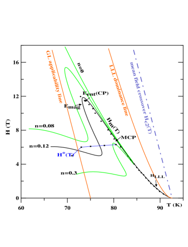
The ”downward shift” of the first order transition line in the plane
It was noted in section III that in a clean system a homogeneous state exists as a metastable overcooled liquid state all the way down to zero temperature (not just below the melting temperature corresponding to , see the line in Fig.12) . This is of importance since interaction with disorder can convert the metastable state into a stable one. Indeed generally a homogeneous state gains more than a crystalline state from pinning, since it can easier adjust itself to the topography of the pinning centers. At large in particular compared to just . As a result in the presence of disorder the transition line shifts to lower fields. The equation for the melting line is
| (306) |
The universal function , plotted in Fig.13 turns out to be non-monotonic. This is an important fact. Since is a monotonic function of , one obtains the transition lines for various in Fig.12 by “sweeping” the Fig.13. A peculiar feature of is that it has a local minimum at and a local maximum at (before crossing zero at . Therefore between these two points there are three solutions to the melting line equation. As a result, starting from the zero field at the transition field reaches a maximum at beyond which the curve sharply turns down (this feature was called “inverse melting” in Avraham et al. (2001)) and at backwards. Then it reaches a minimum and continues as the Bragg glass – vortex glass line roughly parallel to the axis.
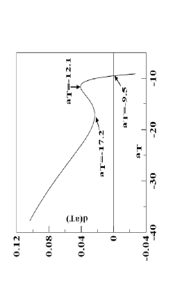
The temperature dependence of the disorder strength , as of any parameter in the GL approach should be derived from a microscopic theory or fitted to experiment. General dependence near is: . The extra factor , not appearing in a phenomenological derivation Blatter et al. (1994), is due to the fact that near order parameter is small and disorder (oxygen deficiencies) locally destroys superconductivity rather than perturbatively modifies the order parameter. The curves in Fig.12 correspond to the disorder strength . The best fit for the low field part of the experimental melting line of the optimally doped YBCO (data taken from Schilling et al. (1996), , ) gives , , (it is consistent with other experiments, for example, Shibata et al. (2002); Deligiannis et al. (2000)). This part is essentially independent of disorder. The upper part of the melting curve is very sensitive to disorder: both the length of the “finger” and its slope depend on . The best fit is This value is of the same order of magnitude as the one obtained phenomenologically using eq.(3.82) in ref. Blatter et al. (1994). We speculate that the low temperature part of the “unified” line corresponds to the solid – vortex glass transition observed in numerous experiments Shibata et al. (2002); Schilling et al. (1996, 1997); Bouquet et al. (2001); Kokkaliaris et al. (2000); Radzyner et al. (2002); Pal et al. (2001, 2002), see data (squares in Fig.12) taken from Shibata et al. (2002). A complicated shape of the “wiggling” line has been recently observed Pal et al. (2001, 2002). Now we turn to a more detailed characteristics of the phase transition.
Discontinuities across the transition and the Kauzmann point. Absence of a second order transition.
Magnetization and specific heat of both solid and liquid can be calculated from the above expressions for free energy. Magnetization of liquid along the melting line is larger than that of solid. The magnetization jump is compared in Li and Rosenstein (2003)a with the SQUID experiments Schilling et al. (1997) in the range (triangles) and of the torque experiments (stars Willemin et al. (1998) and circles Shibata et al. (2002) ). One observes that the results of the torque experiments compare surprisingly well above , but those of Shibata et al. (2002) vanish abruptly below unlike the theory and are inconsistent with the specific heat experiments Schilling et al. (1996); Deligiannis et al. (2000) discussed below. The SQUID data are lower than theoretical (same order of magnitude though). We predict that at lower temperatures (somewhat beyond the range investigated experimentally so far) magnetization reaches its maximum and changes sign at the point (at which magnetization of liquid and solid are equal).
In ref.Li and Rosenstein (2003), entropy jump was calculated using the Clausius – Clapeyron relation and compared with an experimental one deduced from the spike of the specific heat (Schilling et al. (1996), and an indirect measurement from the magnetization jumps (in ref.Shibata et al. (2002)). At high temperatures the theoretical values are a bit lower than the experimental and both seem to approach a constant at . The theoretical entropy jump and the experimental one of Schilling et al. (1996) vanish at (Fig. 12) near . Such points are called Kauzmann points. Below this temperature entropy of the liquid becomes smaller than that of the solid. Note that the equal magnetization point is located at a slightly lower field than the equal entropy point . Experimentally a Kauzmann point was established in BSCCO as a point at which the “inverse melting” appears Avraham et al. (2001). The Kauzmann point observed at a lower temperature in YBCO in ref. Radzyner et al. (2002) is different from since it is a minimum rather than a maximum of magnetic field. It is also located slightly outside the region of applicability of our solution. The point is observed in Pal et al. (2001, 2002) in which the universal line is continuous.
In addition to the spike, the specific heat jump has also been observed along the melting line Schilling et al. (1997, 1996); Deligiannis et al. (2000). Theoretically the jump does not vanish either at or , but is rather flat in a wide temperature range. Our results are larger than experimental jumps of Schilling et al. (1996) (which are also rather insensitive to temperature) by a factor of 1.4 to 2 Li and Rosenstein (2003). In many experimental papers there appears a segment of the second order phase transition continuing the first order melting line beyond a certain point. In Bouquet et al. (2001) it was shown that at that point the specific heat profile shows ”rounding”. We calculated the specific heat profile above the universal first order transition line. It exhibits a ”rounding” feature similar to that displayed by the data of Schilling et al. (1996, 1997, 2002); Bouquet et al. (2001) with no sign of the criticality. The height of the peak is roughly of the size of the specific heat jump. We therefore propose not to interpret this feature as an evidence for a second order transition above the first order line.
Limitations of the perturbative approach
Of course the perturbative approach is limited to small couplings only. In fact, when the correction is compared to the main part of the lattice energy the range become too narrow for practical applications in low temperature superconductors. For high superconductors thermal fluctuations cannot be neglected at higher temperatures since it ”melts” the lattice and even at low temperatures provides thermal depinning. On the conceptual side, it is clear that disorder contributes to destruction of the translational and rotational order. Therefore at certain disorder strength, vortex matter might restore the translation and rotation symmetries, even without help of thermal fluctuations. It is possible to use the perturbation theory in disorder with the liquid state as a starting point in the case of large thermal fluctuations, however it fails to describe the most interesting phenomenon of the vortex glass introduced by Fisher Fisher (1989); Fisher et al. (1991). Therefore one should try to develop non - perturbative methods to describe disorder This is the subject the following sections.
IV.2 The vortex glass
When thermal fluctuations are significant the efficiency of imperfections to pin the vortex matter is generally diminished. This phenomenon is known as ”thermal depinning”. In addition, as we have learned in section III, the vortex lattice becomes softer and eventually melts via first order transition into the vortex liquid. The inter - dependence of pinning, interactions and thermal fluctuations is very complex and one needs an effective nonperturbative method to evaluate the disorder averages. Such a method, using the replica trick was developed initially in the theory of spin glasses. It is more difficult to apply it in a crystalline phase, so we start from a simpler homogeneous phase (the homogeneity might be achieved by both the thermal fluctuations and disorder) and return to the crystalline phase in the following subsection.
IV.2.1 Replica approach to disorder
The replica trick
The replica method is widely used to study disordered electrons in metals and semiconductors, spin glasses and other areas of condensed matter physics and far beyond it Itzykson and Drouffe (1991). It was applied to vortex matter in the elastic medium approximation Nattermann (1990); Bogner et al. (2001); Korshunov (1993); Giamarchi and Le Doussal (1994, 1995a, 1995b, 1996, 1997). In the following we describe the method in some detail.
The main problem in calculation of disorder averages is that one typically has to take the average of non - polynomial functions of the statistical sum eq.(18):
| (307) |
Most interesting physical quantities are calculated by taking derivatives of the free energy which is a logarithm of . Applying a simple mathematical identity to represent the logarithm as a small power, , the average over the free energy is written as:
| (308) |
The quantity can be looked upon as a statistical sum over identical ”replica” fields , :
| (309) |
where is the free energy (in physical units meantime) without disorder. Note that the disorder potential enters in the exponent. The disorder measure, consistent with variance in eq.(273) is a gaussian. Therefore disorder average is a gaussian integral which can be readily performed:
where
| (311) |
After the disorder average different replicas are no longer independent. In LLL limit and units,
| (312) | |||||
This statistical physics model is a type of scalar field theory and the simplest nonperturbative scheme commonly used to treat such a model is gaussian approximation already introduced in IIIB. Its validity and precision can be checked only by calculating corrections.
Correlators and distributions
Correlators averaged over both the thermal fluctuations and disorder can be generated by the usual trick of introducing an external ”source” into statistical sum eq.(307):
| (313) | |||
and taking functional derivatives of the free energy in the presence of sources
| (314) |
The first two thermal correlators are
| (315) | |||
Now the disorder averages of these quantities are made using the replica trick
| (316) | |||
Similar calculation for the two field correlator result in
| (317) |
In disorder physics it is of interest to know the disorder distribution of physical quantities like magnetization (which within LLL is closely related to the correlator, see IIIB). The simplest example is the second moment of the order parameter distribution . This is harder to evaluate due to two thermal averages. One still uses eq.(315) twice:
| (318) | |||
In case of replica symmetry breaking, the formula above shall be written as
| (320) |
Therefor
| (321) | |||||
Disordered LLL theory
Restricting the order parameter to LLL (eq.(112)) by expanding it in quasi - momentum LLL functions eq.(276), one obtains the disordered LLL theory. Let us also rewrite the model in the same units we have used in section III. The resulting Boltzmann factor is
| (322) |
with the disorder term
| (323) | |||||
in which was defined in eq.(142).
IV.2.2 Gaussian approximation
Gaussian energy in homogeneous (amorphous) phase
One can recover the perturbative results of the previous subsection and even generalize them to finite temperatures, by expanding in , however the replica method’s advantage is more profound when nonperturbative effects are involved. We now apply the gaussian approximation, which has been already used in vortex physics in the framework of the elastic medium approach, Korshunov (1993, 1990); Giamarchi and Le Doussal (1994, 1995a, 1995b, 1996, 1997) following its use in polymer and disordered magnets’ physics Mezard (1991). As usual, homogeneous phases are simpler than the crystalline phase considered in the previous subsection, so we start from the case in which both the translational and the symmetries are respected by the variational correlator:
| (324) |
Since the gaussian approximation in the vortex liquid within the GL approach was described in detail in section III, we just have to generalize various expressions to the case of replicas. The gaussian effective free energy is expressed via variational parameter Mezard (1991); Li and Rosenstein (2002a, b, c) which in the present case is a matrix in the replica space. The bubble and the trace log integrals appearing in the free energy are very simple:
| (325) |
where the ”inverse mass” matrix was defined. As a result the gaussian effective free energy density can be written in a form:
| (326) | |||
where we discarded an (ultraviolet divergent) constant and higher order in , and for simplicity, is denoted by .
Minimization equations
It is convenient to introduce a real (not necessarily symmetric) matrix , which is in one - to - one linear correspondence with Hermitian (generally complex) matrix via
| (327) |
Unlike , all the matrix elements of are independent. In terms of this matrix the free energy can be written as
| (328) |
Taking derivative with respect to independent variables gives the saddle point equation for this matrix element:
| (329) | |||
Since the electric charge (or the superconducting phase) symmetry is assumed, we consider only solutions with real . In this case is a symmetric real matrix.
The replica symmetric matrices Ansatz and the Edwards - Anderson order parameter
Experience with very similar models in the theory of disordered magnets indicates that solutions of these minimization equations are most likely to belong to the class of hierarchical matrices, which will be described in the next subsection, We limit ourselves here to most obvious of those, namely to matrices which respect the replica permutation symmetry
| (330) |
for any of permutations If we include also disorder in term, one will find in the low temperature region, replica symmetry is spontaneously breaking as soon as the Edwards -Anderson (EA) order parameter is non zero. However we will limit our discussion to replica symmetric solution (not considering disorder in ) and think that the glass transition appears when the EA order parameter is non zero. This transition line from zero EA to non zero EA obtained in the following is very near to the replica symmetry breaking transition line considering weak disorder in Li et al. (2006b). We also believe that even without disorder in term, the replica symmetry is breaking if we can solve the model non perturbatively.
The most general matrix of the replica symmetric solution has a form
| (331) |
The off diagonal elements are equal to the Edwards - Anderson (EA) order parameter . A nonzero value for this order parameter signals that the annealed and the quenched averages are generally different. Let us calculate starting from the eq.(319). Using the eq.(324) , one obtains in gaussian approximation
| (332) |
where contains also space average.
One can visualize this phase as a phase with locally broken symmetry with various directions of the phase at different locations with zero average but a distribution of non zero value of characteristic width . Distribution of more complicated quantities will be discussed in the last subsection. Here we will refer to this state as glass, although in the subsection E it will be referred to as the ”ergodic pinned liquid” (EPL) distinguished from the ”nonergodic pinned liquid” (NPL) in which, in addition, the ergodicity is broken. Broken ergodicity is related to ”replica symmetry breaking”, however, as we show there, in the present model of the disorder and within gaussian approximation RSB does not occur. If the EA order parameter is zero, disorder doesn’t have a profound effect on the properties of the vortex matter. We refer to this state just as ”liquid”.
The dynamic properties of such phase are generally quite different from those of the non -glassy (zero EA order parameter) phase. In particular it is expected to exhibit infinite conductivity Fisher (1989); Fisher et al. (1991); Dorsey et al. (1992). However if is replica symmetric, pinning does not results in the multitude of time scales. Certain time scale sensitive phenomena like various memory effects Paltiel et al. (2000a, b); Xiao et al. (2002) and the responses to “shaking” Beidenkopf et al. (2005) are expected to be different from the case when breaks the replica permutation symmetry.
We show in the following subsection that within the gaussian approximation and the limited disorder model that we consider (the inhomogeneity only) RSB does not occur. After that is shown, we can consider the remaining problem without using the machinery of hierarchical matrices.
Properties of the replica symmetric matrices
It is easy to work with the RS matrices like in eq.(331). It has two eigenvalues. A replica symmetric eigenvector
| (333) |
where sub leading terms at small , were omitted in the last line, and the rest of the space (replica asymmetric vectors) which is times degenerate. For example
| (334) |
The counting seems strange, but mathematically can be defined and works. Numerous attempts to discredit replica calculations on these grounds were proven baseless. Note that the two eigenvalues differ by order terms only. Projectors on these spaces are
| (340) | |||||
Here is the unit matrix It is easy to invert RS matrices and multiply them using this form. For example
| (341) |
IV.2.3 The glass transition between the two replica symmetric solutions
The unpinned liquid and the “ergodic glass” replica symmetric solutions of the minimization equations
The minimization equation eq.(329) for RS matrices takes a form
| (342) | |||
Expressing it via independent matrices and one obtains:
| (343) | |||
To leading order in (first) the equation is
| (344) |
This means that there exists a RS symmetric solution . In addition there is a non diagonal one. It turns out that there is a third order transition between them.
The second equation,
| (345) |
for the diagonal (”liquid”) solution, is just a cubic equation:
| (346) |
For the non - diagonal solution the first equation eq.(344) gives , which, when plugged into the first equation, gives:
| (347) |
The matrix therefore is
| (348) |
The two solutions coincide when leading to the glass line equation
| (349) |
Free energy and its derivatives. The third order glass line.
Let us now calculate energies of the solutions. Energy of such a RS matrix is given, using eq.(341), by
| (350) | |||
where leading order in small was kept. The RS energy is
| (351) |
which can be further simplified by using eq.(346),
| (352) |
The glass free energy is even simpler:
| (353) |
Since in addition to the energy, the first derivative of the scaled energy, the scaled entropy
| (354) |
and the second derivative, specific heat,
| (355) |
respectively, coincide for both solution on the transition line defined by eq.(349). The third derivatives are different so that the transition is a third order one.
Hessian and the stability domain of a solution
Up to now we have found two homogeneous solutions of the minimization equations. There might be more and the solutions might not be stable, when considered on the wider set of gaussian states. In order to prove that a solution is stable beyond the set of replica symmetric matrices , one has to calculate the second derivative of free energy (so called Hessian) with respect to arbitrary real matrix defined in eq.(327):
| (356) | |||
The Hessian should be considered as a matrix in a space, which itself is a space of matrices, so that Hessian’s index contains two pairs of indices of . We will use a simplified notation for the product of the Kronecker delta functions with more than two indices: . It is not trivial to define what is meant by ”positive definite” when the number of components approaches zero. It turns out that the correct definition consists in finding all the eigenvalues of the Hessian ”super” matrix.
Stability of the liquid solution
For the diagonal solution the Hessian is a very simple operator on the space of real symmetric matrices:
| (357) |
where the operators (the identity in this space) and are defined as
| (358) |
and their coefficients in the liquid phase are:
| (359) |
with being a solution of eq.(346). The corresponding eigenvectors in the space of symmetric matrices are
| (360) |
To find eigenvalues of we apply the Hessian on a vector . The result is (dropping terms vanishing in the limit ):
| (361) | |||||
There two eigenvalues are therefore: and . Since the sufficient condition for stability is:
| (362) |
It is satisfied everywhere below the transition line of eq.(349).
The stability of the glass solution
The analysis of stability of the non - diagonal solution is slightly more complicated. The Hessian for the non - diagonal solution is:
| (363) |
where new operators are
| (364) |
and coefficients are
| (365) |
In the present case, one obtains three different eigenvalues, de Alameida and Thouless (1978); Fischer and Hertz (1991); Dotsenko (2001)
| (366) |
and Note that the eigenvalue of Hessian on the antisymmetric matrices are degenerate with eigenvalue in this case (we will come back later on this eigenvalue). For the solution is unstable due to negative For both eigenvalues are positive and the solution is stable. The line coincides with the third order transition line, hence the non diagonal solution is stable when the diagonal is unstable and vise versa. We conclude that one of the two RS solutions is stable for any value of external parameters (here represented by and ). There still might be a replica asymmetric solution with first order transition to it, but this possibility will be ruled out within the gaussian approximation and in the homogeneous phase without the disorder term in the next subsection. Therefore the transition does not correspond to RSB. Despite this in the phase with nonzero EA order parameter there are Goldstone bosons corresponding to in the replica limit of . The criticality and the zero modes due to disorder (pinning) in this phase might lead to great variety of interesting phenomena both in statics and dynamics.
Generalizations and comparison with experimental irreversibility line
The glass line resembles typical irreversibility lines in both low and high materials, see Fig. 14, where the irreversibility line of is fitted.
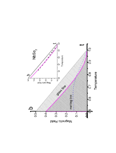
The theory can be generalized to 2D GL model describing thin films or very anisotropic layered superconductors. The glass line is given in 2D
| (367) |
An examples of organic superconductor Shibauchi et al. (1998) was given in Li et al. (2006b). The data of BSCCO Beidenkopf et al. (2005) are compared to the theoretical results on Fig. 15.
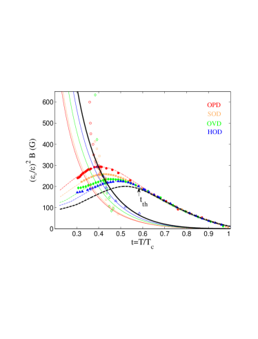
IV.2.4 The disorder distribution moments of the LLL magnetization
As was discussed in III, the magnetization within LLL is proportional to the superfluid density, whose average is
| (368) | |||
The variance of the distribution is determined from the two thermal averages disorder average:
| (369) |
Within gaussian approximation (Wick contractions) the correlators are
| (370) |
Therefore variance of the distribution is given by . This variance determines the width of the magnetization loop. In turn, according to the phenomenological Bean model Tinkham (1996) , the width of the magnetization loop is proportional to the critical current. The distribution of magnetization is not symmetric, as the third moment shows:
| (371) |
It’s calculation is more involved. The third irreducible cumulant is therefore nonzero:
| (372) |
In analogy to ref. Mezard (1991) one can define ”glass susceptibility”
| (373) |
useful in description of the ”glassy” state. Its variance of susceptibility vanishes without RSB:
| (374) |
We return to the replica symmetry breaking after considering the crystalline phase.
IV.3 Gaussian theory of a disordered crystal
IV.3.1 Replica symmetric Ansatz in Abrikosov crystal
In subsection A we used perturbation theory in disorder to assess the basic properties of the vortex crystal. However we learned in the previous subsection that certain properties like the glass related phenomena cannot be captured by perturbation theory and one has to resort to simplest nonperturbative methods available. In the homogeneous phase gaussian approximation in the replica symmetric subspace was developed and we now generalize to a more complicated crystalline case. This is quite analogous to what we did with thermal fluctuations, so the description contains less details.
Replica symmetric shift of the free energy
Within the gaussian approximation the expectation values of the fields as well as their propagators serve as variational parameters. To implement it, it is convenient to shift and ”rotate” the fields according to eq.(143):
| (375) |
where factor was introduced for convenience and are the quasimomentum functions. In principle the shift as well as fields are replica index dependence. However assumption of the unbroken replica symmetry means that
| (376) |
is the only variational shift parameter.
To evaluate gaussian energy we first substitute this into free energy and write quadratic, cubic and quartic parts in fields and . The quadratic terms originating from the interaction and disorder term are listed below. The terms coming from the interaction part are: the term
| (377) | |||
the term , and finally the term . Sum over all four terms is therefore
| (378) |
Similarly the terms sum up to:
| (379) |
while the terms cancel. The disorder term contributes (leading order in , as usual for replica method):
to the part and
| (381) |
to the part. The quadratic part of the free energy therefore is:
| (382) |
There is no linear term and cubic term is not needed since its contraction vanishes. The quartic term will be taken into account later. We will not need cubic terms within the gaussian approximation, while the quartic terms are not affected by the shift of fields. We are ready therefore to write down the gaussian variational energy.
Gaussian energy
Now we describe briefly the contributions to the gaussian energy. The mean field terms (namely containing the shift only with no pairings) are
| (383) |
which using eq.(375) takes a form:
| (384) |
The last term can be omitted since the power of exceeds . Gaussian effective energy in addition to contains the Trlog term and the ”bubble diagrams”. The Trlog term comes from free gaussian part, see section III. The reference ”best gaussian (or quadratic) energy” is defined variationally as a quadratic form
| (385) | |||
and
| (386) |
where are all variational parameters. We assumed no mixing of the and the modes, following the experience in the clean case and the structure of the quadratic part determined in the previous subsection.
In the following we keep sub leading terms in since they contribute to order in energy. The Trlog (divided by volume) is sum of logarithms of all the eigenvalues.
| (387) |
where in the last line integration is over Brillouin zone. One observes that the order terms cancel, while the relevant order is:
| (388) |
The diagrams are of two kinds. Those including one propagator and ones which have two propagators from the part quartic in fields. The propagators are expectation values of pair of fluctuating fields obtained by inverting the replica symmetric matrix like in the previous subsection. For example for the acoustic mode one gets:
| (389) |
The integrals of the propagators over give:
| (390) | |||
and similarly for .
The contraction of the quadratic parts, after the integration and expanded to order results in:
| (391) |
For quartic terms coming from two contractions of the interaction and the disorder part one obtains,
and
| (393) | |||
respectively. Finally we get
| (394) |
IV.3.2 Solution of the gap equations
Gap and shift equations
The gaussian energy is minimized with respect to variational parameters. Differentiating with respect to one gets the ”shift” equation:
| (395) | |||
while differentiating with respect to four variational parameters in the propagator matrix gap equations are obtained
| (396) | |||||
| (397) |
where
Solution by the mode expansion
One can observe that the Ansatz
| (398) |
satisfies the gap equations, leading to simpler set for two unknown functions and three unknown parameters satisfying eqs.(395),(396),(397) and:
| (399) | |||||
The equation can be solved by using mode expansion:
| (400) |
As in IIIC, The integer determines the distance of a points on reciprocal lattice from the origin. and . One estimates that therefore the coefficients decrease exponentially with . Note that for some integers, for example , . Retaining only first modes will be called ”the mode approximation”.
| (401) | |||||
The expression deviates significantly from the perturbative one, especially at low temperatures and when the 2D case is considered.
Generalizations and comparison to experiments
As we noted already in 2D disorder leads, at least perturbatively, to more profound restructuring of the vortex lattice than in 3D. In fact perturbation theory becomes invalid. The gaussian methods described above remove the difficulty and allow calculation of the order - disorder lime. In this case one does not encounters the ”wiggle” but rather a smooth decrease of the order - disorder field, when temperature becomes lower. In Fig. 15 the ODO line of strongly anisotropic high superconductor is shown.
One generally observes that there is always off diagonal component in the correlator of the ”optical” phonon field . However the off diagonal Edwards - Anderson parameter part for a more important low energy excitation ”acoustic” branch appears only below a line quite similar to the glass line in the homogeneous phase.
IV.4 Replica symmetry breaking
When thermal fluctuations are significant the efficiency of imperfections to pin the vortex matter is generally diminished. This phenomenon is known as ”thermal depinning”. In addition, as we have learned in section III, the vortex lattice becomes softer and eventually melts via first order transition into the vortex liquid. The inter - dependence of pinning, interactions and thermal fluctuations is very complex and one needs an effective nonperturbative method to evaluate the disorder averages. Such a method, using the replica trick was developed initially in the theory of spin glasses. It is more difficult to apply it in a crystalline phase, so we start from a simpler homogeneous phase (the homogeneity might be achieved by both the thermal fluctuations and disorder) and return to the crystalline phase in the following subsection.
IV.4.1 Hierarchical matrices and absence of RSB for the disorder in gaussian approximation
The hierarchical matrices and their Parisi’s parametrization
Experience with very similar models in the theory of disordered magnets indicates that solutions of these minimization equations are most likely to belong to the class of hierarchical matrices, which are comprehensively described, for example in Fischer and Hertz (1991); Dotsenko (2001); Mezard (1991), We limit ourselves here to operational knowledge of working with such matrices contained in Appendix of ref. Mezard (1991) and collect several rules of using the Parisi’s representation in Appendix B. General hierarchical matrices are parametrized using the diagonal elements and the Parisi’s (monotonically increasing) function specifying the off diagonal elements with Parisi (1980). Physically different represent time scales in the glass phase. In particular the Edwards - Anderson (EA) order parameter is .
A nonzero value for this order parameter signals that the annealed and the quenched averages are different. The dynamic properties of such phase are generally quite different from those of the non glassy phase. In particular it is expected to exhibit infinite conductivity Fisher (1989); Fisher et al. (1991); Dorsey et al. (1992). We will refer to this phase as the ”ergodic pinned liquid” (EPL) distinguished from the ”nonergodic pinned liquid” (NPL) in which, in addition, the ergodicity is broken. Broken ergodicity is related to ”replica symmetry breaking” discussed below, however, as we show shortly, in the present model of the disorder and within gaussian approximation RSB does not occur.
In terms of Parisi parameter and the matrix equation eq.(329) takes a form:
| (402) |
| (403) |
Dynamically (see next section), if is a constant, pinning does not results in the multitude of time scales. Certain time scale sensitive phenomena like various memory effects Paltiel et al. (2000a, b); Xiao et al. (2002) and the responses to “shaking” Beidenkopf et al. (2005) are expected to be different from the case when takes multiple values. If takes a finite different number of values, we call step RSB. On the other hand, if is continuous, the continuous replica symmetry breaking (RSB) occurs. We show below that within the gaussian approximation and the limited disorder model that we consider (the inhomogeneity only) RSB does not occur. After that is shown, we can consider the remaining problem without using the machinery of hierarchical matrices.
Absence of replica symmetry breaking
In order to show that is a constant, it is convenient to rewrite the second equation via the matrix the matrix inverse to :
| (404) |
Differentiating this equation with respect to one obtains;
| (405) |
where we used a set of standard notations in the spin glass theory: Mezard (1991)
| (406) | |||||
If one is interested in a continuous monotonic part the only solution of eq.(404) is
| (407) |
Differentiating this again and dropping the nonzero derivative again, one further gets a contradiction: . This proves that there are no such monotonically increasing continuous segments. One can therefore generally have either the replica symmetric solutions, namely or look for a several step - like RSB solutions Fischer and Hertz (1991); Dotsenko (2001). One can show that the constant solution is stable. Therefore, if a step - like RSB solution exists, it might be only an additional local minimum. We explicitly looked for a one step solution and found that there is none.
V Summary and perspective
In this section we summarize and provide references to original papers, point out further applications and generalizations of results presented here. The bibliography of works on the GL theory of the vortex matter is so extensive that there, no doubt, many important papers and even directions are missed in this brief outline. Some of them however can be found in books Kopnin (2001); Larkin and Varlamov (2005); Saint-James et al. (1969); Ketterson and Song (1999); Tinkham (1996) and reviews Blatter et al. (1994); Nattermann and Scheidl (2000); Brandt (1995); Giamarchi and Bhattacharya (2002).
V.1 GL equations.
Microscopic derivations of the GL equations
Phenomenological Ginzburg - Landau equations Ginzburg and Landau (1950) preceded a microscopic theory of superconductivity. Soon after the BCS theory appeared Gorkov and others derived from it the GL equations. Derivations and the relations of the GL parameters to the microscopic parameters in the BCS theory are reviewed in the book by Larkin and Varlamov Larkin and Varlamov (2005) (where extensive bibliography can be found). The dynamical versions of the theory were derived using several methods and the parameter in the time dependent GL equation related no the normal state conductivity Larkin and Varlamov (2005). Most of the methods described here can be generalized to the case, when the non - dissipative imaginary part of is also present. In particular this leads to the Hall current Ullah and Dorsey (1990, 1991); Troy and Dorsey (1993) and was used to explain the ”Hall anomaly” in both low and high superconductors.
The disorder was introduced phenomenologically in statics in Larkin (1970). Other coefficients of the GL free energy may also have random components Blatter et al. (1994). How these new random variables influence the LLL model was discussed in Li et al. (2006b).
Anisotropy
High cuprates are layered superconductors which can be better described by the Lawrence - Doniach (LD) model Lawrence and Doniach (1971) than the 3D GL model discussed in the present review. The LD model, is a version of the GL model with a discretized coordinate. However in many cases one can use two simpler limiting cases. If anisotropy is not very large one can use anisotropic 3D GL, eq.(5). The requirement, that the GL can be effectively used, therefore limits us to optimally doped and similar materials for which the anisotropy parameter is not very large: . Effects of layered structure are dominant in or based compounds () and noticeable for cuprates with anisotropy of order like or . Anisotropy effectively reduces dimensionality leading to stronger thermal fluctuations according to eq,(19). Very anisotropic layered superconductors can be described by 2D GL model
| (408) |
which can be approached by the methods presented here. For LD model analytical methods become significantly more complicated. The gaussian approximation study of thermal fluctuations was however performed Ikeda (1995); Larkin and Varlamov (2005) and used to explained the, so called crossing point of the magnetization curves, as well as crossover between the to the behaviorBaraduc et al. (1994); Salem-Sugui and Dasilva (1994); Junod et al. (1998); Rosenstein et al. (2001); Huh and Finnemore (2002); Tešanović et al. (1992); Lin and Rosenstein (2005) In many simulations this model rather than GL was adopted Ryu et al. (1996); Wilkin and Jensen (1997). The GL model can be extended also in direction of introducing anisotropy in the plane, like the four - fold symmetric anisotropy leading to transition from the rhombic lattice to the square lattice Chang et al. (1998a, b); Klironomos and Dorsey (2003); Park and Huse (1998); Rosenstein and Knigavko (1999) observed in many high and low type II superconductors alike Eskildsen et al. (2001); Li et al. (2006a) .
Dynamics
Dynamics of vortex matter can be described by a time dependent generalization of the GL equations Larkin and Varlamov (2005). The bifurcation method presented here can be extended to moving vortex lattice Thompson and Hu (1971); Li et al. (2004b). The extension is nontrivial since the linear operator appearing in the equations is non Hermitian.
V.2 Theory of thermal fluctuations in GL model
Here we briefly list various alternative approaches to those described in the present review. It is important to mention an unorthodox opinion concerning the very nature of the crystalline state and melting transition. Although a great variety of recent experiments indicate that the transition is first order (for alternative interpretation see Nikulov et al. (1995a); Nikulov (1995b)), some authors doubt the existence of a stable solid phase Moore (1989, 1992); Kienappel and Moore (1997) and therefore of the transition all together.
Functional renormalization group for the LLL theory
While applying the renormalization group (RG) on the one loop level, Brézin, Nelson and Thiaville Brézin et al. (1985) found no fixed points of the (functional) RG equations and thus concluded that the transition to the solid phase, if it exists, is not continuous. The RG method therefore cannot provide a quantitative theory of the melting transition. It is widely believed however that the finite temperature transition exists and is first order (see however Newman and Moore (1996), who found another solution of functional RG equations).
Large number of components limit
The GL theory can be generalized (in several different ways) to an component order parameter field. The large limit of this theory can be computed in a way similar to that in the component scalar models widely used in theory of critical phenomena Itzykson and Drouffe (1991). The most straightforward generalization has been studied in Affleck and Brézin (1985) in the homogeneous phase leading to a conclusion that there is no instability of this state in the 3D GL. However since there are other ways to extend the theory to the component case, it was shown in Moore et al. (1998) that the state in which only one component has a nonzero expectation value (similar to the one component Abrikosov lattice) is not the ground state of the most straightforward generalization. Subsequently it was found Lopatin and Kotliar (1999); Li et al. (2004a) that there exists a generalization for which this is in fact the case .
Diagrams resummation
In many body theories one can resum various types of diagrams. In fact one can consider Hartree-Fock, and even one loop RG as kinds of the diagrams resummation. Moore and Yeo Yeo and Moore (1996a, b, 2001) and more recently Yeo with his coworkers Yeo et al. (2006); Park and Yeo (2008) followed a strategy used in strongly coupled electron systems to resum all the parquet diagrams. The thermal fluctuation in GL model had been studied using various analytic methods Koshelev (1994), but in the vortex liquid region near the melting point,or overcooled liquid, non-perturbative method must be used, for example, Borel-Pade resummation method to obtain density density correlation was carried out in ref.Hu et al. (1994).
Numerical simulations
The LLL GL model was studied numerically in both 3D Sasik and Stroud (1995) and 2D Tešanović and Xing (1991); O’Neill and Moore (1993); Kato and Nagaosa (1993); Li and Nattermann (2003). The melting was found to be first order. The results serve as an important check on the analytic theory described in this review. In many simulations the XY model is employed Ryu et al. (1996); Hu et al. (1997); Wilkin and Jensen (1997). It is believed that results are closely related to that of the Ginzburg - Landau model. The methods allows consideration of disorder and dynamics Nonomura and Hu (2001); Olsson and Teitel (2001); Chen and Hu (2003); Olsson (2007) and fluctuations of the magnetic field Nguyen and Sudbø (1998); Sudbø and Nguyen (1999).
Density functional
The density functional theory is a general method to tackle a strongly coupled system. The method crucially depends on the choice of the functional. It was applied to the GL model by Herbut and Tešanović Herbut and Tešanović (1994) and was employed in Menon and Dasgupta (1994); Menon et al. (1999); Menon (2002) to study the melting and in Hu et al. (2005) to the layered systems.
Vortex matter theory
Elastic moduli were first calculated from the GL model by Brandt Brandt (1977a, b, 1986) by considering an infinitesimal shift of zeroes of the order parameter. He found that the compression and the shear moduli are dispersive. This feature is important in phenomenological applications like the Lindemann criterion for both the melting and the order - disorder lines (considered different) Houghton et al. (1989); Ertas and Nelson (1996); Kierfeld and Vinokur (2000); Mikitik and Brandt (2001, 2003), as well to estimates of the critical current and the collective pinning theory (see reviews Brandt (1995); Blatter et al. (1994) and references therein). The dispersion however is ignored in most advanced applications of the elasticity theory to staticsGiamarchi and Le Doussal (1994, 1995a, 1995b, 1996, 1997); Nattermann and Scheidl (2000) or dynamicsGiamarchi and Le Doussal (1996); Chauve et al. (2000); Giamarchi and Le Doussal (1998); Giamarchi and Bhattacharya (2002). Recently a phase diagram of strongly type II superconductors was discussed using a modified elasticity theory taking into account dislocations of the vortex lattice Dietel and Kleinert (2006, 2007, 2009)
Tešanović and coworkers noted Tešanović et al. (1992); Tešanović and Andreev (1994) a remarkable fact that most of the fluctuations effects are just due to condensation energy. The lateral correlations part are just around 2% and therefore can be neglected. The theory explains an approximate intersection of the magnetization curves and is used to analyze data Zhou et al. (1993); Pierson et al. (1995, 1996); Pierson and Walls (1998a); Pierson et al. (1998b).
Beyond LLL
To quantitatively describe vortex matter higher Landau levels (HLL) corrections are sometimes required. For example in optimally doped superconductor one can establish the LLL scaling for fields above and temperature above (see, for example, Sok et al. (1995)). A glance at the data however shows that above the scaling is generally unconvincing: the LLL magnetization is much larger that the experimental one above . Naively, on the solid side, when the distance from the mean field transition line is smaller than the inter - Landau level gap, one expects that the higher Landau modes can be neglected. More careful examination of the mean field solution presented in subsection IIB reveals that a weaker condition should be used for a validity test of the LLL approximation. However the fluctuation corrections involving HLL in strongly fluctuating superconductors might be important. Ikeda and collaborators calculated the fluctuation spectrum in solid including HLL Ikeda et al. (1990); Ikeda (1995). In the vortex liquid the HLL contribution has been studied by Lawrie Lawrie (1994) in the framework of the gaussian (Hartree - Fock) approximation. He found the region of validity of LLL approximation. The leading (gaussian) contribution of HLL was combined with more refined treatment of the LLL modes recently resulting in reasonably good agreement with experimental data Li and Rosenstein (2003).
Fluctuations of magnetic field and the dual theory approach
Although it was understood that fluctuations of the magnetic field in strongly type II superconductors are strongly suppressed Halperin et al. (1974); Lobb (1987), they still play an important role when is not large and magnetic field away from (the situation mostly not covered in the present review). The main methods are the numerical simulations Dasgupta and Halperin (1981); Sudbø and Nguyen (1999); Olsson and Teitel (2003) and the dual theory approach Tešanović (1999); Kovner and Rosenstein (1992); Kovner et al. (1993), which was very efficient in describing the Kosterlitz - Thouless transition in superconducting thin film and layered materials Oganesyan et al. (2006). Vortex lines and loops are interpreted as a signal of ”inverted ” or the ”magnetic flux” symmetry. The symmetry is spontaneously broken in the normal phase (with photon as a Goldstone boson), while restored in the superconductor. Vortices are the worldlines of the flux symmetry charges.
V.3 The effects of quenched disorder
Vortex glass in the frustrated XY model
The original idea of the vortex glass and the continuous glass transition exhibiting the glass scaling of conductivity diverging in the glass phase appeared early in the framework of the so called frustrated model (the gauge glass) Fisher (1989); Fisher et al. (1991); Nattermann and Scheidl (2000). In this approach one fixes the amplitude of the order parameter retaining the magnetic field with random component added to the vector potential. It was studied by the RG and variational methods and has been extensively simulated numerically Olsson and Teitel (2001); Olsson (2007); Nonomura and Hu (2001); Chen and Hu (2003); Kawamura (2003); Chen (2008).In analogy to the theory of spin glass the replica symmetry is broken when crossing the GT line. The model ran into several problems (see Giamarchi and Bhattacharya in ref.Giamarchi and Bhattacharya (2002) for a review): for finite penetration depth it has no transition Bokil and Young (1995) and there was a difficulty to explain sharp Bragg peaks observed in experiment at low fields.
Disordered elastic manifolds. Bragg glass and replica symmetry breaking
To address the last problem another simplified model had been proven to be more convenient: the elastic medium approach to a collection of interacting line-like objects subject to both the pinning potential and the thermal bath Langevin force Reichhardt et al. (1996, 2000); van Otterlo et al. (1998); Olson et al. (2001); Cha and Fertig (1994a, b); Faleski et al. (1996); Fangohr et al. (2001, 2003); Dodgson et al. (2000). The resulting theory was treated again using the gaussian approximation Korshunov (1993); Giamarchi and Le Doussal (1994, 1995a, 1995b, 1996, 1997) and RG Nattermann (1990); Bogner et al. (2001); Nattermann and Scheidl (2000). The result was that in there is a transition to a glassy phase in which the replica symmetry is broken following the “hierarchical pattern” (in the breaking is “one step”). The problem of the very fast destruction of the vortex lattice by disorder was solved with the vortex matter being in the replica symmetry broken (RSB) phase and it was termed “Bragg glass”Giamarchi and Le Doussal (1994, 1995a, 1995b, 1996, 1997). A closely related approach was developed very recently for both 3D and layered superconductors in which effects of dislocations were incorporated Dietel and Kleinert (2006, 2007, 2009).
Density functional for a disordered systems, supersymmetry
Generalized replicated density functional theory Menon (2002) was also applied resulting in one step RSB solution.Although the above approximations to the disordered GL theory are very useful in more “fluctuating” superconductors like , a problem arises with their application to at temperature close (where most of the experiments mentioned above are done): vortices are far from being line-like and even their cores significantly overlap. As a consequence the behavior of the dense vortex matter is expected to be different from that of a system of line - like vortices and of the model although the elastic medium approximation might still be meaningful Brandt (1995).
One should note the work by Tešanović and Herbut Tešanović and Herbut (1994) on columnar defects in layered materials, which utilizes supersymmetry, as an alternative to replica or dynamics, to incorporate disorder non - perturbatively.
Dynamical approach to disorder in the Ginzburg - Landau model
The statics and the linear response within disordered GL model has been discussed in numerous theoretical, numerical and experimental works. The glass line was first determined, to our knowledge, using the Martin - Siggia - Rose dynamical approach in gaussian approximation Dorsey et al. (1992) and was claimed to be obtained using resummation of diagram in Kubo formula in Ikeda et al. (1990). The glass transition line for the disorder was obtained using the replica formalism (within similar gaussian approximation) by Lopatin Lopatin (2000) and the result is identical to presented in the present review. He also extended the discussion beyond the gaussian approximation employing the Cornwall - Jackiw - Tomboulis variational method described. This was generalized to other types of disorder (the mean free path disorder) in ref. Li et al. (2006b). The common wisdom is that the ”replica” symmetry is generally broken in the glass (either via ”steps” or via ”hierarchical” continuous process) as in most of the spin glasses theories Fischer and Hertz (1991); Dotsenko (2001). The divergence of conductivity on the glass line was obtained in Rosenstein and Zhuravlev (2007) (it was assumed in ref. Dorsey et al. (1992) and linked phenomenologically to the general scaling theory of the vortex glass proposed in ref. Fisher (1989); Fisher et al. (1991)). Results are consistent with the replica ones presented in the present review). In this work I-V curves and critical current were derived in (improved) gaussian approximation and several physical questions related to the peak effect addressed.
Numerical simulation of the disordered Ginzburg - Landau model
The theory can be generalized to the 2D case appropriate for description of thin films or strongly layered superconductors and compared to experiments. The comparison for organic superconductor type Bel et al. (2007) and Beidenkopf et al. (2005) of the static glass line is quite satisfactory. There exist, to our knowledge, just two Monte Carlo simulations of the disordered GL model Li and Nattermann (2003); Kienappel and Moore (1997), both in 2D, in which no clear irreversibility line was found. However the frustrated XY model was recently extensively simulated Olsson and Teitel (2001); Nonomura and Hu (2001); Chen and Hu (2003); Olsson and Teitel (2003); Kawamura (2003); Olsson (2007); Chen (2008) including the glass transition line and I-V curves It shares many common features with the GL model although disorder is introduced in a different way, so that it is difficult to compare the dependence of pinning. The I-V curves and the glass line resemble the Ginzburg - Landau results.
Finite electric fields
Finite electric fields (namely transport beyond linear response) were also considered analytically in Blum and Moore (1997) and our result in the clean limit agrees with their’s. The elastic medium and the vortex dynamics within the London approximation were discussed beyond linear response in numerous analytic and numerical works. Although qualitatively the glass lines obtained here resemble the ones in phenomenological approaches based on comparison of disorder strength with thermal fluctuations and interaction Mikitik and Brandt (2001, 2003); Ertas and Nelson (1996); Kierfeld and Vinokur (2000); Radzyner et al. (2002), detailed form is different.
V.4 Other fields of physics
There are several physical systems in which the methods described here, in a slightly modified form, can be applied and indeed appeared under different names. One area is the superfluidity and the BEC condensate physics (ref.Pethick and Smith (2008) and references therein).Magnetic field is analogous to the rotation of the superfluid. One can observe lattice of vortices with properties somewhat reminiscent of those of the Abrikosov vortices Madison et al. (2000); Abo-Shaeer et al. (2001); Engels et al. (2002); Cooper et al. (2001); Sinova et al. (2001); Baym (2003); Sonin (2005); Wu et al. (2007). Another closely relate field is the physics of the 2D electron gas in strong magnetic field Monarkha and Kono (2004). In some cases the problem can be formulated in a way similar to the present case with Wigner crystal analogous to the Abrikosov liquid (time playing the role of the direction of the fluxon), while quenched disorder appears in a way similar to the columnar defects in the vortex physics. Some aspects of the physics of the liquid crystal also can be formulated in a form similar to the GL equations in magnetic field.
V.5 Acknowledgments
We are grateful to many people, who either actively collaborated with us or discussed various issues related to vortex physics. Collaborators, colleagues and students include B. Ya. Shapiro, V. Zhuravlev, V. Vinokur, P.J. Lin, T.J. Yang, I. Shapiro, G. Bel, Z.G. Wu, B. Tinh, B. Feng, Z.S. Ma, E. Zeldov, E.H. Brandt, R. Lortz, Y. Yeshurun, P. Lipavsky, and A. Shaulov. We are indebted to T. Maniv, G. Menon, A.T. Dorsey, C. Reichhardt, A.E. Koshelev, S. Teitel. P. Olsson, X. Hu, T. Nattermann, T. Giamarchi, G. Blatter, Z. Tešanović, R. Mintz, and B. Horowitz for discussions, M.K. Wu, E. Andrei, C.C. Chi, P.H. Kes, E.M. Forgan, J. Juang, J.Y. Lib, J.J. Lib, M.R. Eskildsen, H.H. Wen, T. Nishizaki, A. Grover, N. Kokubo, S. Salem-Sugui, K. Hirata, C. Villard, H. Beidenkopf, J. Kolacek, C. J. van der Beek, and M. Konczykowski. for discussions and sending experimental results, sometimes prior to publications. Work supported by NSC of R.O.C. grant, NSC#952112M009048 and MOE ATU program, and National Science foundation of China (#10774005). D.L is grateful to National Chiao Tung University, while B. R. is grateful to NCTS and University Center of Samaria for hospitality during sabbatical leave.
VI Appendices
VI.1 Integrals of products of the quasimomentum eigenfunctions
In this appendix a method to calculate space averages of products of the quasi - momentum eigenfunctions in both static and the dynamic cases.
VI.1.1 Rhombic lattice quasimomentum functions
Let us specialize to a rhombic lattice with following bases of the direct and the reciprocal lattices (see Fig. 3 for definition of the angle and the lattice spacing , subject to the flux quantization relation, eq.(63)):
| (409) | |||||
We use here the ”LLL” unit of magnetic length.
We start with static LLL functions for an arbitrary rhombic lattice:
| (410) | |||||
To include higher LL corrections, it is convenient to use rising and lowering operators introduced in eq.(90) to work with the HLL functions, . The following formula will be frequently used. If is an LLL function, then
| (411) |
VI.1.2 The basic Fourier transform formulas
Product of two functions
It can be verified by direct calculation of gaussian integrals that
| (412) |
with decomposition of arbitrary momentum into its ”rational part” ,which belongs to the Brillouin zone and an ”integer part” , belonging to the reciprocal lattice
| (413) |
Its inverse Fourier transform,
| (414) |
where , can be generalized into
| (415) | |||
with . This in turn provides a very useful product representation:
| (416) | |||
The four - point vertex function
The relation above used twice gives the following expression for the four point vertex:in the quasi - momentum representation:
| (417) | |||
The delta function implies that
| (418) |
As we have only three possible integer values for each coordinate:
| (419) | |||||
which require . Thus
and the product takes a form:
| (421) | |||
where if The last exponent in function can be also rearranged as
| (422) | |||
Using
where is the volume of the unit cell and in our units is equal to , one obtains the Poisson resummation relation,
Using Poisson resummation, one rewrites the sum as
| (423) | |||||
VI.1.3 Calculation of the functions and their small momentum expansion
One often encounters the following space averages:
| (424) |
and Using formulas of the previous subsection, one can write
| (425) | |||
Therefore
| (426) |
and
| (427) |
Similarly can be obtained. for , we have
| (428) |
The above formula is valid for any lattice structure.
Small momentum expansion of the function for the general rhombic lattice
Consider the sum
| (429) |
for any integers . Due to reflection symmetry
| (430) |
for integers, and odd integer. For small :
Similarly for the function can be expanded for small
| (432) |
so that
Small momentum expansion of the function for hexagonal lattice
When the symmetry is higher, the expressions simplify. Using the six - fold symmetry of the hexagonal lattice,
| (434) |
the sum eq.(429) transforms into
| (435) |
Thus if . Using one obtains several relations of different sums to simplify expansion of
| (436) |
Similarly
| (437) |
and its phase has an expansion
| (438) |
In terms of it is an analytic function:
| (439) |
Self duality relation
If the lattice is self-dual, one can prove
| (440) |
Thus
| (441) |
Using the expansion for one can obtain the supersoft acoustic phone spectrum:
| (442) |
The small momentum expansion of the vertex function
For momentum, are not too big to have Umklapp process
| (443) |
where In this case, we define and which has small momentum expansion:
| (444) |
Another useful identity
Any sixfold () symmetric function (namely a function satisfying where is related by a rotation) obeys:
| (445) |
This identity can be proved by using the fact is a analytic function of and is a periodic function of reciprocal lattice vectors, i.g.
| (446) |
the function is unchanged. The only solution for a analytic function with this property is a constant.
| (447) |
The constant can be determined by setting .
VI.2 Parisi algebra for hierarchial matrices
In this appendix we collect without derivation the formulas used in calculation of disorder properties. Derivation can be found in ref. Mezard (1991). Inverse matrix has the following Parisi parameters:
| (448) | |||||
Square of matrix can be treated similarly:
| (449) | |||||
References
- Abo-Shaeer et al. (2001) Abo-Shaeer, J. R., C. Raman, J. M. Vogels, and W. Ketterele, 2001, Science 292, 476.
- Abrikosov (1957) Abrikosov, A. A., 1957, Zh. Eksp. Teor. Fiz. 32, 1442.
- Adesso et al. (2006) Adesso, M. G., D. Uglietti, R. Flükiger, M. Polichetti, and S. Pace, 2006, Phys. Rev. B 73, 092513.
- Affleck and Brézin (1985) Affleck, I.,and E. Brézin, 1985, Nucl. Phys. B 257, 451.
- Avraham et al. (2001) Avraham, N., B. Khaykovich, Y. Myasoedov, M. Rappaport, H. Shtrikman, D. E. Feldman, T. Tamegai, P. H. Kes, M. Li, M. Konczykowski, K. van der Beek, and E. Zeldov, 2001, Nature (London) 411, 451.
- Baker (1990) Baker, G. A., 1990, Quantitative theory of critical phenomena (Academic Press, Boston ).
- Baraduc et al. (1994) Baraduc, C., E. Janod, C. Ayache, and J. Y. Henry, 1994, Physica C 235, 1555.
- Baym (2003) Baym, G., 2003, Phys. Rev. Lett. 91, 110402.
- Bel et al. (2007) Bel, G., D. Li, B. Rosenstein, V. Vinokur, and V. Zhuravlev, 2007, Physica C 460-462, 1213.
- Bellet et al. (1996a) Bellet, B., P. Garcia, and A. Neveu, 1996a, Int. J. Mod. Phys. A 11, 5587.
- Bellet et al. (1996b) Bellet, B., P. Garcia, and A. Neveu, 1996b, Int. J. Mod. Phys. A 11, 5607.
- Bender et al. (1994) Bender, C. M., A. Duncan, and H.F. Jones, 1994, Phys. Rev. D 49, 4219.
- Beidenkopf et al. (2005) Beidenkopf, H., N. Avraham, Y. Myasoedov, H. Shtrikman, E. Zeldov, B. Rosenstein, E. H. Brandt, and T. Tamegai, 2005, Phys. Rev. Lett. 95, 257004.
- Beidenkopf et al. (2007) Beidenkopf, H., T. Verdene, Y. Myasoedov, H. Shtrikman, E. Zeldov, B. Rosenstein, D. Li, and T. Tamegai, 2007, Phys. Rev. Lett. 98, 167004.
- Blatter et al. (1994) Blatter, G., M. V. Feigel’man, V. B. Geshkenbein, A. I. Larkin, and V. M. Vinokur, 1994, Rev. Mod. Phys. 66, 1125.
- Blum and Moore (1997) Blum, T., and M. A. Moore, 1997, Phys. Rev. B 56, 372.
- Bogner et al. (2001) Bogner, S., T. Emig, and T. Nattermann, 2001, Phys. Rev. B 63, 174501.
- Bokil and Young (1995) Bokil, H. S., and A. P. Young, 1995, Phys. Rev. Lett. 74, 3021.
- Bouquet et al. (2001) Bouquet, F., C. Marcenat, E. Steep, R. Calemczuk, W. K. Kwok, U. Welp, G. W. Crabtree, R. A. Fisher, N. E. Phillips, and A. Schilling, 2001, Nature (London) 411, 448.
- Brandt (1977a) Brandt, E. H., 1977a, J. Low Temp.Phys. 26, 709.
- Brandt (1977b) Brandt, E. H., 1977b, J. Low Temp.Phys. 26, 735.
- Brandt (1986) Brandt, E. H., 1986, Phys. Rev. B 34, 6514.
- Brandt (1995) Brandt, E. H., 1995, Rep. Prog. Phys. 58, 1465.
- Brézin et al. (1985) Brézin, E., D.R. Nelson, and A. Thiaville, 1985, Phys. Rev. B 31, 7124.
- Brézin et al. (1990) Brézin, E., A. Fujita,and S. Hikami, 1990, Phys. Rev. Lett. 65, 1949.
- Cha and Fertig (1994a) Cha, M.-C., and H. A. Fertig, 1994a, Phys. Rev. Lett. 73, 870.
- Cha and Fertig (1994b) Cha, M.-C., and H. A. Fertig, 1994b, Phys. Rev. B 50, 14368.
- Chang et al. (1998a) Chang, D., C.-Y. Mou, B. Rosenstein, and C. L. Wu, 1998a, Phys. Rev. Lett. 80, 145.
- Chang et al. (1998b) Chang, D., C.-Y. Mou, B. Rosenstein, and C. L. Wu, 1998b, Phys. Rev. B 57, 7955.
- Chauve et al. (2000) Chauve, P., T. Giamarchi, and P. Le Doussal, 2000, Phys. Rev. B 62, 6241.
- Chen and Hu (2003) Chen, Q. H., and X. Hu, 2003, Phys. Rev. Lett. 90, 117005.
- Chen (2008) Chen, Q. H., 2008, Phys. Rev. B 78, 104501.
- Compagner (1974) Compagner, A., 1974, Physica 72, 115.
- Cooper et al. (2001) Cooper, N. R., N. K. Wilkin, and J. M. F. Gunn, 2001, Phys. Rev. Lett. 87, 120405.
- Cornwall et al. (1974) Cornwall, J. M., R. Jackiw, and E. Tomboulis, 1974, Phys. Rev. D 10, 2428.
- Dasgupta and Halperin (1981) Dasgupta, C., and B. I. Halperin, 1981, Phys. Rev. Lett. 47, 1556.
- David (1981) David, F., 1981, Com. Math. Phys. 81, 149.
- de Alameida and Thouless (1978) de Alameida, J. R. L., and D. J. Thouless, 1978, J. Phys. A 11, 983.
- Deligiannis et al. (2000) Deligiannis, K., M. Charalambous, J. Chaussy, R. Liang, D. Bonn, and W. N. Hardy, 2000, Physica C 341, 1329.
- Dietel and Kleinert (2006) Dietel, J.,and H. Kleinert, 2006, Phys. Rev. B 74, 024515.
- Dietel and Kleinert (2007) Dietel, J.,and H. Kleinert, 2007, Phys. Rev. B 75, 144513.
- Dietel and Kleinert (2009) Dietel, J.,and H. Kleinert, 2009, Phys. Rev. B 79, 014512.
- Divakar et al. (2004) Divakar, U., A. J. Drew, S. L. Lee, R. Gilardi, J. Mesot, F. Y. Ogrin, D. Charalambous, E. M. Forgan, G. I. Menon, N. Momono, M. Oda, C. D. Dewhurst, and C. Baines, 2004, Phys. Rev. Lett. 92, 237004.
- Dodgson et al. (2000) Dodgson, M. J. W., A. E. Koshelev, V. B. Geshkenbein, and G. Blatter, 2000, Phys. Rev. Lett. 84, 2698.
- Dorsey et al. (1992) Dorsey, A. T., M. Huang, and M. P. A. Fisher, 1992, Phys. Rev. B 45, 523.
- Dotsenko (2001) Dotsenko, V., 2001, An Introduction to the Theory of Spin Glasses and Neural Networks (Cambridge University Press,New York ).
- Duncan and Jones (1993) Duncan, A., and H.F. Jones, 1993, Phys. Rev. D 47, 2560.
- Eilenberger (1967) Eilenberger,G., 1967, Phys. Rev. 164, 628.
- Engels et al. (2002) Engels, P., I. Coddington, P. C. Haljian, and E. A. Cornell, 2002, Phys. Rev. Lett. 89, 100403.
- Ertas and Nelson (1996) Ertas, D., and D. R. Nelson, 1996, Physica C 272, 79.
- Eskildsen et al. (2001) Eskildsen, M. R., A. B. Abrahamsen, V. G. Kogan, P. L. Gammel, K. Mortensen, N. H. Andersen, and P. C. Canfield, 2001, Phys. Rev. Lett. 86, 5148.
- Faleski et al. (1996) Faleski, M. C., M. C. Marchetti, and A. A. Middleton, 1996, Phys. Rev. B 54, 12427.
- Fangohr et al. (2001) Fangohr, H., and S. J. Cox, 2001, Phys. Rev. B 64, 064505.
- Fangohr et al. (2003) Fangohr, H., A. E. Koshelev, and M. J. W. Dodgson, 2003, Phys. Rev. B 67, 174508.
- Feng et al. (2009) Feng, B., Z. Wu, and D. Li, 2009, Int. Mod. Phys. B 23, 661.
- Fischer and Hertz (1991) Fischer, K. H., and J. A. Hertz, 1991, Spin glasses (Cambridge University Press,New York ).
- Fisher (1989) Fisher, M. P. A., 1989, Phys. Rev. Lett. 62, 1415.
- Fisher et al. (1991) Fisher, D. S., M. P. A. Fisher, and D. A. Huse, 1991, Phys. Rev. B 43, 130.
- Fruchter et al. (1997) Fuchs, L., A. Aburto, and C. Pham-Phu, 1997, Phys. Rev. B 56, R2936.
- Fuchs et al. (1998) Fuchs, D. T., E. Zeldov, T. Tamegai, S. Ooi, M. Rappaport, and H. Shtrikman, 1998, Phys. Rev. Lett. 80, 4971.
- Giamarchi and Le Doussal (1994) Giamarchi, T.,and P. Le Doussal, 1994, Phys. Rev. Lett. 72, 1530.
- Giamarchi and Le Doussal (1995a) Giamarchi, T.,and P. Le Doussal, 1995a, Phys. Rev. Lett. 75, 3372.
- Giamarchi and Le Doussal (1995b) Giamarchi, T.,and P. Le Doussal, 1995b, Phys. Rev. B 52, 1242.
- Giamarchi and Le Doussal (1996) Giamarchi, T.,and P. Le Doussal, 1996, Phys. Rev. Lett. 76, 3408.
- Giamarchi and Le Doussal (1997) Giamarchi, T.,and P. Le Doussal, 1997, Phys. Rev. B 55, 6577.
- Giamarchi and Le Doussal (1998) Giamarchi, T.,and P. Le Doussal, 1998, Phys. Rev. B 57, 11356.
- Giamarchi and Bhattacharya (2002) Giamarchi, T., and S., Bhattacharya, 2002, in High Magnetic Fields: Applications in Condensed Matter Physics and Spectroscopy, edited by C. Berthier et al. (Springer-Verlag, Berlin), p. 314.
- Gilardi et al. (2002) Gilardi, R., J. Mesot, A. Drew, U. Divakar, S. L. Lee, E. M. Forgan, O. Zaharko, K. Conder, V. K. Aswal, C. D. Dewhurst, R. Cubitt, N. Momono, and M. Oda, 2002, Phys. Rev. Lett. 88, 217003.
- Ginzburg and Landau (1950) Ginzburg, V. L., and L. D. Landau, 1950, Zh. Eksp. Teor. Fiz. 20, 1064.
- Ginzburg (1960) Ginzburg, V. L., 1960, Sov. Sol. St. 2, 1824.
- Guida et al. (1995) Guida, R., K. Konishi, and H. Suzuki, 1995, Ann. Phys. (NY) 241, 152.
- Guida et al. (1996) Guida, R., K. Konishi, and H. Suzuki, 1996, Ann. Phys. (NY) 249, 109.
- Halperin et al. (1974) Halperin, B. I., T. C. Lubensky, and S.-K. Ma, 1974, Phys. Rev. Lett. 32, 292.
- Herbut and Tešanović (1994) Herbut, I. F., and Z. Tešanović, 1994, Phys. Rev. Lett. 73, 484.
- Herbut and Tešanović (1996) Herbut, I. F., and Z. Tešanović, 1996, Phys. Rev. Lett. 76, 4588.
- Herbut (2007) Herbut, I. F., 2007, A Modern Approach to Critical Phenomena (Cambridge University Press ).
- Hikami et al. (1991) Hikami, S., A. Fujita,and A. I. Larkin, 1991, Phys. Rev. B 44, 10400.
- Houghton et al. (1989) Houghton, A., R. A. Pelcovits, and A. Sudbø, 1989, Phys. Rev. B 40, 6763.
- Hu and MacDonald (1993) Hu, J., and A. H. MacDonald, 1993, Phys. Rev. Lett. 71, 432.
- Hu et al. (1994) Hu, J., A. H. MacDonald,and B. D. Mckay, 1994, Phys. Rev. B 49, 15263.
- Hu and MacDonald (1997) Hu, J., and A. H. MacDonald, 1997, Phys. Rev. B 56, 2788.
- Hu et al. (1997) Hu, X., S. Miyashita, and M. Tachiki, 1997, Phys. Rev. Lett. 79, 3498.
- Hu et al. (2005) Hu, X., M. B. Luo, and Y. Q. Ma, 2005, Phys. Rev. B 72, 174503.
- Huh and Finnemore (2002) Huh, Y. M., and D. K. Finnemore, 2002, Phys. Rev. B 65, 092506.
- Ikeda et al. (1990) Ikeda, R., T. Ohmi, and T. Tsuneto, 1990, J. Phys. Soc. Jpn. 59, 1740.
- Ikeda (1995) Ikeda, R., 1995, J. Phys. Soc. Jpn. 64, 1683.
- Itzykson and Drouffe (1991) Itzykson, C., and J. Drouffe, 1991, Statistical Field Theory (Cambridge University Press, Cambridge, New York ).
- Jaiswal-Nagar et al. (2006) Jaiswal-Nagar, D., A. D. Thakur, S. Ramakrishnan, A. K. Grover, D. Pal, and H. Takeya, 2006, Phys. Rev. B 74, 184514.
- Jevicki (1977) Jevicki, A., 1977, Phys. Let. B 71, 327.
- Johnson et al. (1999) Johnson, S. T., E. M. Forgan, S. H. Lloyd, C. M. Aegerter, S. L. Lee, R. Cubitt, P. G. Kealey, C. Ager, S. Tajima, A. Rykov, and D. McK. Paul, 1999, Phys. Rev. Lett. 82, 2792.
- Junod et al. (1998) Junod, A., J. Y. Genuod, G. Triscone, and T. Schneider, 1998, Physica C 294, 115.
- Kato and Nagaosa (1993) Kato, Y., and N. Nagaosa, 1993, Phys. Rev. B 48, 7383.
- Kawamura (2003) Kawamura, H., 2003, Phys. Rev. B 68, 220502.
- Keimer et al. (1994) Keimer, B., W. Y. Shih, R. W. Erwin, J.-W. Lynn, F. Dogan, and I. A. Aksay, 1994, Phys. Rev. Lett. 73, 3459.
- Ketterson and Song (1999) Ketterson, J. B., and S. N. Song, 1999, Superconductivity (Cambridge University Press, New York ).
- Kienappel and Moore (1997) Kienappel, A. K., and M. A. Moore, 1997, Phys. Rev. B 56, 8313.
- Kierfeld and Vinokur (2000) Kierfeld, J., and V. Vinokur, 2000, Phys. Rev. B 61, R14928.
- Kim et al. (1999) Kim, P., Z. Yao, C. A. Bolle, and C. M. Lieber, 1999, Phys. Rev. B 60, R12589.
- Kleinert (1995) Kleinert, H., 1990, Path Integrals in Quantum Mechanics, Statistics, and Polymer Physics (World Scientific, Singapore ).
- Klironomos and Dorsey (2003) Klironomos, A. D., and A. T. Dorsey, 2003, Phys. Rev. Lett. 91, 097002.
- Kobayashi et al. (2001) Kobayashi, N., T. Nishizaki, K. Shibata, T. Sato, M. Maki, and T. Sasaki, 2001, Physica C 362, 121.
- Kokkaliaris et al. (2000) Kokkaliaris, S., A. A. Zhukov, P. A. J. de Groot, R. Gagnon, L. Taillefer, and T. Wolf, 2000, Phys. Rev. B 61, 3655.
- Kokubo et al. (2004) Kokubo, N., R. Besseling, and P. H. Kes, 2004, Phys. Rev. B 69, 064504.
- Kokubo et al. (2005) Kokubo, N., K. Kadowaki, and K. Takita, 2005, Phys. Rev. Lett. 95, 177005.
- Kokubo et al. (2007) Kokubo, N., T. Asada, K. Kadowaki, K. Takita, T. G. Sorop, and P. H. Kes, 2007, Phys. Rev. B 75, 184512.
- Kopnin (2001) Kopnin, N. B., 2001, Theory of Nonequilibrium Superconductivity (Oxford University Press).
- Korshunov (1990) Korshunov, S. E., 1990, Europhys. Lett. 11, 757.
- Korshunov (1993) Korshunov, S. E., 1993, Phys. Rev. B 48, 3969.
- Koshelev (1994) Koshelev, A. E., 1994, Phys. Rev. B 50, 506.
- Kovner and Rosenstein (1992) Kovner, A., and B. Rosenstein, 1992, J. Phys. Cond. Mat. 4, 2903.
- Kovner et al. (1993) Kovner, A., P. Kurzepa, and B. Rosenstein, 1993, Mod. Phys. Lett. 8, 1343.
- Larkin (1970) Larkin, A. I., 1970, Zh. Eksp. Teor. Fiz. 58, 1466.
- Larkin and Varlamov (2005) Larkin, A., and A. Varlamov, 2005, Theory of fluctuations in superconductors (Oxford University Press).
- Lascher (1965) Lascher, G., 1965, Phys. Rev. 140, A523.
- Lawrence and Doniach (1971) Lawrence, W. E., S., Doniach, 1971, in Proc. Twelfth Int. Conf. on Low Temperature Physics, Kyoto, 1970, edited by E. Kanda (Academic Press, Kyoto), p. 361.
- Lawrie (1994) Lawrie, I. D., 1994, Phys. Rev. B 50, 9456.
- Lee and Shenoy (1972) Lee, P. A., and S. R. Shenoy, 1972, Phys. Rev. Lett. 28, 1025.
- Leote de Carvalho et al. (1999) Leote de Carvalho, R. J. F., R. Evans, and Y. Rosenfeld, 1999, Phys. Rev. E 59, 1435.
- Levanyuk (1959) Levanyuk, A. P., 1959, Zh. Eksp. Teor. Fiz. 36, 810.
- Li and Nattermann (2003) Li, M. S., and T. Nattermann, 2003, Phys. Rev. B 67, 184520.
- Li and Rosenstein (1999a) Li, D., and B. Rosenstein, 1999a, Phys. Rev. B 60, 9704.
- Li and Rosenstein (1999b) Li, D., and B. Rosenstein, 1999b, Phys. Rev. B 60, 10460.
- Li and Rosenstein (2001) Li, D., and B. Rosenstein, 2001, Phys. Rev. Lett. 86, 3618.
- Li and Rosenstein (2002a) Li, D., and B. Rosenstein, 2002a, Phys. Rev. B 65, 220504.
- Li and Rosenstein (2002b) Li, D., and B. Rosenstein, 2002b, Phys. Rev. B 65, 024513.
- Li and Rosenstein (2002c) Li, D., and B. Rosenstein, 2002c, Phys. Rev. B 65, 024514.
- Li and Rosenstein (2003) Li, D., and B. Rosenstein, 2003, Phys. Rev. Lett. 90, 167004.
- Li et al. (2004a) Li, D., and B. Rosenstein, 2004a, Phys. Rev. B 70, 144521.
- Li et al. (2004b) Li, D., A. M. Malkin, and B. Rosenstein, 2004b, Phys. Rev. B 70, 214529.
- Li et al. (2006a) Li, D., P. -J. Lin, B. Rosenstein, bibinfoauthorB. Ya. Shapiro, and I. Shapiro, 2006a, Phys. Rev. B 74, 174518.
- Li et al. (2006b) Li, D., B. Rosenstein, and V. Vinokur, 2006b, J. Supercond. Novel Mag. 19, 369.
- Liang et al. (1996) Liang, R., D. A. Bonn, and W. N. Hardy, 1996, Phys. Rev. Lett. 76, 835.
- Lin and Rosenstein (2005) Lin, P. -J.,and B. Rosenstein, 2005, Phys. Rev. B 71, 172504.
- Lobb (1987) Lobb, C. J., 1987, Phys. Rev. B 36, 3930.
- Lopatin and Kotliar (1999) Lopatin, A. V.,and G. Kotliar, 1999, Phys. Rev. B 59, 3879.
- Lopatin (2000) Lopatin, A. V., 2000, Europhys. Lett. 51, 635.
- Lortz et al. (2006) Lortz, R., F. Lin, N. Musolino, Y. Wang, A. Junod, B. Rosenstein,and N. Toyota, 2006, Phys. Rev. B 74, 104502.
- Lortz et al. (2007) Lortz, R., N. Musolino, Y. Wang, A. Junod, and N. Toyota, 2007, Phys. Rev. B 75, 094503.
- Lovett (1977) Lovett, R., 1977, J. Chem. Phys. 66, 1225.
- Madison et al. (2000) Madison, K. W., F. Chevy, W. Wohlleben, and J. Dalibard, 2000, Phys. Rev. Lett. 84, 806.
- Maki and Takayama (1971) Maki,K., and H. Takayama, 1971, Prog. Theor. Phys. 46, 1651.
- Matl et al. (2002) Matl, P., N. P. Ong, R. Gagnon,and L. Taillefer, 2002, Phys. Rev. B 65, 214514.
- Mazenko (2006) Mazenko, G. F., 2006, Nonequillibrium Statistical Mechanics (Wiley-VCH, Weinheim).
- McK. Paul et al. (1998) McK. Paul, D., C. V. Tomy, C. M. Aegerter, R. Cubitt, S. H. Lloyd, E. M. Forgan, S. L. Lee, and M. Yethiraj, 1998, Phys. Rev. Lett. 80, 1517.
- Menon and Dasgupta (1994) Menon, G. I,and C. Dasgupta, 1994, Phys. Rev. Lett. 73, 1023.
- Menon et al. (1999) Menon, G. I., C. Dasgupta, and T. V. Ramakrishnan, 1999, Phys. Rev. B 60, 7607.
- Menon (2002) Menon, G. I., 2002, Phys. Rev. B 65, 104527.
- Mermin and Wagner (1966) Mermin, N. D., and H. Wagner, 1966, Phys. Rev. Lett. 17, 1133.
- Mezard et al. (1987) Mezard, M., G. Parisi, and M.A. Virasoro, 1987, Spin Glass Theory and Beyond (World Scientific, Singapore, New Jersey, HongKong ).
- Mezard (1991) Mezard, M., and G. Parisi, 1991, J. De Physique I 1, 809.
- Mikitik and Brandt (2001) Mikitik, G. P., and E. H. Brandt, 2001, Phys. Rev. B 64, 184514.
- Mikitik and Brandt (2003) Mikitik, G. P., and E. H. Brandt, 2003, Phys. Rev. B 68, 05450.
- Monarkha and Kono (2004) Monarkha, Y., and K. Kono, 2004, Two-dimensional Coulomb liquids and solids (Springer , New York).
- Moore (1989) Moore, M. A., 1989, Phys. Rev. B 39, 136.
- Moore (1992) Moore, M. A., 1992, Phys. Rev. B 45, 7336.
- Moore (1997) M. A., Moore, 1997, Phys. Rev. B 55, 14136.
- Moore et al. (1998) Moore, M. A., T. J. Newman, A. J. Bray,and S.-K. Chin, 1998, Phys. Rev. B 58, 936.
- Mukerjee and Huse (2004) Mukerjee, S., and D. A. Huse, 1996, Phys. Rev. B 70, 014506.
- Newman and Moore (1996) Newman, T. J., and M. A. Moore, 1996, Phys. Rev. B 54, 6661.
- Nattermann (1990) Nattermann, T., 1990, Phys. Rev. Lett. 64, 2454.
- Nattermann and Scheidl (2000) Nattermann, T., and Scheidl, S., 2000, Adv. Phys. 49, 607.
- Nguyen and Sudbø (1998) Nguyen, A. K., and A. Sudbø, 1998, Phys. Rev. B 60, 15307.
- Nikulov et al. (1995a) Nikulov, A. V., D. Yu. Remisov, and V. A. Oboznov, 1995a, Phys. Rev. Lett. 75, 2586.
- Nikulov (1995b) Nikulov, A. V., 1995b, Phys. Rev. B 52, 10429.
- Nishizaki et al. (2000) Nishizaki, T., K. Shibata, T. Sasaki, and N. Kobayashi, 2000, Physica C 341-348, 957.
- Nonomura and Hu (2001) Nonomura, Y., and X. Hu, 2001, Phys. Rev. Lett. 86, 5140. Vadim Oganesyan, David A. Huse, and S. L. Sondhi, Phys. Rev. B 73, 094503 (2006)
- Oganesyan et al. (2006) Oganesyan, V., D. A. Huse, and S. L. Sondhi, 2006, Phys. Rev. B 73, 094503.
- Okopinska (1987) Okopinska, A., 1987, Phys. Rev. D 35, 1835.
- Olson et al. (2001) Olson, C. J., C. Reichhardt, and S. Bhattacharya, 2001, Phys. Rev. B 64, 024518.
- Olsson and Teitel (2001) Olsson, P., and S. Teitel, 2001, Phys. Rev. Lett. 87, 137001.
- Olsson and Teitel (2003) Olsson, P., and S. Teitel, 2003, Phys. Rev. B 67, 144514.
- Olsson (2007) Olsson, P., 2007, Phys. Rev. Lett. 98, 097001.
- O’Neill and Moore (1993) O’Neill, J. A., and M. A. Moore, 1993, Phys. Rev. B 48, 374.
- Pal et al. (2001) Pal, D., S. Ramakrishnan, A. K. Grover, D. Dasgupta, and B. K. Sarma, 2001, Phys. Rev. B 63, 132505.
- Pal et al. (2002) Pal, D., S. Ramakrishnan, and A. K. Grover, 2002, Phys. Rev. B 65, 096502.
- Paltiel et al. (2000a) Paltiel, Y., E. Zeldov, Y. Myasoedov, H. Shtrikman, S. Bhattacharya, M. J. Higgins, Z. L. Xiao, E. Y. Andrei, P. L. Gammel, and D. J. Bishop, 2000a, Nature 403, 398.
- Paltiel et al. (2000b) Paltiel, Y., E. Zeldov, Y. Myasoedov, M. L. Rappaport, G. Jung, S. Bhattacharya, M. J. Higgins, Z. L. Xiao, E. Y. Andrei, P. L. Gammel, and D. J. Bishop, 2000b, Phys. Rev. Lett. 85, 3712.
- Parisi (1980) Parisi, G., 1980, J. Phy. A 13, 1101.
- Park and Huse (1998) Park, K., and D. A. Huse, 1998, Phys. Rev. B 58, 9427.
- Park and Yeo (2008) Park, H., and J. Yeo, 2008, J. Korean Phys. Soc. 52, 1093.
- Pastoriza et al. (1994) Pastoriza, H., M. F. Goffman, A. Arribêre, and F. de la Cruz, 1994, Phys. Rev. Lett. 72, 2951.
- Pethick and Smith (2008) Pethick, C. J., and H. Smith, 2008, Bose-Einstein Condensation in Dilute Gases (Cambridge University Press).
- Pierson et al. (1995) Pierson,S. W., J. Buan, B., Zhou, C. C. Huang, and O. T. Valls, 1995, Phys. Rev. Lett. 74, 1887.
- Pierson et al. (1996) Pierson,S. W., T. M Katona, Z. Tešanović, and O. T. Valls, 1996, Phys. Rev. B 53, 8638.
- Pierson and Walls (1998a) Pierson, S. W., and O. T. Walls, 1998a, Phys. Rev. B 57, R8143.
- Pierson et al. (1998b) Pierson,S. W., O. T. Valls, Z. Tešanović,and M. A. Lindemann, 1998b, Phys. Rev. B 57, 8622.
- Pourret et al. (2006) Pourret,A., H. Aubin, J. Lesueur, C. A. Marrache-Kikuchi, L. Berge, L. Dumoulin, and K. Behnia, 2006, Nat. Phys. 2, 683.
- Prange (1969) Prange, R. E., 1969, Phys. Rev. B 1, 2349.
- Radzyner et al. (2002) Radzyner, Y., A. Shaulov, and Y. Yeshurun, 2002, Phys. Rev. B 65, 100513.
- Rajaraman (1982) Rajaraman, R., 1982, Solitons and Instantons (North-Holland Pubishing Company, Amsterdam, New York ).
- Reichhardt et al. (1996) Reichhardt, C., C. J. Olson, J. Groth, S. Field, and F. Nori, 1996, Phys. Rev. B 53, 8898.
- Reichhardt et al. (2000) Reichhardt, C., A. van Otterlo, and G. T. Zimanyi, 2000, Phys. Rev. Lett. 84, 1994.
- Revaz et al. (1998) Revaz, B., A. Junod, and A. Erb, 1998, Phys. Rev. B 58, 11153.
- Rosenstein (1999) Rosenstein, B., 1999, Phys. Rev. B 60, 4268.
- Rosenstein and Knigavko (1999) Rosenstein, B., and A. Knigavko, 1999, Phys. Rev. Lett. 83, 844.
- Rosenstein and Zhuravlev (2007) Rosenstein, B., and V. Zhuravlev, 2007, Phys. Rev. B 76, 014507.
- Rosenstein et al. (2001) Rosenstein, B., B. Ya. Shapiro, R. Prozorov, A. Shaulov, and Y. Yeshurun, 2001, Phys. Rev. B 63, 134501.
- Roulin et al. (1996a) Roulin, M., A. Junod, and E. Walker, 1996a, Science 273, 1210.
- Roulin et al. (1996b) Roulin, M., A. Junod, A. Erb, and E. Walker, 1996b, J. Low Temp. Phys. 105, 1099.
- Ruggeri and Thouless (1976) Ruggeri, G. J., and D. J. Thouless, 1976, J. Phys. F: Met. Phys. 6, 2063.
- Ruggeri (1978) Ruggeri, G. J., 1978, Phys. Rev. B 20, 3626.
- Ryu et al. (1996) Ryu, S., A. Kapitulnik, and S. Doniach, 1996, Phys. Rev. Lett. 77, 2300.
- Saint-James et al. (1969) Saint-James, D., G. Sarma,and E. Thomas, 1969, Type II Superconductivity (Pergamon Press, Oxford ).
- Salem-Sugui and Dasilva (1994) Salem-Sugui, S., and E. Z. Dasilva, 1994, Physica C 235, 1919.
- Salem-Sugui et al. (2002) Salem-Sugui, S., M. Friesen, A. D. Alvarenga, F. G. Gandra, M. M. Doria, and O. F. Schilling, 2002, Phys. Rev. B 66, 134521.
- Sasagawa et al. (2000) Sasagawa, T., Y. Togawa, J. Shimoyama, A. Kapitulnik, K. Kitazawa, and K. Kishio, 2000, Phys. Rev. B 61, 1610.
- Sasik and Stroud (1995) Sasik, R., and D. Stroud, 1995, Phys. Rev. Lett. 75, 2582.
- Schilling et al. (1996) Schilling, A., R. A. Fisher, N. E. Phillips, U. Welp, D. Dasgupta, W. K. Kwok, and G. W. Crabtree, 1996, Nature (London) 382, 791.
- Schilling et al. (1997) Schilling, A., R. A. Fisher, N. E. Phillips, U. Welp, W. K. Kwok, and G. W. Crabtree, 1997, Phys. Rev. Lett. 78, 4833.
- Schilling et al. (2002) Schilling, A., U. Welp, W. K. Kwok, and G. W. Crabtree, 2002, Phys. Rev. B 65, 054505.
- Senatore et al. (2008) Senatore, C., R. Fl kiger, M. Cantoni, G. Wu, R. H. Liu, and X. H. Chen, 2008, Phys. Rev. B 78, 054514.
- Shibata et al. (2002) Shibata, K., T. Nishizaki, T. Sasaki, and N. Kobayashi, 2002, Phys. Rev. B 66, 214518.
- Shibauchi et al. (1998) Shibauchi, T., M. Sato, S. Ooi, and T. Tamegai, 1998, Phys. Rev. B 57, 5622.
- Sinova et al. (2001) Sinova, J., C. B. Hanna, and A. H. MacDonald, 2001, Phys. Rev. Lett. 89, 030403.
- Sok et al. (1995) Sok, J., M. Xu, W. Chen, B. J. Suh, J. Gohng, D. K. Finnemore, M. J. Kramer, L. A. Schwartzkopf,and B. Dabrowski, 1995, Phys. Rev. B 51, 6035.
- Sonin (2005) Sonin, E. B., 2005, Phys. Rev. A 72, 021606.
- Stevens and Robbins (1993) Stevens, M., and M. Robbins, 1993, J. Chem. Phys. 98, 2319.
- Stevenson (1981) Stevenson, P. W., 1981, Phys. Rev. D 23, 2916.
- Sudbø and Nguyen (1999) Sudbø, A., and A. K. Nguyen, 1999, Phys. Rev. B 60, 15307.
- Taylor et al. (2003) Taylor, B. J., S. Li, M. B. Maple, and M. P. Maley, 2003, Phys. Rev. B 68, 054523.
- Taylor and Maple (2007) Taylor, B. J., and M. B. Maple, 2007, Phys. Rev. B 76, 014517.
- Tešanović and Xing (1991) Tešanović, Z., and L. Xing, 1991, Phys. Rev. Lett. 67, 2729.
- Tešanović et al. (1992) Tešanović,Z., L. Xing, L. Bulaevskii, Q. Li,and M. Suenaga, 1992, Phys. Rev. Lett. 69, 3563.
- Tešanović and Andreev (1994) Tešanović,Z., and A. V. Andreev, 1994, Phys. Rev. B 49, 4064.
- Tešanović and Herbut (1994) Tešanović,Z., and I. F. Herbut, 1994, Phys. Rev. B 50, 10389.
- Tešanović (1999) Tešanović, Z., 1999, Phys. Rev. B 59, 6449.
- Thakur et al. (2005) Thakur, A. D., S. S. Banerjee, M. J. Higgins, S. Ramakrishnan, and A. K. Grover, 2005, Phys. Rev. B 72, 134524.
- Thompson and Hu (1971) Thompson, R. S., and C. R. Hu, 1971, Phys. Rev. Lett. 27, 1352.
- Thouless (1975) Thouless, D. J., 1975, Phys. Rev. Lett. 34, 946.
- Tinh and Rosenstein (2009) Tinh, B. -D., and B. Rosenstein, 2009, Phys. Rev. B 79, 024518.
- Tinkham (1996) Tinkham, M., 1996, Introduction to Superconductivity (McGraw - Hill, New York ).
- Troy and Dorsey (1993) Troy, R. J., and A. T. Dorsey, 1993, Phys. Rev. B 47, 2715.
- Ullah and Dorsey (1990) Ullah, S., and A. T. Dorsey, 1990, Phys. Rev. Lett. 65, 2066.
- Ullah and Dorsey (1991) Ullah, S., and A. T. Dorsey, 1991, Phys. Rev. B 44, 262.
- Ussishkin et al. (2002) Ussishkin, I., S. L. Sondhi, and D. A. Huse, 2002, Phys. Rev. Lett. 89, 287001.
- Ussishkin (2003) Ussishkin, I., 2003, Phys. Rev. B 68, 024517.
- van Otterlo et al. (1998) van Otterlo, A., R. T. Scalettar, and G. T. Zimanyi, 1998, Phys. Rev. Lett. 81, 1497.
- Wang et al. (2002) Wang, Y., N. P. Ong, Z. A. Xu, T. Kakeshita, S. Uchida, D. A. Bonn, R. Liang, and W. N. Hardy, 2002, Phys. Rev. Lett. 88, 257003.
- Wang et al. (2006) Wang, Y., L. Li, and N. P. Ong, 2006, Phys. Rev. B 73, 024510.
- Welp et al. (1991) Welp, U., S. Fleshler, W. K. Kwok, R. A. Klemm, V. M. Vinokur, J. Downey, B. Veal, and G. W. Crabtree, 1991, Phys. Rev. Lett. 67, 3180.
- Welp et al. (1996) Welp, U., J. A. Fendrich, W. K. Kwok, G. W. Crabtree, and B. W. Veal, 1996, Phys. Rev. Lett. 76, 4809.
- Wilkin and Moore (1993) Wilkin, N. K., and M. A. Moore, 1993, Phys. Rev. B 47, 957.
- Wilkin and Jensen (1997) Wilkin, N. K., and H. J. Jensen, 1997, Phys. Rev. Lett. 79, 4254.
- Willemin et al. (1998) Willemin, M., A. Schilling, H. Keller, C. Rossel, J. Hofer, U. Welp, W. K. Kwok, R. J. Olsson, and G. W. Crabtree, 1998, Phys. Rev. Lett. 81, 4236.
- Wu et al. (2007) Wu, Z., B. Feng, and D. Li, 2007, Phys. Rev. A 75, 033620.
- Xiao et al. (2002) Xiao, Z. L., E. Y. Andrei, Y. Paltiel, E. Zeldov, P. Shuk, and M. Greenblatt, 2002, Phys. Rev. B 65, 094511.
- Xiao et al. (2004) Xiao, Z. L., O. Dogru, E. Y. Andrei, P. Shuk, and M. Greenblatt, 2004, Phys. Rev. Lett. 92, 227004.
- Yeo and Moore (1996a) Yeo, J., and M. A. Moore, 1996a, Phys. Rev. Lett. 76, 1142.
- Yeo and Moore (1996b) Yeo, J., and M. A. Moore, 1996b, Phys. Rev. B 54, 4218.
- Yeo and Moore (2001) Yeo, J., and M. A. Moore, 2001, Phys. Rev. B 64, 024514.
- Yeo et al. (2006) Yeo, J., H. Park, and S. Yi, 2006, J. Phys. Cond. Mat. 18, 3607.
- Zeldov et al. (1995) Zeldov, E., D. Majer, M. Konczykowski, V. B. Geshkenbein, V. M. Vinokur, and H. Shtrikman, 1995, Nature (London) 375, 373.
- Zhou et al. (1993) Zhou, B., J. Buan, S. W. Pierson, C. C. Huang, O. T. Valls, J. Z. Liu, and R.-N. Shelton, 1993, Phys. Rev. B 47, 11631.
- Zhuravlev and Maniv (1999) Zhuravlev, V., and T Maniv, 1999, Phys. Rev. B 60, 4277.
- Zhuravlev and Maniv (2002) Zhuravlev, V., and T Maniv, 2002, Phys. Rev. B 66, 014529.