Statistics of renormalized on-site energies and renormalized hoppings
for Anderson localization models in dimensions $d=2$ and $d=3$

Abstract

For Anderson localization models, there exists an exact real-space renormalization procedure at fixed energy which preserves the Green functions of the remaining sites [H. Aoki, J. Phys. C13, 3369 (1980)]. Using this procedure for the Anderson tight-binding model in dimensions $d=2,3$, we study numerically the statistical properties of the renormalized on-site energies $\epsilon$ and of the renormalized hoppings $V$ as a function of the linear size $L$. We find that the renormalized on-site energies $\epsilon$ remain finite in the localized phase in $d=2,3$ and at criticality ($d=3$), with a finite density at $\epsilon=0$ and a power-law decay $1/\epsilon^{2}$ at large $|\epsilon|$. For the renormalized hoppings in the localized phase, we find: ${\rm ln}\ V_{L}\simeq-\frac{L}{\xi_{loc}}+L^{\omega}u$, where $\xi_{loc}$ is the localization length and $u$ a random variable of order one. The exponent $\omega$ is the droplet exponent characterizing the strong disorder phase of the directed polymer in a random medium of dimension $1+(d-1)$, with $\omega(d=2)=1/3$ and $\omega(d=3)\simeq 0.24$. At criticality $(d=3)$, the statistics of renormalized hoppings $V$ is multifractal, in direct correspondence with the multifractality of individual eigenstates and of two-point transmissions. In particular, we measure $\rho_{typ}\simeq 1$ for the exponent governing the typical decay $\overline{{\rm ln}\ V_{L}}\simeq-\rho_{typ}\ {\rm ln}L$, in agreement with previous numerical measures of $\alpha_{typ}=d+\rho_{typ}\simeq 4$ for the singularity spectrum $f(\alpha)$ of individual eigenfunctions. We also present numerical results concerning critical surface properties.

I Introduction

In statistical physics, any large-scale universal behavior is expected to come from some underlying renormalization (’RG’) procedure that eliminates all the details of microscopic models. In the presence of quenched disorder, interesting universal scaling behaviors usually occur both at phase transitions (as in pure systems) but also in the low-temperature disorder-dominated phases. Since the main property of frozen disorder is to break the translational invariance, the most natural renormalization procedures that allow to describe spatial heterogeneities are a priori real-space RG procedures [1]. However, real-space RG such as the Migdal-Kadanoff block renormalizations [2], contain some approximations for most disordered models of interest (these RG procedures become exact only for certain hierarchical lattices [3, 4]). In this respect, an important exception is provided by Anderson localization [5] which has remained a very active field of research over the years (see the reviews [6, 7, 8, 9, 10, 11, 12]) : for the usual Anderson tight binding model in arbitrary dimension $d$, Aoki [13, 14, 15] has proposed an exact real-space renormalization (RG) procedure at fixed energy that preserves the Green functions for the remaining sites (see more details in Section II below). However, the numerical results on the RG flows obtained by Aoki thirty years ago were limited to systems of linear sizes $L\leq 16$ in dimension $d=2$ [13], $L\leq 8$ in dimension $d=3$ [13, 14] and to a very small statistics over the samples. The aim of the present paper is thus to obtain more detailed numerical results concerning the statistics of renormalized on-site energies and renormalized hoppings for Anderson tight-binding model in dimension $d=2$, where only the localized phase exists, and in dimension $d=3$, where there exists an Anderson transition. Our main conclusions are the following : (i) in the localized phase in dimension $d=2,3$, the statistics of renormalized hoppings is not log-normal (in contrast with the conclusions of [13, 14] based on numerics on too small systems), but involves the same universal properties as the directed polymer model in dimension $1+(d-1)$, in agreement with [16, 17, 18] (ii) at criticality, the statistics of renormalized hoppings is multifractal in direct relation with the multifractality of eigenstates (see the reviews [10, 12]) and the multifractality of the two-point transmission [19, 20, 21].

The paper is organized as follows. In Section II, we describe the exact renormalization rules for Anderson models at fixed energy, and explain the physical meaning of renormalized observables in terms of the Green function. The statistical properties of renormalized on-site energies is discussed in Section III. The statistics of renormalized hoppings is studied in the localized phase in Section IV, and at criticality in Section V. Our conclusions are summarized in Section VI.

II Real-space Renormalization rules at fixed energy

II.1 Anderson localization Models

The renormalization (RG) procedure described below can be applied to any Anderson localization model of the generic form

$$H=\sum_{i}\epsilon_{i}|i><i|+\sum_{i,j}V_{i,j}|i><j|$$ (1)

where $\epsilon_{i}$ is the on-site energy of site $i$ and where $V_{i,j}$ is the hopping between the sites $i$ and $j$.

II.1.1 Anderson tight binding model in dimension $d=2$ and $d=3$

The usual Anderson tight-binding model [5] corresponds to the case where

(a) the sites $(i)$ live on an hypercubic lattice in dimension $d$

(b) the hopping $V_{i,j}$ is unity if $i$ and $j$ are nearest neighbors (and zero otherwise)

(c) the on-site energies $\epsilon_{i}$ are independent random variables drawn from the flat distribution

$$p(\epsilon_{i})=\frac{1}{W}\theta\left(-\frac{W}{2}\leq\epsilon_{i}\leq\frac{W}{2}\right)$$ (2)

The width $W$ thus represents the initial disorder strength. It is known that in dimension $d=1,2$, only the localized phase exists, whereas in dimension $d=3$, there exists an Anderson transition at some critical disorder $W_{c}$ whose numerical value is around (see the review [11] and references therein)

$$W_{c}\simeq 16.5$$ (3)

II.1.2 Power-law Random Banded Matrix (PRBM) model

The Power-law Random Banded Matrix (PRBM) model is defined as follows : the matrix elements $V_{i,j}$ are independent Gaussian variables of zero-mean $\overline{V_{i,j}}=0$ and of variance

$$\overline{V_{i,j}^{2}}=\frac{1}{1+\left(\frac{r_{i,j}}{b}\right)^{2a}}$$ (4)

where $r_{i,j}$ is the distance between sites $i$ and $j$. One may consider either a line geometry with $r_{i,j}=|j-i|$ or the ring geometry of size $L$ (periodic boundary conditions) with

$$r_{i,j}^{(L)}=\frac{L}{\pi}\sin\left(\frac{\pi(i-j)}{L}\right)$$ (5)

We refer to our recent works [20], [21] for more details and references on the PRBM model. The most important property is that the value of the exponent $a$ determines the localization properties [22] : for $a>1$ states are localized with integrable power-law tails, whereas for $a<1$ states are delocalized. At criticality $a=1$, states become multifractal [23, 24, 25, 26]

II.2 RG rules upon the elimination of one site

We now consider the Schrödinger equation at a given energy $E$ for an Hamiltonian of the form of Eq. 1. To eliminate a site $i_{0}$, we use may the Schrödinger equation projected on this site

$$E\psi(i_{0})=\epsilon_{i_{0}}\psi(i_{0})+\sum_{j}V_{i_{0},j}\psi(j)$$ (6)

to make the substitution

$$\psi(i_{0})=\frac{1}{E-\epsilon_{i_{0}}}\sum_{j}V_{i_{0},j}\psi(j)$$ (7)

in all other remaining equations. Then from the point of view of other sites, any factor of the form $V_{i,i_{0}}\psi(i_{0})$ has to be replaced by

$$V_{i,i_{0}}\psi(i_{0})\to\frac{V_{i,i_{0}}}{E-\epsilon_{i_{0}}}\sum_{j}V_{i_{0},j}\psi(j)$$ (8)

i.e. the hoppings between two neighbors $(i,j)$ of $i_{0}$ are renormalized according to

$$V_{i,j}^{new}=V_{i,j}+\frac{V_{i,i_{0}}V_{i_{0},j}}{E-\epsilon_{i_{0}}}$$ (9)

and the on-site energy of each neighbor $i$ of $i_{0}$ is renormalized according to

$$\epsilon_{i}^{new}=\epsilon_{i}+\frac{V_{i,i_{0}}V_{i_{0},i}}{E-\epsilon_{i_{0}}}$$ (10)

These renormalizations equations are exact since they are based on elimination of the variable $\psi(i_{0})$ in the Schrödinger Equation. The RG rules of Eqs 9 and 10 have been introduced by Aoki [13, 14] by considering the equations satisfied by the Green function. Here we have chosen to derive them in the most elementary way by direct substitution in the Schrödinger equation to make obvious their origin and their exactness.

As stressed by Aoki [13, 14], the RG rules of Eqs 9 and 10 preserve the Green function for the remaining sites. This means for instance that if external leads are attached to all surviving sites, the scattering properties will be exactly determined using the renormalized parameters. To get a better intuition of the physical meaning of the renormalized parameters, it is thus interesting to consider the simplest cases where the disordered system is coupled to only one or two external wires as we now describe.

II.3 Physical meaning of the renormalized on-site energies

If one uses the RG rules of Eqs 9 and 10 until there remains only a single site called $A$, the only remaining parameter is the renormalized on-site energy $\epsilon_{A}(E)$. If an external wire is attached to this site $A$, the scattering eigenstate $|\psi>$ satisfies the Schrödinger equation

$$H|\psi>=E|\psi>$$ (11)

inside the disorder sample and in the perfect wire characterized by no on-site energy and by hopping unity between nearest neighbors. Within the wire, one has thus the plane-wave form

$$\psi(x\leq x_{A}) =e^{ik(x-x_{A})}+re^{-ik(x-x_{A})}$$ (12)

where the energy $E$ is related to the wave vector $k$ by

$$E=2\cos k$$ (13)

The reflexion coefficient $r$ of Eq. 12 is determined by the ratio

$$R\equiv\frac{\psi(x_{A}-1)}{\psi(x_{A})}=\frac{e^{-ik}+re^{ik}}{1+r}$$ (14)

that is imposed by the Schrödinger Eq. 11 projected onto site $A$. This can be computed in two ways as we now discuss.

II.3.1 Solution in terms of the renormalized on-site energy

In terms of the renormalized on-site energy $\epsilon_{A}(E)$, the Schrödinger Eq. 11 projected onto site $A$ simply reads

$$E\psi(x_{A})=\epsilon_{A}(E)\psi(x_{A})+\psi(x_{A}-1)$$ (15)

i.e. the ratio of Eq. 14 is directly related to the renormalized on-site energy $\epsilon_{A}$

$$R=E-\epsilon_{A}(E)$$ (16)

II.3.2 Solution in terms of the spectrum of the closed system

We denote by $(E_{n},\phi_{n})$ the spectrum of the disordered closed system, so that the Hamiltonian inside the disordered sample reads

$$H_{system}=\sum_{n}E_{n}|\phi_{n}><\phi_{n}|$$ (17)

In the presence of the wire, the scattering state $|\psi>$ of Eq. 11 which takes the form of Eq. 12 in the wire, can be decomposed within the disordered system on the $(\phi_{n})$ basis

$$|\psi>=\sum_{n}\alpha_{n}|\phi_{n}>$$ (18)

Projecting the Schrödinger Eq. 11 on $<\phi_{m}|$ yields the coefficients

$$\alpha_{m}=\frac{\phi_{m}^{*}(x_{A})\psi(x_{A}-1)}{E-E_{m}}$$ (19)

In particular at the contact point $A$, one obtains

$$\psi(x_{A})=\sum_{n}\alpha_{n}\phi_{n}(x_{A})=\psi(x_{A}-1)\sum_{n}\frac{|\phi_{n}(x_{A})|^{2}}{E-E_{n}}$$ (20)

so that the ratio $R$ of Eq. 14 reads

$$\frac{1}{R}=\sum_{n}\frac{|\phi_{n}(x_{A})|^{2}}{E-E_{n}}\equiv G_{E}(x_{A},x_{A})$$ (21)

in terms of the Green function $G_{E}$ of the closed system.

II.3.3 Relation between the on-site energy and the Green function

In conclusion, the comparison of Eqs 16 and 21 yields

$$\frac{1}{E-\epsilon_{A}(E)}=G_{E}(x_{A},x_{A})=\sum_{n}\frac{|\phi_{n}(x_{A})|^{2}}{E-E_{n}}$$ (22)

i.e. the on site-energy $\epsilon_{A}(E)$ of the remaining site $A$ is directly related to the Green function $G_{E}(x_{A},x_{A})$ at coinciding points.

II.4 Physical meaning of the renormalized hoppings

If one uses the RG rules of Eqs 9 and 10 until there remains only two sites called $A$ and $B$, the only remaining parameters the two renormalized on-site energies $\epsilon_{A}(E)$, $\epsilon_{B}(E)$ and the renormalized hoppings $V_{AB}(E)$.

II.4.1 Solution in terms of the renormalized parameters

In terms of the renormalized parameters, the Schrödinger Eq. 11 projected onto sites $A$ and $B$ simply reads

$$E\psi(x_{A})=\epsilon_{A}(E)\psi(x_{A})+\psi(x_{A}-1)+V_{AB}(E)\psi(x_{B})$$

$$E\psi(x_{B})=\epsilon_{B}(E)\psi(x_{B})+\psi(x_{B}+1)+V_{BA}(E)\psi(x_{A})$$ (23)

If two external wires are attached to $A$ and $B$ the scattering eigenstate $|\psi>$ satisfies the Schrödinger Eq. 11 inside the disorder sample and in the perfect wires, characterized by no on-site energy and by hopping unity between nearest neighbors, where one requires the plane-wave forms

$$\psi_{in}(x\leq x_{A}) =e^{ik(x-x_{A})}+re^{-ik(x-x_{A})}$$ (24)

$$\psi_{out}(x\geq x_{B}) =te^{ik(x-x_{B})}$$ (25)

These boundary conditions define the reflection amplitude $r$ of the incoming wire and the transmission amplitude $t$ of the outgoing wire. The boundary conditions of Eq. 25 determine the following ratio on the outgoing wire

$$\frac{\psi(x_{B}+1)}{\psi(x_{B})}=e^{ik}$$ (26)

The following ratio

$$R\equiv\frac{\psi(x_{A}-1)}{\psi(x_{A})}$$ (27)

concerning the incoming wire can be then computed in terms of the three real renormalized parameters from Eq. 23

$$R=E-\epsilon_{A}-\frac{V_{AB}^{2}}{E-\left(\epsilon_{B}+e^{ik}\right)}$$ (28)

The reflexion coefficient $r$ of Eq. 25 is then obtained as

$$r=\frac{R-e^{-ik}}{e^{ik}-R}$$ (29)

yielding the Landauer transmission

$$T\equiv|t|^{2}=1-|r|^{2}$$ (30)

To simplify the discussion, we will focus in this paper on the case of zero-energy $E=0$ (wave-vector $k=\pi/2$) that corresponds to the center of the band. The Landauer transmission then reads in terms of the renormalized parameters

$$T(E=0)=\frac{4V_{AB}^{2}(\epsilon_{B}^{2}+1)}{[\epsilon_{A}(\epsilon_{B}^{2}+1)-V_{AB}^{2}\epsilon_{B}]^{2}+[\epsilon_{B}^{2}+1+V_{AB}^{2}]^{2}}$$ (31)

For later purposes, it is convenient to rewrite Eqs 23 as a system giving the values $\psi(x_{A})$ and $\psi(x_{B})$ at the contact points in terms of the values $\psi(x_{A}-1)$ and $\psi(x_{B}+1)$ of the wires as

$$\psi(x_{A}) =\frac{1}{(E-\epsilon_{A})D}\psi(x_{A}-1)+\frac{V_{AB}}{(E-\epsilon_{A})(E-\epsilon_{B})D}\psi(x_{B}+1)$$ (32)

$$\psi(x_{B}) =\frac{V_{AB}}{(E-\epsilon_{A})(E-\epsilon_{B})D}\psi(x_{A}-1)+\frac{1}{(E-\epsilon_{B})D}\psi(x_{B}+1)$$ (33)

with the notation

$$D\equiv 1-\frac{V_{AB}^{2}}{(E-\epsilon_{A})(E-\epsilon_{B})}$$ (34)

II.4.2 Solution in terms of the spectrum of the closed system

As above, we denote by $(E_{n},\phi_{n})$ the spectrum of the disordered closed system, (Eq. 17) and decompose the scattering state on the $(\phi_{n})$ basis as in Eq. 18. Projecting the Schrödinger Eq. 11 on $<\phi_{m}|$ yields the coefficients

$$\alpha_{m}=\frac{\phi_{m}^{*}(x_{A})\psi(x_{A}-1)}{E-E_{m}}+\frac{\phi_{m}^{*}(x_{B})\psi(x_{B}+1)}{E-E_{m}}$$ (35)

In particular at the contact points $A$ and $B$, one obtains

$$\psi(x_{A}) =\sum_{n}\alpha_{n}\phi_{n}(A)=G_{E}(x_{A},x_{A})\psi(x_{A}-1)+G_{E}(x_{B},x_{A})\psi(x_{B}+1)$$

$$\psi(x_{B}) =\sum_{n}\alpha_{n}\phi_{n}(B)=G_{E}(x_{A},x_{B})\psi(x_{A}-1)+G_{E}(x_{B},x_{B})\psi(x_{B}+1)$$ (36)

in terms of the Green function of the closed system

$$G(i,j)=\sum_{n\in L^{d}}\frac{\phi_{n}^{*}(i)\phi_{n}(j)}{E-E_{n}}$$ (37)

II.4.3 Renormalized parameters in terms of the Green function

In conclusion, the comparison between Eq. 33 and 36 gives the Green functions in terms of the renormalized parameters

$$G_{AA} =\frac{1}{(E-\epsilon_{A})D}$$

$$G_{BB} =\frac{1}{(E-\epsilon_{B})D}$$

$$G_{AB} =\frac{V_{AB}}{(E-\epsilon_{A})(E-\epsilon_{B})D}$$ (38)

or by inversion the renormalized parameters in terms of the Green function

$$E-\epsilon_{A} =\frac{1}{G_{AA}D}$$

$$E-\epsilon_{B} =\frac{1}{G_{BB}D}$$

$$V_{AB} =\frac{G_{AB}}{G_{AA}G_{BB}D}$$ (39)

with

$$D=1-\frac{V_{AB}^{2}}{(E-\epsilon_{A})(E-\epsilon_{B})}=1-\frac{G_{AB}^{2}}{G_{AA}G_{BB}}$$ (40)

These relations clarify the physical meaning of the renormalized parameters in terms of the Green functions that are usually considered in the literature.

II.5 Numerical computations of renormalized parameters

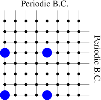
Figure 1: (Color on line) Renormalization procedure in dimension $d=2$. The initial state is the tight-binding Anderson model on a square lattice of size $L^{2}$, with periodic boundary conditions in the two directions. Sites are then iteratively eliminated using the RG rules of Eqs. 9 and 10 until there remains only the four sites corresponding to the large discs, i.e. there are four renormalized on-site energies and four renormalized hoppings at distance $L/2$ per sample.

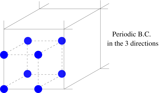
Figure 2: (Color on line) Renormalization procedure in dimension $d=3$. The initial state is the tight-binding Anderson model on a cubic lattice of size $L^{3}$, with periodic boundary conditions in the three directions (here for clarity, the sites of the initial model have not be drawn in contrast to Fig. 1 concerning the case $d=2$ which is more explicit). Sites are then iteratively eliminated using the RG rules of Eqs. 9 and 10 until there remains only the eight sites corresponding to the large discs, i.e. there are eight renormalized on-site energies and twelve renormalized hoppings at distance $L/2$ per sample.

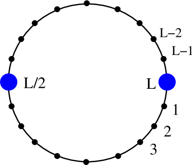
Figure 3: (Color on line) Renormalization procedure for the PRBM model with the ring geometry. Sites are iteratively eliminated using the the RG rules of Eqs. 9 and 10 until there remains only the two sites $L/2$ and $L$ corresponding to the large discs, i.e. there are two renormalized on-site energies and one renormalized hoppings per sample.

The RG rules of Eqs 9 and 10 can be followed numerically from the initial condition given by the model of Eq. 1 under interest. In the following, we describe the sizes and the statistics over the samples that we have studied for the Anderson tight binding model in dimension $d=2$ and $d=3$ and the PRBM model.

II.5.1 Anderson tight binding model in dimension $d=2$ and $d=3$

For the Anderson tight-binding model described in Section II.1.1, we have followed numerically the RG rules starting from an hypercubic lattice of size $L^{d}$ with periodic boundary conditions in all $d$ directions. In each sample, the final state that we analyse is an hypercube of linear size $L/2$, as shown on Figure 1 for $d=2$ and on Figure 2 for $d=3$

(i) in dimension $d=2$, there are four remaining sites per sample as shown on Fig. 1, i.e. there are four renormalized on-site energies and four renormalized couplings at distance $L/2$. We have studied the sizes $L=12,24,36,48,60,72,84,96,108,120$. The corresponding numbers $ns(L)$ of independent samples are of order $n_{s}(L=12)=2.10^{7}$, $n_{s}(L=60)=33.10^{3}$, $n_{s}(L=120)=1150$.

(ii) in $d=3$ there are eight remaining sites per sample as shown on Fig. 2, i.e. there are eight renormalized on-site energies and twelve renormalized couplings at distance $L/2$. We have studied the sizes $L=4,6,8,10,12,14,16,18,20,22,24,26,28,30$. The corresponding numbers $n_{s}(L)$ of independent samples are of order $n_{s}(L=4)=10^{7}$, $n_{s}(L=10)=6.10^{4}$, $n_{s}(L=20)=400$ and $n_{s}(L=30)=24$.

II.5.2 Power-law Random Banded Matrix (PRBM) model

For the PRBM model described in Section II.1.2, we have followed numerically the RG rules up to the final state shown on Fig. 3 containing only the sites $L/2$ and $L$, i.e. in each sample, there are two renormalized on-site energies and one renormalized coupling. We have studied rings of sizes $50\leq L\leq 1800$ with corresponding statistics of $10.10^{8}\geq n_{s}(L)\geq 2400$ independent samples.

III Statistics of renormalized on-site energies

III.1 General properties

We find that the renormalized on-site energies remain finite in all phases (localized, delocalized, critical), and that the histograms ${\cal P}_{L}(\epsilon)$ corresponding to various system sizes $L$ converge towards some stationary distribution ${\cal P}_{\infty}(\epsilon)$ that present the following common properties :

(i) ${\cal P}_{\infty}(\epsilon)$ is symmetric in $\epsilon\to-\epsilon$ (as the initial condition of Eq. 2)

(ii) ${\cal P}_{\infty}(\epsilon)$ has a finite density ${\cal P}_{\infty}(0)$ at its center $\epsilon=0$. After the change of variables to $y\equiv\ln|\epsilon|$, this corresponds to

$$P_{\infty}(y\equiv\ln|\epsilon|)\mathop{\propto}_{y\to-\infty}|\epsilon|=e^{y}$$ (41)

(iii) For $\epsilon\to\pm\infty$, ${\cal P}_{\infty}(\epsilon)$ presents the following power-law decay

$${\cal P}_{\infty}(\epsilon)\mathop{\propto}_{\epsilon\to\pm\infty}\frac{1}{\epsilon^{2}}$$ (42)

After the change of variables to $y\equiv\ln|\epsilon|$, Eq. 42 corresponds to

$$P_{\infty}(y\equiv\ln|\epsilon|)\mathop{\propto}_{y\to+\infty}\frac{1}{|\epsilon|}=e^{-y}$$ (43)

The origin of the power-law of Eq. 42, even when one starts from a bounded distribution in $\epsilon$ as in the tight-binding Anderson model (see Eq. 2), can be understood from the form the RG rule of Eq. 10 which reads at zero energy $E=0$

$$\epsilon_{i}^{new}=\epsilon_{i}-\frac{V_{i,i_{0}}V_{i_{0},i}}{\epsilon_{i_{0}}}$$ (44)

During the first steps of renormalization where the hoppings $V$ are finite, very large renormalized on-site energies are generated when the eliminated on-site energy $\epsilon_{i_{0}}$ is very small. The finite density of ${\cal P}(\epsilon_{i_{0}})$ at $\epsilon_{i_{0}}=0$ yields the power-law decay of Eq. 42 via the change of variable $\epsilon_{i}^{new}\simeq-1/\epsilon_{i_{0}}$ using the standard formula $P_{new}(\epsilon_{i}^{new})d\epsilon_{i}^{new}={\cal P}(\epsilon_{i_{0}})d\epsilon_{i_{0}}$.

In the remaining of this section, we present the histograms we have measured in various cases.

III.2 Results for the square lattice in dimension $d=2$

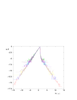
Figure 4: (Color on line) Statistics of renormalized on-site energies $\epsilon$ for the Anderson model on the square lattice in dimension $d=2$ for sizes $12\leq L\leq 120$ (disorder strength $W=40$) : the histograms of $\ln|\epsilon|$ are identical (apart for the cut-off imposed by the statistics over the samples) The left and right slopes of value unity corresponds to Eqs 41 and 43.

On Fig. 4, we show the histograms of the logarithm of the absolute value of the renormalized on-site energy $\epsilon$ for various sizes $12\leq L\leq 120$ : apart from the cut-offs in the tails imposed by different statistics over the samples, these histograms coincide. This shows that the convergence towards the stationary distribution ${\cal P}_{\infty}(\epsilon)$ is quite rapid : starting from the initial condition of Eq. 2, our results for the smallest size $l=12$ have already ’converged’ towards the final- and very different- distribution of Figure 4. On Fig. 4, the slope of the left tail is of order $+1$ in agreement with Eq. 41, and the slope of the right tail is of order $-1$ in agreement with Eq. 43.

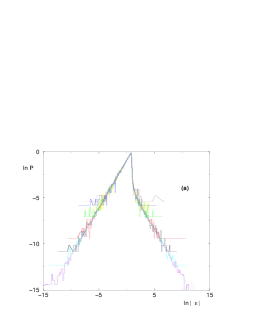
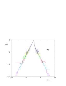
Figure 5: (Color on line) Statistics of renormalized on-site energies $\epsilon$ for the Anderson model on the cubic lattice in dimension $d=3$ for sizes $4\leq L\leq 20$ (a) Histograms of $\ln|\epsilon|$ in the localized phase ($W=40$) (b) Histograms of $\ln|\epsilon|$ at criticality ($W_{c}=16.5$)

III.3 Results for the cubic lattice in dimension $d=3$

Our data for the Anderson tight binding model in $d=3$ are shown on Fig. 5 : both in the localized phase and at criticality, the convergence in $L$ towards the stationary distribution ${\cal P}_{\infty}(\epsilon)$ is still rapid, and the measured tails are again in agreement with Eqs 41 and 43. It turns out that for a given disorder value, our numerical results concerning ${\cal P}_{\infty}(\epsilon)$ seem to coincide for $d=2$ and $d=3$ (Fig. 4 and Fig. 5 (a) corresponding to $W_{d}=40$) : the reasons of this coincidence are not clear to us, since the initial coordinence of sites clearly depends on the dimension $d$.

III.4 Results for the PRBM model

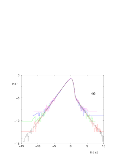
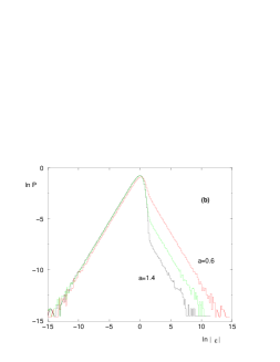
Figure 6: (Color on line) Statistics of renormalized on-site energies $\epsilon$ in the PRBM model of parameter $b=0.1$ (a) The histograms of $\ln|\epsilon|$ at criticality $a=1$ for various sizes $L=100,200,400,600,800$ are identical (apart for the cut-off imposed by the statistics over the samples). (b) Comparison of the stationary distributions in the localized phase ($a=1.4$), at criticality ($a=1$) and in the delocalized phase ($a=0.6$). The left and right slopes of value unity corresponds to Eqs 41 and 43.

The properties found above for Anderson tight-binding models seem to be valid for more general Anderson models of the form of Eq. 1. As an example, we show on Fig. 6 our data concerning the PRBM model described in section II.1.2. The histograms of renormalized energies converge rapidly towards their limit. The stationary distribution presents the tails of Eqs 41 and 43 in all phases (localized, critical, delocalized).

III.5 Consequences

In conclusion, the renormalized on-site energies remain finite random variables in all phases (localized, critical, delocalized). As a consequence, the behavior of the two-point Landauer transmission of Eq. 31 is determined by the properties of the renormalized hoppings

(i) in the delocalized phase, both the renormalized hopping and the two-point transmission will remain random finite variables.

(ii) in the localized phase and at criticality where the two-point transmission decays with the distance, its decay will be directly related to the decay of the renormalized hopping via

$$\ln T(E=0)\simeq\ln V_{AB}^{2}+{\rm finite}$$ (45)

In the following, we discuss the statistics of renormalized hoppings in the localized phase and at criticality, in relation with the statistics of two-point transmission.

IV Statistics of renormalized hoppings in the localized phase

IV.1 Universality class of the directed polymer in a random medium

In dimension $d=1$, the transfer matrix formulation of the Schrödinger equation yields a log-normal distribution for the Landauer transmission [27, 28]

$$\ln T_{L}^{(d=1)}\mathop{\propto}_{L\to\infty}-\frac{L}{\xi_{loc}}+L^{1/2}u$$ (46)

The leading non-random term is extensive in $L$ and involves the localization length $\xi_{loc}$. The subleading random term is of order $L^{1/2}$, and the random variable $u$ of order $O(1)$ is Gaussian distributed as a consequence of the Central Limit theorem. Although it has been very often assumed and written that this log-normal distribution persists in the localized phase in dimension $d=2,3$, theoretical arguments [16, 17] and recent numerical calculations [18] are in favor of the following scaling form for the logarithm of the transmission

$$\ln T_{L}^{(d)}\mathop{\propto}_{L\to\infty}-\frac{L}{\xi_{loc}}+L^{\omega(d)}u$$ (47)

where the exponent $\omega(d)$ depends on the dimension $d$ and coincides with the droplet exponent characterizing the strong disorder phase of the directed polymer in a random medium of dimension $1+(d-1)$ (see the review [29] on directed polymers). The probability distribution of the rescaled variable $u$ is not Gaussian but is determined by the directed polymer universality class (see [18] where its distribution in $d=2$ is shown to coincide with the exactly known Tracy-Widom distribution for the directed polymer in $1+1$).

The arguments in favor of the same universality class can be decomposed in two steps [16, 17, 18] :

(i) in the localized phase of Anderson localization in dimension $d$, the transmission decays exponentially with the length, and thus directed paths completely dominate asymptotically over non-directed paths. In dimension $d=2$, the dominance of a narrow channel can be seen on Figs 10 and 11 of Ref [30].

(ii) these directed paths of the Anderson model have weights that are random both in magnitude and sign, but it turns out that the directed polymer model which is usually defined with random positive weights (Boltzmann weights) keeps the same exponents in the presence of complex weights (see section 6.3 of the review [29]).

In conclusion, from the relation of Eq. 45, we expect that the renormalized hoppings will present the same statistics as the Landauer transmission of Eq. 47

$$\ln V_{L}\simeq-\frac{L}{\xi_{loc}}+L^{\omega(d)}u+...$$ (48)

To check this relation, we have measured the averaged value and the variance of the logarithm of the renormalized hoppings in dimension $d=2,3$.

IV.2 Results for the square lattice in dimension $d=2$

Figure 7: Statistics of the typical renormalized hopping in $d=2$ where only the localized phase exists (the data shown correspond to the disorder strength $W=40$) (a) Typical exponential decay : $\overline{\ln V_{L}}$ is linear in $L$ and the slope represents the inverse of the localization length $\xi_{loc}$ (Eq. 48). (b) The fluctuation term $\Delta(\ln V_{L})$ grows as $L^{\omega}$ (Eq. 48) with $\omega(d=2)\simeq 0.33$.

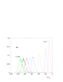
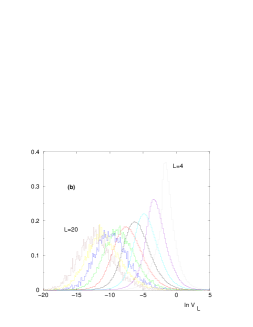
Figure 8: (Color on line) Histograms of the logarithm of the renormalized hopping $\ln V_{L}$ for various lengths $L$ in the localized phase (for the disorder strength $W=40$ (a) in dimension $d=2$ (b) in dimension $d=3$

In dimension $d=2$, only the localized phase exists. On Fig. 7 (a), we show the typical exponential decay corresponding to a finite localization length $\xi_{loc}$ in Eq. 48. On Fig. 7 (b), we show the amplitude $\Delta(\ln V_{L})$ of the random term in Eq. 48 : the three parameters fit $\Delta(\ln V_{L})=a_{0}L^{\omega(d=2)}+a_{1}$ yields the value

$$\omega(d=2)\simeq 0.33$$ (49)

in agreement with the exact result [31, 32, 33, 34]

$$\omega_{DP}(1+1)=\frac{1}{3}$$ (50)

for the directed polymer in a random medium of dimension $1+1$. On Fig. 8 (a), we show the histograms of $(\ln V_{L})$ for various sizes $L$ : as $L$ grows, the maximum moves linearly while the width grows as $L^{\omega}$.

IV.3 Results for the cubic lattice in dimension $d=3$

Figure 9: Statistics of the typical renormalized hopping in $d=3$ in the localized phase ($W=40$) (a) $\overline{\ln V_{L}}$ as a function of $L$ : the slope represents the inverse of the localization length $\xi_{loc}$ (Eq. 48) (b) The fluctuation term $\Delta(\ln V_{L})$ grows as $L^{\omega}$ (Eq. 48) with $\omega(d=3)\simeq 0.24$.

In dimension $d=3$, the localized phase exists in the domain $W>W_{c}\simeq 16.5$ for the disorder strength (Eq. 3). The data shown on Fig. 9 corresponds to the disorder strength $W=40$. The histograms of $(\ln V_{L})$ for various sizes $L$ are shown on Fig. 8 (b). On Fig. 9 (a), the typical exponential decay found corresponds to a finite localization length $\xi_{loc}$ in Eq. 48. On Fig. 9 (b), the amplitude $\Delta(\ln V_{L})$ of the random term in Eq. 48 can be fitted by the form $\Delta(\ln V_{L})=a_{0}L^{\omega(d=3)}+a_{1}$ that yields the value

$$\omega(d=3)\simeq 0.24$$ (51)

in agreement with the measures of the droplet exponent $\omega_{DP}(1+2)\simeq 0.244$ obtained for the directed polymer in a random medium of dimension $1+2$ in various Refs [35, 36, 37, 38, 39].

V Statistics of renormalized hoppings at criticality

V.1 Expected multifractal statistics

At criticality, the statistics of the two-point transmission is multifractal [19, 20, 21] : the critical probability distribution of the two-point transmission $T_{L}$ takes the form

$${\rm Prob}\left(T_{L}\sim L^{-\kappa}\right)dT\mathop{\propto}_{L\to\infty}L^{\Phi(\kappa)}d\kappa$$ (52)

where the multifractal spectrum $\Phi(\kappa)$ exist only for $\kappa\geq 0$ (as a consequence of the physical bound $T_{L}\leq 1$) and is related to the singularity spectrum $f(\alpha)$ of eigenfunctions via

$$\Phi(\kappa\geq 0)=2\left[f(\alpha=d+\frac{\kappa}{2})-d\right]$$ (53)

At criticality the decay of the two-point transmission is directly related to the decay of the renormalized hopping via Eq. 45. As a consequence, what is known about the statistics of the two-point transmission at criticality can be translated for the renormalized hoppings. The probability distribution of the renormalized hopping $V_{L}$ at scale $L$ takes the form

$${\rm Prob}\left(|V_{L}|\sim L^{-\rho}\right)dV\mathop{\propto}_{L\to\infty}L^{H(\rho)}d\rho$$ (54)

where

$$H(\rho\geq 0)=\Phi(2\rho)=2\left[f(\alpha=d+\rho)-d\right]$$ (55)

In particular, the typical exponent $\rho_{typ}$ characterizing the typical decay

$$\overline{\ln V_{L}}\mathop{\simeq}_{L\to+\infty}-\rho_{typ}\ln L$$ (56)

is related to the typical exponent $\kappa_{typ}$ of the two-point transmission and to the typical exponent $\alpha_{typ}$ of the singularity spectrum via

$$\rho_{typ}=\frac{\kappa_{typ}}{2}=\alpha_{typ}-d$$ (57)

V.2 Results for the cubic lattice in dimension $d=3$

Figure 10: Statistics of the typical renormalized hopping in $d=3$ at criticality ($W=16.5$) (a) $\overline{\ln V_{L}}$ as a function of $\ln L$ for bulk sites (see Fig. 2) : the measured slope $\rho_{typ}\simeq 1.05$ represents the typical exponent of Eq. 56. (b) $\overline{\ln V_{L}^{surf}}$ as a function of $\ln L$ for surface sites (see Fig. 11) : the measured slope $\rho_{typ}^{surf}\simeq 1.6$ represents the typical exponent of Eq. 60.

The typical exponent $\rho_{typ}$ of Eq. 56 is measured from the data of Fig. 10 (a)

$$\rho_{typ}\simeq 1.05$$ (58)

Via Eq. 57, this value is in agreement with the numerical measures of order [40, 41]

$$\alpha_{typ}\simeq 4$$ (59)

for the exponent $\alpha_{typ}$ concerning the singularity spectrum of eigenfunctions.

Of course, beyond this typical exponent, one could in principle extract from our numerical data, results on the whole multifractal spectrum. However, our numerical means in $d=3$ are limited to rather small sizes and small statistics (see the section II.5.1) in comparison with the exact diagonalization calculations of Refs [41]. As a consequence, our numerical results seem sufficient to measure the correct typical exponent, as shown above, but we believe that they are not sufficient to measure correctly the rare events that are necessary to obtain a reliable multifractal spectrum. It may be that in the future, more ’professional numericians’ will be able to transform the present renormalization approach into a competitive numerical method to measure the multifractal spectrum, but this is clearly beyond our numerical means.

V.3 Renormalized hopping between two surface points in dimension $d=3$

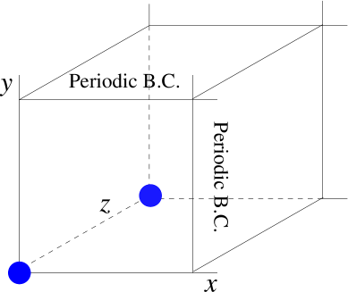
Figure 11: (Color on line) Renormalization procedure in dimension $d=3$ to measure the renormalized hopping $V_{L}^{surf}$ between two boundary sites. The initial state is the tight-binding Anderson model on a cubic lattice of size $L^{3}$, with periodic boundary conditions in two directions $x$ and $y$ and free boundary conditions in the third direction $z$. Sites are then iteratively eliminated using the the RG rules of Eqs. 9 and 10 until there remains only the two surface sites corresponding to the large discs.

At criticality, points lying on the boundaries are characterized by a specific multifractal spectrum $f_{surf}(\alpha)$, different from the bulk spectrum $f(\alpha)$ [42, 43, 44]. These surface critical properties are particularly interesting in Anderson localization models where it is more natural to attach leads to boundary sites rather than bulk sites. We have thus considered the renormalization procedure depicted on Fig. 11 to measure the statistical properties of the renormalized hoppings between two surface points. The typical behavior shown on Fig. 10 (b)

$$\overline{\ln V_{L}^{surf}}\mathop{\simeq}_{L\to+\infty}-\rho_{typ}^{surf}\ln L$$ (60)

corresponds to an exponent of order

$$\rho_{typ}^{surf}\simeq 1.6$$ (61)

clearly distinct from its bulk analog of Eq. 58.

Via Eq. 57, we expect that this value corresponds to

$$\alpha_{typ}^{surf}=d+\rho_{typ}^{surf}\simeq 4.6$$ (62)

for the typical exponent $\alpha_{typ}^{surf}$ of the surface singularity spectrum of eigenfunctions. In contrast with the bulk case, we are not aware of any direct measure of $\alpha_{typ}^{surf}$ in the literature to make some comparison. As explained at the end of section V.2, we believe that our numerical means are not sufficient to measure correctly the rare events to obtain the full multifractal spectrum around this typical value. However, we expect that our result for the typical exponent is reliable (as shown above for the bulk case), and will be confirmed in the future whenever the surface multifractal spectrum will be measured via the powerful exact diagonalization techniques of [41].

From Eq. 57, we also expect that the two-point transmission in $d=3$ between two surface points involves the typical exponent

$$\kappa_{typ}^{surf}=2\rho_{typ}^{surf}\simeq 3.2$$ (63)

V.4 Results for the PRBM model

For the PRBM model, we have studied in detail the multifractal properties of the two-point transmission in our previous works [20, 21]. Since the statistics of renormalized hoppings can be directly deduced from them via Eqs 55, we refer the interested reader to [20, 21] where we have measured multifractal spectra at criticality $a=1$ for various values of the parameter $b$.

VI Conclusion

In this paper, we have revisited the exact real-space renormalization procedure at fixed energy proposed by Aoki [13, 14, 15] for Anderson localization models. We have presented detailed numerical results concerning the statistical properties of the renormalized on-site energies $\epsilon$ and of the renormalized hoppings $V$ as a function of the linear size $L$ for the Anderson tight-binding models in dimension $d=2$ where only the localized phase exists, and in dimension $d=3$ where there exists an Anderson localization transition. Our main conclusions are the following :

(a) the renormalized on-site energies $\epsilon$ remain finite in the localized phase in $d=2,3$ and at criticality ($d=3$), with a finite density at $\epsilon=0$ and a power-law decay $1/\epsilon^{2}$ at large $|\epsilon|$.

(b) in the localized phase in dimension $d=2,3$, the statistics of renormalized couplings belongs to the universality class of the directed polymer in a random medium of dimension $1+(d-1)$, in agreement with [16, 17, 18].

(c) at criticality, the statistics of renormalized hoppings $V$ is multifractal, in direct correspondence with the multifractality of individual eigenstates and of two-point transmissions. In particular, our measure $\rho_{typ}\simeq 1$ for the exponent governing the typical decay $\overline{{\rm ln}\ V_{L}}\simeq-\rho_{typ}\ {\rm ln}L$, is in agreement with previous numerical measures of $\alpha_{typ}=d+\rho_{typ}\simeq 4$ for the singularity spectrum $f(\alpha)$ of individual eigenfunctions. We have also measured the corresponding critical surface properties.

In conclusion, we have shown that the large scale properties of Anderson localization models actually emerge from the simple real-space RG rules of Eqs 9 and 10 which preserve exactly the Green functions of the remaining sites.

References

- [1] Th. Niemeijer, J.M.J. van Leeuwen, ”Renormalization theories for Ising spin systems” in Domb and Green Eds, ”Phase Transitions and Critical Phenomena” (1976); T.W. Burkhardt and J.M.J. van Leeuwen, “Real-space renormalizations”, Topics in current Physics, Vol. 30, Spinger, Berlin (1982); B. Hu, Phys. Rep. 91, 233 (1982).
- [2] A.A. Migdal, Sov. Phys. JETP 42, 743 (1976) ; L.P. Kadanoff, Ann. Phys. 100, 359 (1976).
- [3] A.N. Berker and S. Ostlund, J. Phys. C 12, 4961 (1979).
- [4] M. Kaufman and R. B. Griffiths, Phys. Rev. B 24, 496 (1981); R. B. Griffiths and M. Kaufman, Phys. Rev. B 26, 5022 (1982).
- [5] P.W. Anderson, Phys. Rev. 109, 1492 (1958).
- [6] D.J. Thouless, Phys. Rep. 13, 93 (1974) ; D.J. Thouless, in “Ill Condensed Matter” (Les Houches 1978), Eds R Balian, R Maynard and G Toulouse, North-Holland, Amsterdam (1979).
- [7] B. Souillard, in “ Chance and Matter” (Les Houches 1986), Eds J Souletie, J Vannimenus and R Stora, North-Holland, Amsterdam (1987).
- [8] I.M. Lifshitz, S.A. Gredeskul and L.A. Pastur, “Introduction to the theory of disordered systems” (Wiley, NY, 1988).
- [9] B. Kramer and A. MacKinnon, Rep. Prog. Phys. 56, 1469 (1993).
- [10] M. Janssen, Phys. Rep. 295, 1 (1998).
- [11] P. Markos, Acta Physica Slovaca 56, 561 (2006).
- [12] F. Evers and A.D. Mirlin, Rev. Mod. Phys. 80, 1355 (2008).
- [13] H. Aoki, J. Phys. C 13, 3369 (1980).
- [14] H. Aoki, Physica A 114, 538 (1982).
- [15] H. Kamimura and H. Aoki, “The physics of interacting electrons and disordered systems”, Clarendon Press Oxford (1989).
- [16] V.L. Nguyen, B.Z. Spivak and B.I. Shklovskii, JETP Lett. 41, 43 (1985); V.L. Nguyen, B.Z. Spivak and B.I. Shklovskii, Sov. Phys. JETP 62,, 1021 (1985).
- [17] E. Medina, M. Kardar, Y. Shapir and X.R. Wang, Phys. Rev. Lett. 62, 941 (1989); E. Medina and M. Kardar, Phys. Rev. B 46, 9984 (1992).
- [18] J. Prior, A.M. Somoza and M. Ortuno, Phys. Rev. B 72, 024206 (2005); A.M. Somoza, J. Prior and M. Ortuno, Phys. Rev. B 73, 184201 (2006); A.M. Somoza, M. Ortuno and J. Prior, Phys. Rev. Lett. 99, 116602 (2007).
- [19] M. Janssen, M. Metzler and M.R. Zirnbauer, Phys. Rev. B 59, 15836 (1999).
- [20] C. Monthus and T. Garel, Phys. Rev. B 79, 205120 (2009).
- [21] C. Monthus and T. Garel, arxiv:0904.4547.
- [22] A.D. Mirlin et al, Phys. Rev. E 54, 3221 (1996).
- [23] F. Evers and A. D. Mirlin Phys. Rev. Lett. 84, 3690 (2000); A.D. Mirlin and F. Evers, Phys. Rev. B 62, 7920 (2000).
- [24] E. Cuevas, V. Gasparian and M. Ortuno, Phys. Rev. Lett. 87, 056601 (2001).
- [25] E. Cuevas et al, Phys. Rev. Lett. 88, 016401 (2001).
- [26] I. Varga, Phys. Rev. B 66, 094201 (2002).
- [27] P. W. Anderson, D. J. Thouless, E. Abrahams and D. S. Fisher Phys. Rev. B 22, 3519 (1980).
- [28] J.M. Luck, “Systèmes désordonnés unidimensionnels” , Alea Saclay, Gif-sur-Yvette, France (1992).
- [29] T. Halpin-Healy and Y.C. Zhang, Phys. Rep. 254 (1995) 215.
- [30] P. Markos, arxiv:0807.2531.
- [31] D. A. Huse, C. L. Henley, and D. S. Fisher, Phys. Rev. Lett. 55, 2924 (1985).
- [32] M. Kardar, Nucl. Phys. B 290 582 (1987).
- [33] K. Johansson, Comm. Math. Phys. 209 (2000) 437.
- [34] M. Prahofer and H. Spohn, Physica A 279, 342 (2000) ; M. Prahofer and H. Spohn, Phys. Rev. Lett. 84, 4882 (2000) ; M. Prahofer and H. Spohn, J. Stat. Phys. 108, 1071 (2002).
- [35] L.H. Tang, B.M. Forrest and D.E. Wolf, Phys. Rev. A 45 (1992) 7162.
- [36] T. Ala-Nissila, T. Hjelt, J.M. Kosterlitz and V. Venalainen, J. Stat. Phys. 72 (1993) 207.
- [37] T. Ala-Nissila, Phys. Rev. Lett. 80 (1998) 887 ; J.M. Kim, Phys. Rev. Lett. 80 (1998) 888.
- [38] E. Marinari, A. Pagnani and G. Parisi, J Phys. A 33 (2000) 8181 ; E. Marinari, A. Pagnani and G. Parisi and Z. Racz, Phys. Rev. E 65 (2002) 026136.
- [39] C. Monthus and T. Garel, Phys. Rev. E 73 , 056106 (2006); C. Monthus and T. Garel, Phys. Rev. E 74, 051109 (2006).
- [40] A. Mildenberger, F. Evers and A.D. Mirlin, Phys. Rev. B 66, 033109 (2002).
- [41] L.J. Vasquez, A. Rodriguez and R.A. Romer, Phys. Rev. B 78, 195106 (2008); A. Rodriguez, L.J. Vasquez and R.A. Romer, Phys. Rev. B 78, 195107 (2008); A. Rodriguez, L.J. Vasquez and R.A. Romer, Phys. Rev. Lett. 102, 106406 (2009).
- [42] A. R. Subramaniam, I. A. Gruzberg, A. W. W. Ludwig, F. Evers, A. Mildenberger, and A. D. Mirlin, Phys. Rev. Lett. 96, 126802 (2006).
- [43] A. Mildenberger, A. R. Subramaniam, R. Narayanan, F. Evers, I. A. Gruzberg, and A. D. Mirlin, Phys. Rev. B 75, 094204 (2007).
- [44] H. Obuse, A. R. Subramaniam, A. Furusaki,I. A. Gruzberg, and A. W. W. Ludwig, Phys. Rev. Lett. 101, 116802 (2008).