A SURVEY OF $z\sim 6$ QUASARS IN THE SDSS DEEP STRIPE. II. DISCOVERY OF SIX QUASARS AT $z_{\rm AB}>21$

Abstract

We present the discovery of six new quasars at $z\sim 6$ selected from the Sloan Digital Sky Survey (SDSS) southern survey, a deep imaging survey obtained by repeatedly scanning a stripe along the celestial equator. The six quasars are about two magnitudes fainter than the luminous $z\sim 6$ quasars found in the SDSS main survey and one magnitude fainter than the quasars reported in Paper I (Jiang et al., 2008). Four of them comprise a complete flux-limited sample at $21<z_{AB}<21.8$ over an effective area of 195 deg². The other two quasars are fainter than $z_{AB}=22$ and are not part of the complete sample. The quasar luminosity function at $z\sim 6$ is well described as a single power law $\Phi(L_{1450})\propto L_{1450}^{\beta}$ over the luminosity range $-28<M_{1450}<-25$. The best-fitting slope $\beta$ varies from –2.6 to –3.1, depending on the quasar samples used, with a statistical error of 0.3–0.4. About 40% of the quasars discovered in the SDSS southern survey have very narrow Ly$\alpha$ emission lines, which may indicate small black hole masses and high Eddington luminosity ratios, and therefore short black hole growth time scales for these faint quasars at early epochs.

1 INTRODUCTION

High-redshift quasars serve as cosmological probes for studying the early universe. In recent years, about 40 quasars at $z\sim 6$ have been discovered; the most distant ones are at $z\sim 6.4$ (Fan et al., 2006; Willott et al., 2007). They harbor billion-solar-mass black holes, and thus are essential in understanding black hole accretion and galaxy formation in the first billion years of cosmic time. Most of the known quasars at $z\sim 6$ were discovered from $\sim 8000$ deg² of imaging data of the Sloan Digital Sky Survey (SDSS; York et al., 2000). These luminous quasars ($z_{AB}\leq 20$, $M_{1450}\sim-27$) were selected as $i$-dropout objects using optical colors; follow-up near-infrared (NIR) photometry and optical spectroscopy were used to distinguish against late-type dwarfs (e.g. Fan et al., 2001a). Several other high-redshift quasars have also been discovered based on their infrared or radio emission (e.g. Cool et al., 2006; McGreer et al., 2006).

Currently ongoing surveys of $z\sim 6$ quasars include the UKIRT Infrared Deep Sky Survey (UKIDSS; Warren et al., 2007) and the Canada-France High-redshift Quasar Survey (CFHQS; Willott et al., 2005). The UKIDSS survey is being carried out in the $YJHK$ bands using the Wide Field Camera (Casali et al., 2007) on the 3.8 m UKIRT telescope. It will survey 7500 square degrees of the northern sky. The resulting NIR data together with the SDSS multicolor optical data can be used to select high-redshift quasar candidates. The UKIDSS team has found two quasars at $z\sim 6$ (Venemans et al., 2007; Mortlock et al., 2008). These quasars are fainter than $z_{AB}=20$, the magnitude selection limit that the SDSS team used (Fan et al., 2006). The CFHQS survey is an optical imaging survey of $\sim 550$ square degrees in the $griz$ bands on the Canada-France-Hawaii Telescope (Willott et al., 2009). The survey is about two magnitudes deeper than the SDSS wide survey. The CFHQS team has found 10 quasars at $z\sim 6$ to date, including the most distant quasar known at $z=6.43$ (Willott et al., 2007, 2009).

This paper is the second in a series presenting $z\sim 6$ quasars selected from the SDSS southern survey, a deep imaging survey obtained by repeatedly scanning a 300 deg² stripe along the celestial equator. In Jiang et al. (2008, hereafter Paper I) we reported the discovery of five quasars at $5.85\leq z\leq 6.12$ in 260 deg² of the deep stripe. Together with another quasar known in this region (Fan et al., 2004), they constructed a complete flux-limited quasar sample at $20<z_{AB}<21$. Based on the combination of this sample, the luminous quasar sample from $\sim 8000$ deg² of SDSS, and the Cool et al. (2006) sample, we found a steep slope at the bright end of the quasar luminosity function (QLF) at $z\sim 6$. In this paper we present the discovery of six new quasars in the SDSS deep stripe. All six quasars are about one magnitude fainter than those reported in Paper I, or two magnitudes fainter than the luminous SDSS quasars. With these new quasars, we can measure the QLF over three magnitudes. The basic procedures of candidate selection, follow-up observations, and data reduction are similar to the procedures used in Paper I.

The structure of the paper is as follows. Section 2 briefly introduces the construction of the SDSS co-added imaging data. Section 3 describes our selection criteria and follow-up observations of quasar candidates. We present the six new quasars in Section 4 and discuss the QLF at $z\sim 6$ in Section 5. We summarize the paper in Section 6. Throughout the paper we use a $\Lambda$-dominated flat cosmology with H${}_{0}=70$ km s^-1 Mpc^-1, $\Omega_{m}=0.3$, and $\Omega_{\Lambda}=0.7$ (Spergel et al., 2007).

2 CONSTRUCTION OF THE SDSS CO-ADDED IMAGING DATA

2.1 SDSS Deep Imaging Data

The SDSS was an imaging and spectroscopic survey of the sky (York et al., 2000) using a dedicated wide-field 2.5 m telescope (Gunn et al., 2006) at Apache Point Observatory. Imaging was carried out in drift-scan mode using a 142 mega-pixel camera (Gunn et al., 1998) which gathered data in five broad bands, $ugriz$, spanning the range from 3000 to 10,000 Å (Fukugita et al., 1996), on moonless photometric (Hogg et al., 2001) nights of good seeing. The effective exposure time was 54 s. The images were processed using specialized software (Lupton et al., 2001), and were photometrically (Tucker et al., 2006; Ivezić et al., 2004) and astrometrically (Pier et al., 2003) calibrated using observations of a set of primary standard stars (Smith et al., 2002) on a neighboring 20-inch telescope. All magnitudes are roughly on an AB system (Oke & Gunn, 1983), and use the asinh scale described by Lupton et al. (1999).

The primary goal of the SDSS imaging survey was to scan 8500 deg² of the north Galactic cap (hereafter referred to as the SDSS main survey). In addition to the main survey, SDSS also conducted a deep survey by repeatedly imaging a 300 deg² area on the celestial equator in the south Galactic cap in the fall (hereafter referred to as the SDSS deep survey; Abazajian et al., 2009). This deep stripe (also called Stripe 82; see Stoughton et al. 2002) spans $\rm 20^{h}<R.A.<4^{h}$ and $\rm-1.25\arcdeg<decl.<1.25\arcdeg$. The multi-epoch images, when coadded, allow the selection of much fainter quasars than the SDSS main survey. We used the 10-run co-added data (constructed in 2005) in Paper I and found five $z\sim 6$ quasars with $20<z_{AB}<21$ in this area.

The construction of the co-added images is close, but not identical, to that of Annis et al. (in preparation), Paper 1, and Abazajian et al. (2009). We used $50\sim 60$ scans from the SDSS deep southern stripe, restricting ourselves to fields with $r$-band seeing less than $2\arcsec$ and $r$-band sky fainter than 19.5 mag/arcsec². Because our selection algorithm uses only $r$, $i$, and $z$-band photometry, we did not co-add the $u$ and $g$-band data. The input images are the SDSS corrected frames (or fpC images). Each input image was calibrated to a standard SDSS zero point and weighted on a field-by-field basis with

$$w=\frac{T}{\rm FWHM^{2}\,\sigma^{2}}\,,$$ (1)

where $T$ is the transparency as measured by the relative zero point of the image, FWHM is the full width at half maximum of the PSF, and $\sigma^{2}$ is the variance of the sky. We did not use mask files in the weight map. After sky background was estimated and subtracted, the images were mapped onto a uniform rectangular output astrometric grid using a modified version of the registration software SWARP (Bertin et al., 2002). The weight maps were subjected to the same mapping. The final co-added images are about two magnitudes deeper than the SDSS single-run data. The median seeing of the co-adds as measured in the $z$ band is $\sim 1.2\arcsec$.

2.2 Photometry

The co-added images included in the SDSS DR7 (Abazajian et al., 2009) were run through the SDSS photometric pipeline PHOTO. For a variety of technical reasons, we could not do the same for our co-added images, so we used SExtractor (Bertin & Arnouts, 1996) instead of PHOTO to do photometry. For each field, the photometry of the three ($riz$) co-added images includes the following steps. First we detected sources in the $z$-band image. We used aperture photometry with an aperture (diameter) size $3\arcsec$ (or 7.5 pixels), 2.5 times the typical PSF FWHM. We then used SExtractor double-image mode to do photometry in the $r$ and $i$ bands at the positions of the $z$-band detections, using the same $3\arcsec$ aperture. Finally we applied aperture correction to a large aperture using standard stars in the same field (Ivezić et al., 2007), and corrected for Galactic extinction using Schlegel, Finkbeiner, & Davis (1998).

3 CANDIDATE SELECTION AND FOLLOW-UP OBSERVATIONS

3.1 Quasar Selection Procedure

Because of the rarity of high-redshift quasars and overwhelming number of contaminants, our selection procedure of faint $z>5.7$ quasars contains several steps. It is similar to the procedure used in Paper I:

1. Select $i$-dropout sources from the SDSS co-added data. Objects with $i_{AB}-z_{AB}>2.2$ and $z_{AB}<21.8$ that were not detected in the $r$ band were selected as $i$-dropout objects. The color cut separates high-redshift quasars from the majority of stellar objects (e.g. Fan et al., 2001a); $z_{AB}=21.8$ corresponds roughly to a 10 $\sigma$ detection, i.e., magnitude errors of $\sim 0.1$ mag.

2. Remove false $i$-dropout objects. All $i$-dropout objects were visually inspected, and false detections were deleted from the list of candidates. In Paper I, the majority of the contaminants were cosmic rays. In this paper we incorporated a sigma clipping algorithm into SWARP during the pixel co-addition, which removes almost all cosmic rays as well as high proper-motion objects. The remaining cosmic rays were recognized by visually comparing the individual multi-epoch images making up the co-adds. Roughly 140 objects with $z_{AB}<21.8$ remained at this stage.

3. NIR photometry of $i$-dropout objects. We then carried out $J$-band photometry of the $i$-dropout objects selected from the previous step. The details of the NIR observations are described in Section 3.2 below. Using the $i-z$ versus $z-J$ color-color diagrams (Figure 2 in Paper I), high-redshift quasar candidates were separated from brown dwarfs. We selected quasars with the following criteria,

   $$i-z>2.2\ \ {\rm and}\ \ z-J<0.5\,(i-z)+0.5\,.$$ (2)

   We also carried out $Y$-band photometry for some candidates, especially those that were barely detected in the $i$ band and thus have large $i-z$ uncertainties. The $Y$ band fills in the gap between $z$ and $J$, and the $Y-J$ color efficiently separates brown dwarfs from high-redshift quasars, since most dwarfs from early L to late T have $Y-J$ colors close to 1, while $z\sim 6$ quasars usually have $Y-J$ colors below 0.8. So we applied the criterion

   $$Y-J<0.8$$ (3)

   to the candidates for which we had $Y$-band photometry. 25 objects remained at this stage. Note that the $i$ and $z$ magnitudes are AB magnitudes and the $Y$ and $J$ magnitudes are Vega-based magnitudes.

4. Follow-up spectroscopy of quasar candidates. The final step is to carry out optical spectroscopic observations of quasar candidates to identify high-redshift quasars. The details of the spectroscopic observations are described in Section 3.2.

We applied the above selection criteria to the data in the range $\rm 310\arcdeg<R.A.<30\arcdeg$. The data contain some “holes” in which the coadded images were not available. The effective area is $\sim 195$ deg². In addition to this main search of quasars down to $z_{AB}=21.8$, we also selected 35 $i$-dropout objects with $22.0<z_{AB}<22.3$ in the range $\rm 0\arcdeg<R.A.<55\arcdeg$. Eight of them passed the criteria of the third step. This is to test how deep one can reach with the SDSS co-added images.

3.2 NIR Photometry and Optical Spectroscopic Observations

We obtained $J$ and $Y$-band photometry of the $i$-dropouts using the NOAO SQIID infrared camera (Ellis et al., 1993) on the 4 m Telescope at KPNO and the NIR imager PANIC (Martini et al., 2004) on the Magellan telescopes at Chile. The SQIID observations were made in 2007 October. SQIID produces simultaneous images of the same field in the $J$, $H$, and $K$ bands. The pixel size is $0.39\arcsec$ and the field of view (FOV) is about $3\arcmin\times 3\arcmin$. We used a $2\times 2$, $2\times 3$, or $2\times 4$ dither pattern of $15\arcsec$ offsets to obtain good sky subtraction and to remove cosmic rays. The exposure time at each dither position was 2 min, which was the co-addition of 8 separate 15 s exposures. The total integration time on individual targets was therefore 8, 12, or 16 min. The SQIID data were reduced using the package ‘upsqiid’ within IRAF. Briefly, for each object the SQIID data were dark-subtracted and flat-fielded. The flat field was the median of 30–50 science images taken at the same night. The flat field was also used to create a bad pixel mask. After bad pixels were repaired by interpolation, the sky background was measured and subtracted from the science images. Finally the processed science data were combined to one co-added image. A few standard stars were taken during the night to measure the aperture correction and to carry out absolute flux calibration.

PANIC observations in $Y$ and $J$ were made in 2007 October and 2008 August. The pixel size of PANIC is $0.125\arcsec$ and the FOV is about $2\arcmin\times 2\arcmin$. We used a 5-position dither pattern with a dither offset of $10\arcsec$. The exposure time at each dither position varied from 60 to 120 s, so the total integration time on individual targets was 5–10 min. The PANIC data were reduced using the IRAF PANIC package. The basic procedure is similar to what we did for the SQIID data. After a dark was subtracted and a linearity correction was applied, the frames of each object were flat-fielded. The flat field was created from twilight images. Then the sky background was measured and subtracted. The processed images were corrected for distortion and were combined.

After NIR photometry of the $i$-dropouts, 25 objects with $z_{AB}<21.8$ and 8 objects with $z_{AB}>22$ satisfied the criteria in Section 3.1. Optical spectroscopy of these candidates was carried out using the the Red Channel spectrograph on the MMT in 2007 November and 2008 October. The observations were performed in long-slit mode with a spectral resolution of $\sim 10$ Å. The exposure time for each target was 15–30 min, which was sufficient to identify our candidates under normal weather conditions on the MMT. If a target was identified as a quasar, several additional exposures were taken to improve the spectral quality. The quasar data were reduced using standard IRAF routines.

4 DISCOVERY OF SIX QUASARS AT $z\sim 6$

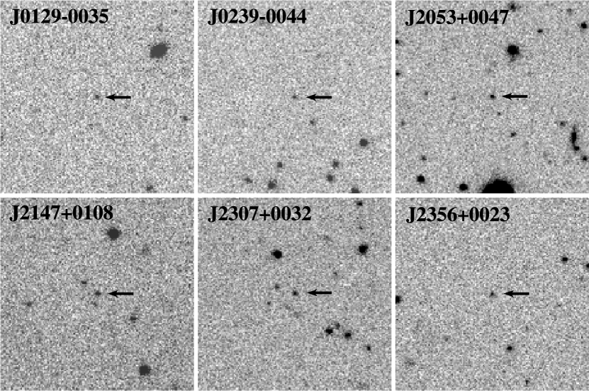
Figure 1: The $z$-band finding charts of the six new $z\sim 6$ quasars discovered in the SDSS deep stripe. The charts are from the co-added images with 50–60 SDSS runs. The size is $1^{\prime}\times 1^{\prime}$. North is up, and east to the left.

From the spectroscopic observations of 32 candidates on the MMT we discovered six new quasars at $z\sim 6$ in the SDSS deep stripe. The other candidates are all late M or L/T dwarfs. Figure 1 shows the $z$-band finding charts of the quasars, and Table 1 gives their optical and NIR properties. The $i_{AB}$ and $z_{AB}$ magnitudes are taken from the SDSS deep imaging data, and the $Y$ and $J$ magnitudes are obtained from our SQIID and PANIC observations. Four of the six quasars were discovered in our main quasar search and comprise a flux-limited sample at $z_{AB}<21.8$. The other two quasars were found among our $z_{AB}>22$ candidates (although they are not a complete sample); their discovery implies that we can reach deeper than $z_{AB}=22$ in the future. Figure 2 shows the optical spectra of the six quasars. The total exposure time on each quasar was 90–120 min on the MMT. Each spectrum has been scaled to the corresponding $z_{AB}$ magnitude given in Table 1, and thereby is on an absolute flux scale with an uncertainty of $\sim 10$%.

In Paper I redshifts were measured from either the Ly$\alpha$, N v $\lambda$1240 (hereafter N v), or the O i $\lambda 1304$ (hereafter O i) emission line, but the quasars in this paper are one magnitude fainter, and the spectra do not have the S/N to detect weak lines. We thus estimate the redshifts from Ly$\alpha$. Four quasars, SDSS J023930.24–004505.4 (hereafter SDSS J0239–0045), SDSS J214755.41+010755.3 (hereafter SDSS J2147+0107), SDSS J230735.35+003149.4 (hereafter SDSS J2307+0031), and SDSS J235651.58+002333.3 (hereafter SDSS J2356+0023), have prominent Ly$\alpha$ emission lines. For each of them, we measure the Ly$\alpha$ line center using a Gaussian profile to fit the upper $\sim 50$% of the line. Redshifts derived from the Ly$\alpha$ line center are usually biased because the blue side of Ly$\alpha$ is affected by Ly$\alpha$ forest absorption. The mean shift with respect to the systemic redshift at $z>3$ is about 600 km s^-1 (Shen et al., 2007), corresponding to $\delta z\sim 0.015$ at $z\sim 6$. We correct for this bias for the redshifts of the four quasars. The other two quasars, SDSS J012958.51–003539.7 (hereafter SDSS J0129–0035) and SDSS J205321.77+004706.8 (hereafter SDSS J2053+0047), show very weak Ly$\alpha$ emission. Their redshifts are simply estimated from the position of the onset of sharp Ly$\alpha$ absorption. The results are listed in Column 2 of Table 1. The redshift error of 0.03 quoted in the table is the scatter in the relation between Ly$\alpha$ redshifts and systemic redshifts measured from other lines (Shen et al., 2007), which is much larger than the statistical uncertainty of our fitting process.

We measure the rest-frame equivalent width (EW) and full width at half maximum (FWHM) of the Ly$\alpha$ emission line for each quasar, after fitting and subtracting the continuum. The wavelength coverage of each spectrum is too short to fit the continuum slope, so we assume that it is a power law with a slope $\alpha_{\nu}=-0.5$ ($f_{\nu}\sim\nu^{\alpha_{\nu}}$), and normalize it to the spectrum at rest frame 1275–1295 Å, a continuum window with little contribution from line emission. For the four quasars with prominent Ly$\alpha$ emission, we use double Gaussian profiles to fit the broad and narrow components of Ly$\alpha$. In SDSS J2356+0023, N v is clearly detected and blended with Ly$\alpha$, so we add an additional Gaussian profile for that line. Since the blue side of the Ly$\alpha$ emission line is strongly absorbed by the Ly$\alpha$ forest, we only fit the red side of the line and assume that the unabsorbed line is symmetric. We ignore the weak Si ii $\lambda 1262$ emission line on the red side of N v. For the two quasars whose Ly$\alpha$ emission is very weak, we calculate the Ly$\alpha$+N v EW by integrating the continuum-subtracted spectra over the wavelength range 1216 Å $<\lambda_{0}<$ 1250 Å. The measured EW and FWHM are shown in Table 2. We also give the FWHM of Ly$\alpha$ in units of km s^-1. The EW and FWHM of Ly$\alpha$ for SDSS J0239–0045, SDSS J2147+0107, SDSS J2307+0031, and SDSS J2356+0023 have taken into account the effect of Ly$\alpha$ forest absorption; while for SDSS J0129–0035 and SDSS J2053+0047, the listed EW values include the N v line, and were not corrected for Ly$\alpha$ forest absorption. The best-fitting power-law continuum is also used to calculate $m_{1450}$ and $M_{1450}$, the apparent and absolute AB magnitudes of the continuum at rest-frame 1450 Å. The results are given in the last two columns of Table 2.

The quasars in this paper have average Ly$\alpha$ EW and FWHM of 31 Å and 10 Å (with large scatters of 23 Å and 5 Å), significantly smaller than those in typical low-redshift quasars or more luminous quasars at $z\sim 6$ (Paper I). This is not caused by a selection effect, since quasars with stronger Ly$\alpha$ emission have larger $i-z$ colors and thus are easier to find by our selection criteria. The narrowness of the Ly$\alpha$ emission lines may imply small central black hole masses in these high-redshift objects. Black hole masses in quasars can be estimated from the widths of broad emission lines; strong UV lines such as C iv $\lambda$1549 (hereafter C iv) and Mg ii $\lambda$2800 (hereafter Mg ii) are frequently used (e.g. McLure & Dunlop, 2004; Vestergaard & Peterson, 2006; Shen et al., 2008). In luminous $z\sim 6$ quasars black hole masses measured in this way are usually several billion solar masses (e.g. Jiang et al., 2007; Kurk et al., 2007). Although there is no established relation between the width of Ly$\alpha$ and those of C iv and Mg ii, the two narrow Ly$\alpha$ line quasars in Paper I (SDSS J000552.34–000655.8 and SDSS J030331.40–001912.9) also have narrow C iv and Mg ii lines. Their estimated black hole masses are only 2-$3\times 10^{8}$ M_☉, and the corresponding Eddington luminosity ratios are close to 2 (Kurk et al., 2007, 2009). Therefore, the narrowness of the Ly$\alpha$ emission lines in this paper could also indicate small black hole masses and high Eddington luminosity ratios, suggesting that the black holes in low-luminosity quasars at early epochs grow on an Eddington time scale.

4.1 Notes on individual objects

SDSS J0129–0035 ($z=5.78$) and SDSS J0239–0045 ($z=5.82$). These objects were discovered in our search for quasars with $z_{AB}>22$. They are by far the faintest $z\sim 6$ quasars found by SDSS. SDSS J0129–0035 has a weak Ly$\alpha$ emission line; the rest-frame EW of Ly$\alpha$+N v is only 18 Å.

SDSS J2053+0047 ($z=5.92$). SDSS J2053+0047 is the brightest quasar in this sample. The Ly$\alpha$ emission line in this quasar is very weak; the rest-frame EW of Ly$\alpha$+N v is only 8 Å.

SDSS J2147+0107 ($z=5.81$). SDSS J2147+0107 has the narrowest Ly$\alpha$ emission line; the line width is only 1500 km s^-1. If this is typical of the broad line width in this quasar, the central black hole mass would be below $10^{8}$ M_☉.

SDSS J2307+0031 ($z=5.87$). SDSS J2307+0031 also has a narrow Ly$\alpha$ emission line, as we can see that N v is tentatively detected and well separated from Ly$\alpha$. The O i emission line also appears to be detected in the spectrum.

SDSS J2356+0023 ($z=6.00$). SDSS J2356+0023 is the most distant quasar in this sample. It has the strongest Ly$\alpha$ line (EW = 68 Å). Its N v emission line is also strong. The rest-frame EW and FWHM of N v are 12 Å and 14 Å, respectively.

5 QUASAR LUMINOSITY FUNCTION AT $z\sim 6$

We derive the spatial density of the four quasars with $z_{AB}<21.8$ using the traditional $1/V_{a}$ method (Avni & Bahcall, 1980). The available volume for a quasar with absolute magnitude $M_{1450}$ and redshift $z$ in a magnitude bin $\Delta M$ and a redshift bin $\Delta z$ is

$$V_{a}=\int_{\Delta M}\int_{\Delta z}p(M_{1450},z)\frac{dV}{dz}dz\,dM,$$ (4)

where $p(M_{1450},z)$ is the selection function, the probability that a quasar of a given $M_{1450}$ and $z$ would enter our sample given our selection criteria. The calculation of the selection function is described in detail in Paper I. We use one $M_{1450}$–$z$ bin for our small sample. The redshift integral is over the redshift range $5.7<z<6.6$ and the magnitude integral is over the range covered by the sample. The spatial density and its statistical uncertainty can be written as

$$\rho=\sum_{i}\frac{1}{V_{a}^{i}},\ \ \sigma(\rho)=\left[\sum_{i}\left(\frac{1}{V_{a}^{i}}\right)^{2}\right]^{1/2},$$ (5)

where the sum is over all quasars in the sample. We find that the spatial density at $\langle M_{1450}\rangle=-25.1$ is $\rho=(7.5\pm 3.8)\times 10^{-9}$ Mpc^-3 mag^-1.

In the SDSS main survey, 17 quasars at $z>5.7$ were selected using similar criteria and comprise a flux-limited sample with $z_{AB}<20$ over $\sim 8000$ deg² (hereafter Sample I). The six quasars of Paper I form a flux-limited sample with $z_{AB}<21$ (hereafter Sample II). The QLF at $z\sim 6$ based on these two SDSS samples and the Cool et al. (2006) sample with one quasar is well fit to a single power law $\Phi(L_{1450})\propto L_{1450}^{\beta}$, or,

$$\Phi(M_{1450})=\Phi^{\ast}10^{-0.4(\beta+1)(M_{1450}+26)},$$ (6)

with $\beta=-3.1\pm 0.4$. In this paper four quasars make a flux-limited sample with $21.0<z_{AB}<21.8$ over $\sim 195$ deg² (hereafter Sample III). We combine the three SDSS samples to derive the QLF at $z\sim 6$. The quasars in Sample I are divided into three luminosity bins as shown in Figure 3. As described in Paper I, we assume that the bright-end QLF is a power law, and we use Equation 5 to fit (i) Samples I and II (the four luminous data points in Figure 3) and (ii) Samples I, II, and III (all the data points in Figure 3). We only consider luminosity dependence and neglect redshift evolution over our narrow redshift range. We find that $\beta=-2.9\pm 0.4$ and $-2.6\pm 0.3$, respectively, and the goodness-of-fit in both cases is acceptable ($\chi^{2}_{\nu}=0.7$ and 0.9) due to large statistical errors. At low redshift, QLFs can be described by a double power-law characterized by a break luminosity, and bright-end and faint-end slopes. The current sample is not deep enough to reach the break luminosity at $z\sim 6$. The derived slope at $z\sim 6$ is slightly flatter than the bright-end slope at $z\sim 2$ but steeper than that at $z\sim 4$ (Richards et al., 2006; Hopkins et al., 2007).

Sample III does not include any quasars at $z>6.1$. The fraction of $z>6.1$ quasars among the known SDSS quasars at $z>5.7$ is $\sim 25$%, so the probability of having no $z>6.1$ quasars among a sample of six is $(0.75)^{6}=0.18$, if they obey the same redshift distribution. This is not a small probability, but to test our sensitivity to an as-yet undiagnosed selection bias against $z>6.1$ quasars, we recalculated the spatial density of Sample III over the redshift range $5.7<z<6.1$. The power-law slope of the QLF changes from –2.6 to –2.8, i.e., by less than $1\sigma$.

6 SUMMARY

We have discovered six quasars in the redshift range $5.8\leq z\leq 6.0$ in the SDSS deep stripe. The objects are about two magnitudes fainter than the luminous $z\sim 6$ quasars found in the SDSS main survey (Fan et al., 2006) and one magnitude fainter than the quasars reported in Paper I. The Ly$\alpha$ emission lines in these quasars are significantly weaker and narrower than those in low-redshift quasars or more luminous quasars at $z\sim 6$. The narrowness of the emission lines may indicate small black hole masses and high Eddington luminosity ratios, and therefore short black hole growth time scales.

Four of the quasars make a flux-limited sample at $z_{AB}<21.8$ over an effective area of 195 deg². The other two quasars were found in a search for quasars with $z_{AB}>22$, and do not comprise a complete sample. The comoving quasar spatial density at $\langle M_{1450}\rangle=-25.1$ is $(7.5\pm 3.8)\times 10^{-9}$ Mpc^-3 mag^-1. We model the QLF at $z\sim 6$ based on the combination of this sample, the luminous SDSS quasar sample, and the Paper I sample. The QLF is well described as a single power law $\Phi(L_{1450})\propto L_{1450}^{\beta}$ with a slope $\beta=-2.6\pm 0.3$ down to $M_{1450}\sim-25$. The slope changes to $-2.9\pm 0.4$ if the new sample is excluded.

The discovery of the two faintest quasars in this paper indicates that we can probe 0.5 magnitude deeper than the complete $z_{AB}<21.8$ sample. We are constructing new co-added images by including more available data and by improving our co-addition procedure. The new co-added images will be run through PHOTO for accurate PSF photometry. We hope to obtain a complete sample with $z_{AB}\leq 22.5$ over the full SDSS southern stripe in the next few years.

Table 1: Optical and NIR Photometry

Quasar (SDSS)	Redshift	$i_{\rm AB}$ (mag)	$z_{\rm AB}$ (mag)	$Y$ (mag)	$J$ (mag)
J012958.51–003539.7	5.78$\pm$0.03	24.52$\pm$0.25	22.16$\pm$0.11	$\ldots$	21.78$\pm$0.15
J023930.24–004505.4	5.82$\pm$0.03	25.40$\pm$0.60	22.08$\pm$0.11	21.62$\pm$0.05	21.15$\pm$0.11
J205321.77+004706.8	5.92$\pm$0.03	24.35$\pm$0.29	21.41$\pm$0.06	$\ldots$	20.46$\pm$0.07
J214755.41+010755.3	5.81$\pm$0.03	24.00$\pm$0.21	21.61$\pm$0.08	20.92$\pm$0.18	20.79$\pm$0.14
J230735.35+003149.4	5.87$\pm$0.03	26.62$\pm$2.11	21.77$\pm$0.09	20.99$\pm$0.16	20.43$\pm$0.11
J235651.58+002333.3	6.00$\pm$0.03	24.52$\pm$0.25	21.66$\pm$0.08	$\ldots$	21.18$\pm$0.07

Note. — The $i_{\rm AB}$ and $z_{\rm AB}$ magnitudes are AB magnitudes and the $Y$ and $J$ magnitudes are Vega-based magnitudes.

Table 2: Properties of Continua and Emission Lines

Quasar (SDSS)	Redshift	EW (Ly$\alpha$)	FWHM (Ly$\alpha$)	$m_{1450}$ (mag)	$M_{1450}$ (mag)
J0129–0035	5.78	18$\pm$3	$\ldots$	22.28$\pm$0.12	–24.36$\pm$0.12
J0239–0045	5.82	46$\pm$8	15$\pm$3 (3700 $\rm km\,s^{-1}$)	22.15$\pm$0.12	–24.50$\pm$0.12
J2053+0047	5.92	8$\pm$1	$\ldots$	21.20$\pm$0.07	–25.47$\pm$0.07
J2147+0107	5.81	28$\pm$3	6$\pm$2 (1480 $\rm km\,s^{-1}$)	21.65$\pm$0.10	–25.00$\pm$0.10
J2307+0031	5.87	15$\pm$4	7$\pm$2 (1730 $\rm km\,s^{-1}$)	21.73$\pm$0.10	–24.93$\pm$0.10
J2356+0023	6.00	68$\pm$5	13$\pm$2 (3200 $\rm km\,s^{-1}$)	21.77$\pm$0.10	–24.92$\pm$0.10

Note. — Rest-frame FWHM and EW are in units of Å. For SDSS J0239–0045, SDSS J2147+0107, SDSS J2307+0031, and SDSS J2356+0023, the Ly$\alpha$ EW and FWHM have taken into account absorption by the Ly$\alpha$ forest; while for SDSS J0129–0035 and SDSS J2053+0047, the listed EW values include the N v line, and were not corrected for Ly$\alpha$ forest absorption.

Figure 2: Optical spectra of the six new $z\sim 6$ quasars discovered in the SDSS deep stripe. The spectra were taken on the MMT Red Channel with a spectral resolution of $\sim 10$ Å. The total exposure time on each quasar was 90–120 min. The spectra have been smoothed by three pixels and scaled to the corresponding $z_{AB}$ magnitudes given in Table 1.

Figure 3: The quasar luminosity function at $z\sim 6$. The horizontal axis is the absolute AB magnitude of the continuum at rest-frame 1450 Å. The filled circles represent the $1/V_{a}$ densities of the quasars discovered in the SDSS deep stripe, and the filled triangles represent the densities from a study of 17 quasars from the SDSS main survey. The dashed and dotted lines show the best power-law fits to the four luminous data points (the luminous SDSS sample and the Paper I sample) and all the data points (all the three samples), respectively. The goodness-of-fit is acceptable in both cases ($\chi^{2}_{\nu}=0.7$ and 0.9).

References

- Abazajian et al. (2009) Abazajian, K. N., et al. 2009, ApJS, submitted (arXiv:0812.0649)
- Avni & Bahcall (1980) Avni, Y., & Bahcall, J. N. 1980, ApJ, 235, 694
- Bertin et al. (2002) Bertin, E., Mellier, Y., Radovich, M., Missonnier, G., Didelon, P., & Morin, B. 2002, Astronomical Data Analysis Software and Systems XI, 281, 228
- Bertin & Arnouts (1996) Bertin, E., & Arnouts, S. 1996, A&AS, 117, 393
- Casali et al. (2007) Casali, M., et al. 2007, A&A, 467, 777
- Cool et al. (2006) Cool, R. J., et al. 2006, AJ, 132, 823
- Ellis et al. (1993) Ellis, T., et al. 1993, Proc. SPIE, 1765, 94
- Fan (1999) Fan, X. 1999, AJ, 117, 2528
- Fan et al. (2001a) Fan, X., et al. 2001a, AJ, 122, 2833
- Fan et al. (2004) Fan, X., et al. 2004, AJ, 128, 515
- Fan et al. (2006) Fan, X., et al. 2006, AJ, 132, 117
- Fukugita et al. (1996) Fukugita, M., Ichikawa, T., Gunn, J. E., Doi, M., Shimasaku, K., & Schneider, D. P. 1996, AJ, 111,1748
- Gunn et al. (1998) Gunn, J. E., et al. 1998, AJ, 116, 3040
- Gunn et al. (2006) Gunn, J. E., et al. 2006, AJ, 131, 2332
- Hogg et al. (2001) Hogg, D. W., Finkbeiner, D. P., Schlegel, D. J., & Gunn, J. E. 2001, AJ, 122, 2129
- Hopkins et al. (2007) Hopkins, P. F., Richards, G. T., & Hernquist, L. 2007, ApJ, 654, 731
- Ivezić et al. (2004) Ivezić, Ž., et al. 2004, AN, 325, 583
- Ivezić et al. (2007) Ivezić, Ž., et al. 2007, AJ, 134, 973
- Jiang et al. (2007) Jiang, L., et al. 2007, AJ, 134, 1150
- Jiang et al. (2008) Jiang, L., et al. 2008, AJ, 135, 1057
- Kurk et al. (2007) Kurk, J. D., et al. 2007, ApJ, 669, 32
- Kurk et al. (2009) Kurk, J. D., et al. 2009, ApJ, submitted
- Lupton et al. (1999) Lupton, R. H., Gunn, J. E., & Szalay, A. S. 1999, AJ, 118, 1406
- Lupton et al. (2001) Lupton, R. H., Gunn, J. E., Ivezić, Ž., Knapp, G. R., Kent, S., & Yasuda, N. 2001, in Astronomical Data Analysis Software and Systems X, edited by F. R. Harnden Jr., F. A. Primini, and H. E. Payne, ASP Conference Proceedings, 238, 269
- Martini et al. (2004) Martini, P., Persson, S. E., Murphy, D. C., Birk, C., Shectman, S. A., Gunnels, S. M., & Koch, E. 2004, Proc. SPIE, 5492, 1653
- McGreer et al. (2006) McGreer, I. D., Becker, R. H., Helfand, D. J., & White, R. L. 2006, ApJ, 652, 157
- McLure & Dunlop (2004) McLure, R. J., & Dunlop, J. S. 2004, MNRAS, 352, 1390
- Mortlock et al. (2008) Mortlock, D. J., et al. 2008, A&A, submitted
- Oke & Gunn (1983) Oke, J. B., & Gunn, J. E. 1983, ApJ, 266, 713
- Pier et al. (2003) Pier, J. R., Munn, J. A., Hindsley, R. B., Hennessy, G. S., Kent, S. M., Lupton, R. H., & Ivezic, Z. 2003, AJ, 125, 1559
- Richards et al. (2006) Richards, G. T., et al. 2006, AJ, 131, 2766
- Schlegel, Finkbeiner, & Davis (1998) Schlegel, D. J., Finkbeiner, D. P., & Davis, M. 1998, ApJ, 500, 525
- Shen et al. (2007) Shen, Y., et al. 2007, AJ, 133, 2222
- Shen et al. (2008) Shen, Y., Greene, J. E., Strauss, M. A., Richards, G. T., & Schneider, D. P. 2008, ApJ, 680, 169
- Smith et al. (2002) Smith, J. A., et al. 2002, AJ, 123, 2121
- Spergel et al. (2007) Spergel, D. N., et al. 2007, ApJS, 170, 377
- Stoughton et al. (2002) Stoughton, C., et al. 2002, AJ, 123, 485
- Tucker et al. (2006) Tucker, D., et al. 2006, AN, 327, 821
- Venemans et al. (2007) Venemans, B. P., McMahon, R. G., Warren, S. J., Gonzalez-Solares, E. A., Hewett, P. C., Mortlock, D. J., Dye, S., & Sharp, R. G. 2007, MNRAS, 376, L76
- Vestergaard & Peterson (2006) Vestergaard, M., & Peterson, B. M. 2006, ApJ, 641, 689
- Warren et al. (2007) Warren, S. J., et al. 2007, MNRAS, 375, 213
- Willott et al. (2005) Willott, C. J., Delfosse, X., Forveille, T., Delorme, P., & Gwyn, S. D. J. 2005, ApJ, 633, 630
- Willott et al. (2007) Willott, C. J., et al. 2007, AJ, 134, 2435
- Willott et al. (2009) Willott, C. J., et al. 2009, AJ, in press
- York et al. (2000) York, D. G., et al. 2000, AJ, 120, 1579