Salt-induced counterion-mobility anomaly in polyelectrolyte electrophoresis

Abstract

We study the electrokinetics of a single polyelectrolyte chain in salt solution using hydrodynamic simulations. The salt-dependent chain mobility compares well with experimental DNA data. The mobility of condensed counterions exhibits a salt-dependent change of sign, an anomaly that is also reflected in the counterion excess conductivity. Using Green’s function techniques this anomaly is explained by electrostatic screening of the hydrodynamic interactions between chain and counterions.

Polyelectrolytes (PEs) are macromolecules with ionizable groups that dissociate in aqueous solution and thus give rise to a charged PE backbone and a diffusely bound cloud of neutralizing counterions Barrat and Joanny (1996). Numerous applications in chemical, biological, and medical engineering rely on the response of PEs to externally applied electric fields (E-fields), determined by a balance of electrostatic and hydrodynamic effects and controlled by various factors such as salt concentration, PE charge density, etc. Viovy (2000). The simplest scenario providing a basic testing ground for our understanding of PE dynamics in the dilute limit is free-solution electrophoresis, where a single PE chain is subject to a homogeneous static E-field Hartford and Flygare (1975); Hoagland et al. (1999); Stellwagen and Stellwagen (2003).

Previous theoretical approaches combined mean-field electrostatics with low Reynolds number hydrodynamics. Solutions of the electrokinetic equations were obtained numerically Schellman and Stigter (1977) or analytically using counterion-condensation theory Manning (1981) and account for the experimentally measured salt dependent electrophoretic mobilities of biopolymers such as DNA or synthetic PEs. Counterions in the immediate vicinity of the PE chain were assumed to stick to and move along with the PE under the action of the applied E-field. This assumption becomes crucial for the conductivity of PE solutions, and indeed inconsistencies between experimental mobility and conductivity studies are documented in literature, pointing to some basic riddles in the coupling of PE and counterion dynamics in E-fields Stigter (1979). Pioneering explicit-water all-atomistic simulations of PEs in E-fields have been performed Yeh and Hummer (2004). Due to the immense computational demand they are restricted to elevated field strengths, short PEs, and short simulation times. Implicit-solvent simulations have quite recently addressed the molecular-weight-dependent PE mobility in the salt-free case Grass et al. (2008); Frank and Winkler (2008) and yielded good agreement with experiments.

In the present paper we use coarse-grained implicit-solvent hydrodynamic simulations Ermak and McCammon (1978) and study the salt-dependent electrophoretic response of a single PE. By replicating the PE periodically we eliminate finite-chain-length effects. We concentrate on the salt-dependent interplay of PE versus counterion mobility in the infinite chain limit and show that the condensed counterion mobility changes sign as a function of salt concentration. For low salt, counterions stick to the PE and move along in the E-field in agreement with the canonic viewpoint. For high salt, on the other hand, the motion decouples and counterions move opposite to the PE. This anomaly is captured by an analytic theory developed here for weakly charged chains based on the electrostatically screened hydrodynamic interaction tensor. For DNA our simulations reproduce experimental salt-dependent mobilities without fitting parameters and predict an experimentally measurable anomaly of the counterion excess conductivity. The counterion anomaly is also directly accessible by NMR experiments Böhme and Scheler (2004) or PE conductivity studies in nanopores or nanochannels Smeets et al. (2006).

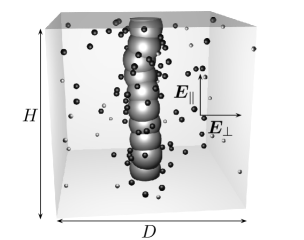
Figure 1: Simulation cell for a DNA segment with counterions (dark grey) and coions (light grey). Periodic boundary conditions are applied along the projected end-to-end distance $H$ of the DNA segment. The external electric field is applied either parallel ($\bm{E}_{||}$) or perpendicular ($\bm{E}_{\perp}$) to the PE axis.

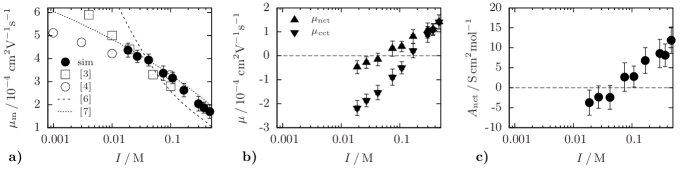
Figure 2: Hydrodynamic simulations of DNA in aqueous NaCl solution of various ionic strengths $I$ at $20\text{\,}\mathrm{\SIUnitSymbolCelsius}$. a) Electrophoretic DNA mobility $\mu_{\mathrm{m}}$ as obtained from simulations (filled symbols) and experiments (open symbols) as a function of $I$, compared to theories by Stigter Schellman and Stigter (1977) (dashed line) and Manning Manning (1981) (dotted line). b) Mobility of neutralizing counterions $\mu_{\mathrm{nct}}$, and condensed counterions $\mu_{\mathrm{cct}}$. c) Counterion excess conductivity $A_{\mathrm{nct}}$ according to Eq. (1).

In our hydrodynamic simulations we consider a PE consisting of charged beads together with neutralizing counterions and added symmetric salt, cf. Fig. 1. The vertical box height $H$ and lateral width $D$ are fluctuating while keeping the volume $HD^{2}$ and thus the concentration of monomers $c_{\mathrm{m}}$, neutralizing counterions $c_{\mathrm{nct}}$ and salt ion pairs $c_{\mathrm{s}}$ fixed. Periodic boundary conditions along the vertical axis are implemented by coupling the box height $H$ to the vertical PE extension. All particle positions $\bm{r}_{i}$ evolve according to the position Langevin equation, $\dot{\bm{r}}_{i}(t)=-\sum_{j}\bm{\mathrm{M}}_{ij}\cdot\nabla_{\bm{r}_{j}}U(t)+\bm{\xi}_{i}(t)$. The thermal coupling is modeled by a Gaussian white noise with $\left\langle\bm{\xi}_{i}(t)\right\rangle=\bm{0}$ and $\left\langle\bm{\xi}_{i}(t)\bm{\xi}_{j}(t^{\prime})\right\rangle=2\mathrm{k_{B}}T\,\bm{\mathrm{M}}_{ij}\delta(t-t^{\prime})$ according to the fluctuation-dissipation theorem. Hydrodynamic interactions are included via the Rotne-Prager-Yamakawa mobility tensor $\bm{\mathrm{M}}_{ij}$ Ermak and McCammon (1978), which accounts for finite hydrodynamic particle radii $a_{i}$ ($a_{i}=a_{\mathrm{m}},a_{\mathrm{ct}},a_{\mathrm{co}}$ for monomers, counterions, and coions). The interaction potential $U=U_{\mathrm{LJ}}+U_{\mathrm{C}}+U_{\mathrm{S}}+U_{\mathrm{ext}}$ consists of: i) A truncated, shifted Lennard-Jones potential, $U_{\mathrm{LJ}}/\mathrm{k_{B}}T=\epsilon\sum_{\langle ij\rangle}\left[(\sigma_{ij}/r_{ij})^{12}-2(\sigma_{ij}/r_{ij})^{6}+1\right]$ for $r_{ij}\leq\sigma_{ij}$ between ions and monomers that prevents electrostatic collapse of opposite charges, where $r_{ij}=|\bm{r}_{i}-\bm{r}_{j}|$ is the distance between particles $i$ and $j$ and $\sigma_{ij}=(a_{i}+a_{j})/2$ and $\epsilon$ define the soft-core distance and repulsion strength. ii) An unscreened Coulomb potential $U_{\mathrm{C}}/\mathrm{k_{B}}T=\ell_{\mathrm{B}}\sum_{\langle ij\rangle}q_{i}q_{j}/r_{ij}$, where $q_{i}$ denotes particle valency ($q_{i}=q_{\mathrm{m}},q_{\mathrm{ct}},q_{\mathrm{co}}$ for monomers, counterions, and coions) and $\ell_{\mathrm{B}}=\mathrm{e}^{2}/4\pi\epsilon_{\mathrm{r}}\epsilon_{0}\mathrm{k_{B}}T$ is the Bjerrum distance at which two unit charges interact with thermal energy $\mathrm{k_{B}}T$ ($\ell_{\mathrm{B}}=$7.21\text{\,}\mathrm{\SIUnitSymbolAngstrom}$$ in water at $20\text{\,}\mathrm{\SIUnitSymbolCelsius}$). iii) A harmonic potential, $U_{\mathrm{S}}/\mathrm{k_{B}}T=(K/2)\sum_{\langle ij\rangle}(r_{ij}-b)^{2}$, which acts between adjacent monomers only and ensures chain connectivity. iv) The external electric potential, $U_{\mathrm{ext}}/\mathrm{k_{B}}T=-\sum_{i}(q_{i}\mathrm{e}/\mathrm{k_{B}}T)\,\bm{E}\cdot\bm{r}_{i}$, with the electric field directed either parallel ($\bm{E}_{||}$) or perpendicular ($\bm{E}_{\perp}$) to the PE axis. Periodic boundary conditions along the PE axis are implemented by a one-dimensional resummation of the Coulomb interactions Naji and Netz (2006); the lateral and all hydrodynamic interactions are treated using the minimum image convention. Consequential finite-size effects are discussed in the supplementary information sup . The PE electrophoretic mobility $\mu_{\mathrm{m}}=\left\langle v_{\mathrm{m}}\right\rangle/E$ follows from the average monomer velocity along the E-field direction. In the absence of curvature, inter-chain and end effects (i.e. for high enough salt concentrations) and if orientation effects are negligible (i.e. for small E-fields), $\mu_{\mathrm{m}}$ follows from the parallel and perpendicular mobilities as $\mu_{\mathrm{m}}=(\mu_{\mathrm{m}}^{||}+2\mu_{\mathrm{m}}^{\perp})/3$. In the simulations we accordingly determine $\mu_{\mathrm{m}}^{||}$ and $\mu_{\mathrm{m}}^{\perp}$ separately by applying E-fields parallel and perpendicular to the PE axis and measuring the corresponding velocities. Possible non-linear effects have been carefully checked sup . The ionic strength includes contributions from the neutralizing counterions and is defined as $I=(c_{\mathrm{nct}}q_{\mathrm{ct}}^{2}+c_{\mathrm{s}}q_{\mathrm{ct}}^{2}+c_{\mathrm{s}}q_{\mathrm{co}}^{2})/2$.

In order to model DNA in aqueous NaCl solution at $20\text{\,}\mathrm{\SIUnitSymbolCelsius}$ we use Stokes radii of Na⁺ and Cl^- as $a_{\mathrm{ct}}=$1.84\text{\,}\mathrm{\SIUnitSymbolAngstrom}$$ and $a_{\mathrm{co}}=$1.29\text{\,}\mathrm{\SIUnitSymbolAngstrom}$$ as obtained from limiting conductivities Marcus (1997), an estimate of $a_{\mathrm{m}}=$10.47\text{\,}\mathrm{\SIUnitSymbolAngstrom}$$ for the DNA radius and valencies $q_{\mathrm{ct}}=1$, $q_{\mathrm{co}}=-1$ and $q_{\mathrm{m}}=-6$. The choice of monomer separation $b=a_{\mathrm{m}}$ ensures a linear charge density of $q_{\mathrm{m}}/b\simeq$0.57\text{\,}\mathrm{\SIUnitSymbolAngstrom}^{-1}$$. Although no bending rigidity is present in the model, the segment is sufficiently straight due to electrostatic repulsions, as appropriate for DNA (cf. Fig. 1). The simulation cell comprises $10$ DNA monomers, $60$ neutralizing counterions and $24$ salt pairs. The ionic strength is varied over the range $I=$19-468\text{\,}\mathrm{m}\mathrm{M}$$ by adjusting the cell width $D$. The field strengths applied are $E_{||}=$27.5\times 10^{6}\text{\,}\mathrm{V}\text{\,}{\mathrm{m}}^{-1}$$ and $E_{\perp}=$5.5\times 10^{6}\text{\,}\mathrm{V}\text{\,}{\mathrm{m}}^{-1}$$. We use $\epsilon=5$ for the LJ strength, $K/a_{\mathrm{ct}}^{2}=100$ for the bond stiffness, and $\eta=$1.003\times 10^{-3}\text{\,}\mathrm{Pa}\,\mathrm{s}$$ for the viscosity of water. The Langevin time-step is $0.06-0.12\text{\,}\mathrm{ps}$ and simulations are typically run for $0.3-4.1\text{\,}\mathrm{\SIUnitSymbolMicro s}$.

In Fig. 2a we plot the DNA electrophoretic mobility $\mu_{\mathrm{m}}$ as a function of the ionic strength, $I$, together with experimental data for long DNA from Refs. Hartford and Flygare (1975); Hoagland et al. (1999). Noting that there are no free fitting parameters and given the substantial scatter in the experimental data, we conclude that our coarse-grained DNA model is quite accurate. The mobility $\mu_{\mathrm{m}}$ decreases with increasing $I$ which will be rationalized in terms of hydrodynamic screening effects below. We additionally show theoretical results from Stigter Schellman and Stigter (1977) and Manning Manning (1981).

Theoretically, only little attention has been paid to E-field-induced counterion dynamics in PE solutions. In this context the phenomenon of counterion condensation at highly charged PEs that are characterized by a Manning parameter $\xi_{\mathrm{M}}=|q_{\mathrm{ct}}q_{\mathrm{m}}\ell_{\mathrm{B}}/b|>1$ has to be taken into account. For highly charged PEs such as DNA ($\xi_{\mathrm{M}}=4.17$) electrostatic attraction of counterions towards the PE overcomes entropic repulsion giving rise to increased accumulation of counterions in the very vicinity of the PE Manning (1969); Naji and Netz (2006). In particular, the assumption that condensed counterions stick to the PE Schellman and Stigter (1977); Manning (1981) has not been scrutinized, despite experimental evidence that condensed counterions are not immobilized on the PE surface Nagasawa et al. (1972). In Fig. 2b we show the electrophoretic mobility of two counterion ensembles, first condensed counterions within a distance $r^{\ast}_{\perp}=a_{\mathrm{m}}+4a_{\mathrm{ct}}=$17.8\text{\,}\mathrm{\SIUnitSymbolAngstrom}$$ from the DNA axis ($\mu_{\mathrm{cct}}$) and secondly the set of counterions closest to the DNA axis that neutralize the DNA charge ($\mu_{\mathrm{nct}}$). At low ionic strength the hydrodynamic drag exerted by the DNA on the counterions exceeds the external electric force and the mobility for both sets is negative, i.e. the counterions are dragged along by the PE. At high ionic strength the hydrodynamic interactions are sufficiently screened so that the electric field dominates and the counterions move opposite to the DNA. In fact, a salt and PE charge density dependent sign reversal of the electrophoretic counterion mobility has been inferred from transference experiments some time ago Nagasawa et al. (1972). Direct measurements of counterion electrophoretic mobilities can in principle be performed with pulsed field gradient NMR Böhme and Scheler (2004).

We define the excess contribution of the counterions to the conductivity of a PE solution as

$$A_{\mathrm{nct}}=(\sigma-q_{\mathrm{m}}\mathrm{e}c_{\mathrm{m}}\mu_{\mathrm{m}}-\sigma_{\mathrm{s}}^{0})/c_{\mathrm{nct}}$$ (1)

where $\sigma$ and $\sigma_{\mathrm{s}}^{0}$ denote the specific conductivities of the salt solution with and without the PE chain, respectively. In our simulations, $\sigma$ results from the separate electrophoretic contributions as $\sigma/\mathrm{e}=q_{\mathrm{ct}}c_{\mathrm{nct}}\mu_{\mathrm{nct}}-q_{\mathrm{m}}c_{\mathrm{m}}\mu_{\mathrm{m}}+q_{\mathrm{ct}}c_{\mathrm{s}}\mu_{\mathrm{ct}}-q_{\mathrm{co}}c_{\mathrm{s}}\mu_{\mathrm{co}}$, while the pure electrolyte conductivity $\sigma_{0}$ is obtained from separate simulations as $\sigma_{\mathrm{s}}^{0}=q_{\mathrm{ct}}c_{\mathrm{s}}\mu_{\mathrm{ct}}^{0}-q_{\mathrm{co}}c_{\mathrm{s}}\mu_{\mathrm{co}}^{0}$. As seen in Fig. 2c, the counterion excess conductivity $A_{\mathrm{nct}}$ increases with increasing salt concentration and changes sign, and thus directly reflects the salt-dependent counterion mobility anomaly for the experimentally easily accessible conductivity.

To gain further insight, we now shift to weakly charged PEs (Manning parameter $\xi_{\mathrm{M}}<1$), where the ion distribution around a PE is correctly described by linear Debye-Hückel (DH) theory and the electrophoretic mobilities of PE and ions can be constructed using Green’s functions Barrat and Joanny (1996). The DH ionic charge distribution around a sphere of radius $a$ and surface charge density $q\mathrm{e}/4\pi a^{2}$ is for $\kappa a<1$ given by $n(r)=-q\mathrm{e}\kappa^{2}\mathrm{e}^{-\kappa(r-a)}/[4\pi r(1+\kappa a)]$, where $\kappa^{-1}=(8\pi\ell_{\mathrm{B}}I)^{-1/2}$ is the DH screening length. On the Stokes level, the solvent flow field $\bm{u}$ induced by an external electric field $\bm{E}$ acting on the ionic charge distribution $n(r)$ is $\bm{u}(\bm{r})=\bm{G}(\bm{r})\,q\mathrm{e}\bm{E}$, where the screened hydrodynamic Green’s function $G_{\alpha\beta}(\bm{r})$ reads sup

$$G_{\alpha\beta}(\bm{r})=A\bigg{(}\delta_{\alpha\beta}-3\frac{x_{\alpha}x_{\beta}}{r^{2}}\bigg{)}+2B\frac{x_{\alpha}x_{\beta}}{r^{2}},$$ (2)

where $\alpha,\beta=x,y,z$ and $B=\mathrm{e}^{-\kappa(r-a)}/[4\pi\eta r(1+\kappa a)]$ and $A=B\,[1+\kappa r+\kappa^{2}r^{2}-\mathrm{e}^{\kappa(r-a)}(1+\kappa a+\kappa^{2}a^{2}/3)]/(\kappa^{2}r^{2})$. In the limit of zero salt $\kappa\to 0$, the Stokes solution for a translating sphere is recovered Kim and Karrila (2005). For vanishing radius $a\to 0$, Eq. (2) reduces to a previously derived expression Long and Ajdari (2001). Noting that Eq. (2) fulfills the no-slip condition on the sphere’s surface, its electrophoretic mobility follows from $\mu_{\mathrm{s}}=q\mathrm{e}\,G_{xx}(r=a)$ as

$$\frac{\mu_{\mathrm{s}}}{q\mathrm{e}\mu_{0}}=\frac{1}{1+\kappa a}\,,$$ (3)

which is the classical result derived by Debye and Hückel Kim and Karrila (2005). Here $\mu_{0}=1/6\pi\eta a$ is the Stokes mobility.

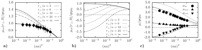
Figure 3: Results for a weakly charged PE with Manning parameter $\xi_{\mathrm{M}}=|q_{\mathrm{ct}}q_{\mathrm{m}}\ell_{\mathrm{B}}/b|=0.4$. a) Coion mobility $\mu_{\mathrm{co}}(r_{\perp},0)$ for various fixed distances $r_{\perp}$ from the PE as a function of $(\kappa a)^{2}$. The hydrodynamic drag exerted by the PE on the coions increases their mobility as compared to the case without PE, Eq. (3) ($r_{\perp}/a\to\infty$, solid line). The latter compares well with hydrodynamic simulations of a simple salt solution (filled symbols). b) Counterion mobility $\mu_{\mathrm{ct}}(r_{\perp},0)$ at distance $r_{\perp}$ from the PE which exhibits a sign change. For small $r_{\perp}$ and low salt, counterions are dragged along with the PE ($\mu_{\mathrm{ct}}(r_{\perp},0)<0$). c) Comparison of theoretical predictions (solid lines) and hydrodynamic simulations (filled symbols) for the PE mobility $\mu_{\mathrm{m}}$, neutralizing counterion mobility $\mu_{\mathrm{nct}}$ and condensed counterion mobility $\mu_{\mathrm{cct}}$. The condensed counterion mobility changes sign. We also show the parallel and perpendicular PE mobilities $\mu_{\mathrm{m}}^{\parallel}$ (dotted line) and $\mu_{\mathrm{m}}^{\perp}$ (short dashed line).

To leading order in $a/r$ the electrophoretic coupling matrix $\mu_{\mathrm{ss}}^{\alpha\beta}(\bm{r})$ ($\alpha,\beta=x,y,z$) between two charged spheres is obtained via a multipole expansion Kim and Karrila (2005) as

$$\mu_{\mathrm{ss}}^{\alpha\beta}(\bm{r})=q\mathrm{e}\left(1+\frac{a^{2}}{6}\,\nabla^{2}_{\bm{r}}\right)G_{\alpha\beta}(\bm{r})\,.$$ (4)

Approximating the PE as a straight chain of charged spheres at spacing $b$ oriented along the $z$-axis, the PE mobilities follow by superposition as $\mu_{\mathrm{m}}^{\perp}=\mu_{\mathrm{s}}+2\sum_{j=1}^{\infty}\mu_{\mathrm{ss}}^{xx}(r_{\perp}=0,bj)$ and $\mu_{\mathrm{m}}^{\parallel}=\mu_{\mathrm{s}}+2\sum_{j=1}^{\infty}\mu_{\mathrm{ss}}^{zz}(r_{\perp}=0,bj)$. Here $r_{\perp}$ denotes the lateral distance from the PE axis. For the orientationally averaged mobility $\mu_{\mathrm{m}}=(\mu_{\mathrm{m}}^{\parallel}+2\mu_{\mathrm{m}}^{\perp})/3$, we obtain the closed-form expression

$$\frac{\mu_{\mathrm{m}}}{q\mathrm{e}\mu_{0}}=\frac{\mu_{\mathrm{s}}}{q\mathrm{e}\mu_{0}}-\frac{a(6+\kappa^{2}a^{2})}{3b(1+\kappa a)}\,\mathrm{e}^{\kappa a}\,\ln\left(1-\mathrm{e}^{-\kappa b}\right)\,.$$ (5)

In the limit of low screening, $\kappa a\to 0$, Eq. (5) decays logarithmically with increasing ionic strength as $\mu_{\mathrm{m}}/q\mathrm{e}\mu_{0}=-2(a/b)\ln(\kappa b)$, in accord with previous results for weakly charged PEs Barrat and Joanny (1996); Manning (1981). In the same fashion the perpendicular and parallel distance-dependent ion mobilities follow as $\mu_{\mathrm{co/ct}}^{\perp}(r_{\perp},z)=\mu_{\mathrm{s}}\pm\sum_{j=-\infty}^{+\infty}\mu_{\mathrm{ss}}^{xx}(r_{\perp},z+bj)$ and $\mu_{\mathrm{co/ct}}^{\parallel}(r_{\perp},z)=\mu_{\mathrm{s}}\pm\sum_{j=-\infty}^{+\infty}\mu_{\mathrm{ss}}^{zz}(r_{\perp},z+bj)$, respectively; the plus/minus sign applies to coions/counterions.

In Fig. 3 we compare the foregoing theoretically predicted electrophoretic mobilities of monomers and ions (obtained by summing over contributions from $23$ spheres) to the hydrodynamic simulations of a weakly charged PE with Manning parameter $\xi_{\mathrm{M}}=0.4$ in a field of strength $aq\mathrm{e}E/\mathrm{k_{B}}T=0.2$. The simulation cell comprises 24 PE monomers, 24 neutralizing counterions and 24 salt pairs with equal radii $a_{\mathrm{m}}=a_{\mathrm{co}}=a_{\mathrm{ct}}\equiv a$, valencies $q_{\mathrm{m}}=q_{\mathrm{co}}=-q_{\mathrm{ct}}\equiv q$ and monomer spacing $b=2a$. For intrinsically flexible PEs, the straight PE conformation in our simulations and theory is realistic only for low enough salt concentration as long as the effective persistence length is larger than the screening length. In Fig. 3a,b we show the orientationally averaged coion and counterion mobilities $\mu_{\mathrm{co/ct}}(r_{\perp},0)=[2\mu_{\mathrm{co/ct}}^{\perp}(r_{\perp},0)+\mu_{\mathrm{co/ct}}^{\parallel}(r_{\perp},0)]/3$ for fixed vertical coordinate $z=0$ and various fixed distances $r_{\perp}$ from the PE as a function of the rescaled salt concentration $(\kappa a)^{2}\sim c_{\mathrm{s}}$. The mobilities of coions are increased and those of counterions are decreased by the presence of the PE. This entraining effect is larger for smaller salt concentration and smaller $r_{\perp}$. The ion mobilities for $r_{\perp}=\infty$ reflect pure electrolyte friction effects and in Fig. 3a compare very well with simulation results for a simple salt solution. In Fig. 3c we compare analytical predictions for the PE mobility $\mu_{\mathrm{m}}$, the neutralizing counterion mobility $\mu_{\mathrm{nct}}$, and the condensed counterion mobility $\mu_{\mathrm{cct}}$ (obtained from counterions within a shell of $r_{\perp}^{\ast}=5a$ around the PE) with the simulations. Here $\mu_{\mathrm{nct}}$ and $\mu_{\mathrm{cct}}$ are obtained from $\mu_{\mathrm{ct}}(r_{\perp},0)$ by spatially averaging over the DH counterion distribution around a straight chain of charged spheres at fixed vertical coordinate $z=0$. With increasing salt concentration, $\mu_{\mathrm{cct}}$ changes its sign, similar to the DNA results (cf. Fig. 2b). This shows that the salt-induced counterion mobility anomaly is not restricted to the non-linear regime and is fully explained by screening effects of the hydrodynamic coupling tensor.

Our simulation method neglects local solvation and DNA structural effects. The good agreement between experimental and simulation results could imply that those effects are of minor importance for the electrokinetic behavior. Nevertheless, an extension of the model to more realistic charge distributions is planned. Likewise, the analytic Green’s function approach will be generalized to include relaxation effects in addition to retardation.