Hybrid elastic/discrete-particle approach to biomembrane dynamics with application to the mobility of curved integral membrane proteins

Abstract

We introduce a simulation strategy to consistently couple continuum biomembrane dynamics to the motion of discrete biological macromolecules residing within or on the membrane. The methodology is used to study the diffusion of integral membrane proteins that impart a curvature on the bilayer surrounding them. Such proteins exhibit a substantial reduction in diffusion coefficient relative to “flat” proteins; this effect is explained by elementary hydrodynamic considerations.

Lipid-bilayer membranes are among the most important and most versatile components of biological cells textbook ; gennis ; biomembranes protect cells from their surroundings, provide a means to compartmentalize subcellular structures (and the functions of these structures) and act as a scaffolding for countless biochemical reactions involving membrane associated proteins. Our conceptual picture of biological membranes as a “two-dimensional oriented solution of integral proteins … in the viscous phospholipid bilayer”singer was popularized well over thirty years ago. Quantitative physical models for the energetics helfrich and dynamics Brochard associated with shape fluctuations of homogeneous fluid membranes and for the lateral diffusion coefficient of integral membrane proteins within a flat bilayer Saffmann were developed shortly thereafter and still find widespread use up to this day.

Interestingly, the coupling of protein diffusion to the shape of the membrane surface has become a subject of study only relatively recently (see Halle_NMR ; Seifert_pre ; Naji and references within). One well studied consequence of membrane shape fluctuations is that a protein must travel a longer distance between two points in 3D space if the paths connecting these points are constrained to lie on a rough surface as opposed to a flat plane. This purely geometric effect is expected to have practical experimental implications; measurements that capture a 2D projection of the true motion over the membrane surface will infer diffusion coefficients of diminished magnitude relative to the intrinsic lateral diffusion locally tangent to the bilayer surface Halle_NMR ; Seifert ; Gov_pre ; Seifert_pre ; Naji . Beyond this generic effect, which should apply to anything moving on the membrane surface in relatively passive fashion (lipids, proteins, choleseterol, etc.), certain membrane associated proteins effect shape changes in the bilayer. Specific examples include the SERC1a calcium pump serc1a and BAR (Bin, Amphiphysin, Rvs) domain dimers bar_science . Direct structural evidence from X-ray crystallography serc1a ; bar_science , experimental studies of vesicle topology at the micron scale Girard ; bar_science , and atomically detailed simulations voth all indicate the ability of these proteins to drive membrane curvature (see Fig. 1).

The diffusion of membrane proteins with intrinsic curvature is more complex than the diffusion of a relatively passive spectator and remains incompletely explored in the literature. Although stochastic differential equations coupling the lateral motion of curved proteins to thermal shape fluctuations of a continuous elastic bilayer have been proposed Seifert ; Seifert_crv , these equations have only been analyzed under the simplifying assumption that the protein does not affect the shape of the membrane surface. Under such an approximation, it was predicted both analytically Seifert and numerically Seifert_crv that curved proteins are expected to diffuse more rapidly than flat ones. The full numerical analysis provided in the present work suggests exactly the opposite effect–protein curvature decreases lateral mobility across the bilayer. The disagreement with previous work is attributable to the fact that the protein’s influence on bilayer shape is of primary importance (see Fig. 1) and cannot be ignored.

Our starting point is the Monge-gauge Helfrich Hamiltonian helfrich for energetics of a homogeneous membrane surface under conditions of vanishing tension

$${\mathcal{H}}_{0}=\frac{1}{2}\int_{{\mathcal{A}}_{\bot}}\!{\mathrm{d}}{\mathbf{x}}\,\big{[}K_{\mathrm{m}}\,(\nabla^{2}h)^{2}+2K^{\prime}_{\mathrm{m}}\,{\mathcal{G}}(h)\big{]},$$ (1)

where $h({\mathbf{x}})\equiv h(x,y)$ describes the local membrane displacement from a flat reference plane at $z=0$ (see Fig. 1). Here, ${\mathcal{G}}(h)=(\partial_{xx}h\partial_{yy}h-\partial_{xy}h\partial_{xy}h)$ is the Gaussian curvature and $K_{\mathrm{m}}$ and $K^{\prime}_{\mathrm{m}}$ are the membrane bending modulus and saddle-splay modulus, respectively. The integration region, ${\mathcal{A}}_{\bot}=L^{2}$, is always taken to be a square box with periodic boundary conditions assumed. We treat membrane proteins as localized regions of enhanced rigidity within the bilayer. A single protein centered within the bilayer at position $({\mathbf{r}}(t),h({\mathbf{r}}(t)))\equiv(x(t),y(t),h(x(t),y(t)))$ is thus assumed to modify the Hamiltonian as ${\mathcal{H}}={\mathcal{H}}_{0}+{\mathcal{H}}_{\mathrm{int}}$ with

$${\mathcal{H}}_{\mathrm{int}} = \frac{1}{2}\int_{{\mathcal{A}}_{\bot}}\!\!\!{\mathrm{d}}{\mathbf{x}}\,G_{\mathrm{p}}({\mathbf{x}}-{\mathbf{r}}(t))\,\big{[}K_{\mathrm{p}}\,(\nabla^{2}h-2C_{\mathrm{p}})^{2}$$

$$\qquad\qquad\qquad-K_{m}\,(\nabla^{2}h)^{2}+2(K^{\prime}_{\mathrm{p}}-K^{\prime}_{\mathrm{m}})\,{\mathcal{G}}(h)\big{]}.$$

$K_{\mathrm{p}}$ and $K^{\prime}_{\mathrm{p}}$ are the protein bending and saddle-splay moduli and $C_{\mathrm{p}}$ is the spontaneous curvature associated with protein shape. The protein shape function $G_{\mathrm{p}}({\mathbf{x}}-{\mathbf{r}}(t))$ describes the envelope of protein influence over bilayer elastic properties; the specific function chosen will be discussed in detail below.

Using a Fourier representation $h({\mathbf{x}})=\frac{1}{L^{2}}\sum_{{\mathbf{q}}}h_{{\mathbf{q}}}\,e^{{\mathrm{i}}{\mathbf{q}}\cdot{\mathbf{x}}}$, membrane dynamics may be cast as a set of coupled Langevin equations for the individual Fourier modes Granek ; Brown_prl

$$\dot{h}_{{\mathbf{q}}}(t)=\Lambda_{\mathbf{q}}F_{{\mathbf{q}}}(t)+\sqrt{k_{\mathrm{B}}TL^{2}\Lambda_{{\mathbf{q}}}}\,\,\xi_{{\mathbf{q}}}(t),$$ (3)

where $F_{{\mathbf{q}}}(t)$ is the Fourier-transform of the force per unit area $F({\mathbf{x}},t)=-\delta{\mathcal{H}}/\delta h({\mathbf{x}},t)$, $\Lambda_{{\mathbf{q}}}=1/(4\eta\,q)$ corresponds to the Oseen hydrodynamic kernel $\Lambda({\mathbf{x}})=1/(8\pi\eta|{\mathbf{x}}|)$, and $\xi_{{\mathbf{q}}}(t)$ is a Gaussian white noise with $\langle\xi_{{\mathbf{q}}}(t)\rangle=0$ and $\langle\xi_{{\mathbf{q}}}(t)\,\xi_{{\mathbf{q}^{\prime}}}(t^{\prime})\rangle=2\delta_{{\mathbf{q}},-{\mathbf{q}}^{\prime}}\,\delta(t-t^{\prime})$, to ensure satisfaction of the fluctuation-dissipation theorem.

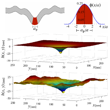
Figure 1: (Color online) An appropriately shaped protein will tend to distort the local shape of the bilayer into a bent configuration. In our simulations, the protein’s effective size is defined via the envelope function in Eq. (5) (displayed next to the cartoon, top). The distortion is most readily seen by minimizing $\mathcal{H}$ for the composite protein-bilayer system (middle), however the protein’s influence is strong enough to maintain visibly apparent perturbations, even in the presence of fluctuations (bottom). See Table 1 for parameters.

The protein’s position may similarly be described in terms of a Langevin equation that implicitly enforces protein localization to the membrane surface Naji ; Seifert_pre . The two independent variables describing this motion are the components of ${\mathbf{r}}(t)$ (with $i,j=1,2$ and summation convention assumed)

$$\dot{r}_{i}(t)=D_{0}\,v_{i}+\sqrt{2D_{0}}\,\tau_{ij}\,\eta_{j}(t)+\frac{D_{0}}{k_{\mathrm{B}}T}(g^{-1})_{ij}f_{j}.$$ (4)

Here $(g^{-1})_{ij}=\delta_{ij}-\partial_{i}h\,\partial_{j}h/g$ is the inverse metric tensor, $g=1+(\nabla h)^{2}$ is the determinant of the metric $g_{ij}=\delta_{ij}+\partial_{i}h\,\partial_{j}h$ and we have defined $\partial_{i}\equiv\partial/\partial x_{i}$. Equation (4) introduces geometric factors including $v_{i}=-\big{[}(g^{-1})_{jk}\,\partial_{j}\partial_{k}h\big{]}\,\partial_{i}h/{g}$ and $\tau_{ij}=\delta_{ij}-\partial_{i}h\,\partial_{j}h/(g+\sqrt{g})$ (i.e., the square-root of the inverse metric tensor $(g^{-1})_{ij}=\tau_{ik}\,\tau_{jk}$). The Gaussian white-noise $\eta_{i}(t)$ with $\langle\eta_{i}(t)\rangle=0$ and $\langle\eta_{i}(t)\,\eta_{j}(t^{\prime})\rangle=\delta_{ij}\,\delta(t-t^{\prime})$ guarantees that a tracer particle (defined by $\mathcal{H}_{\mathrm{int}}=0$) undergoes a curvilinear random walk over the membrane surface with diffusion coefficient $D_{0}$. The last term in Eq. (4) reflects the effect of the interaction-induced force $f_{i}=-\partial{\mathcal{H}}_{\mathrm{int}}/\partial x_{i}$.

Equations (1)-(4) specify the stochastic thermal evolution for a single curved protein coupled to an elastic membrane. As noted above, equations very similar to these have been proposed previously Seifert ; Seifert_crv , but have only been analyzed by neglecting the contribution of $\mathcal{H}_{\mathrm{int}}$ to $F_{\mathbf{q}}$ while maintaining its contribution to $f_{i}$. To avoid this uncontrolled approximation, it is necessary to introduce a numerical algorithm that can consistently couple protein position ${\mathbf{r}}(t)$ to membrane undulations $h({\mathbf{x}},t)$.

parameter	box	lattice		protein	temperature	bare protein	bilayer	protein	saddle-splay	protein	solvent
	dimension	spacing		area		diffusion	bending	bending	moduli	spontaneous	viscosity
						coefficient	modulus	modulus		curvature
symbol	$L$	$a$	$M=\frac{L}{a}$	$A_{\mathrm{p}}$	$T$	$D_{0}$	$K_{\mathrm{m}}$	$K_{\mathrm{p}}$	$K^{\prime}_{\mathrm{m(p)}}$	$C_{\mathrm{p}}$	$\eta$
value	250nm	2.5nm	100	100${\mathrm{nm}}^{2}$	300${\mathrm{K}}$	5.0$\frac{\mu{\mathrm{m}}^{2}}{{\mathrm{s}}}$	5$k_{\mathrm{B}}T$	40$k_{\mathrm{B}}T$	$-K_{\mathrm{m(p)}}$	0.1${\mathrm{nm}}^{-1}$	$\eta_{\mathrm{w}}$=0.001${\mathrm{Pa}}\cdot{\mathrm{s}}$

Table 1: Default parameter values used in the simulations. The protein area is chosen as $A_{\mathrm{p}}=(4a)^{2}$ (giving a protein diameter of $a_{\mathrm{p}}\sim 10$nm), the $D_{0}$ value qualitatively reflects the motion of band 3 protein dimers on the surface of human red blood cells Brown_prl , and $\eta_{\mathrm{w}}$ stands for the viscosity of water. For simplicity we assume that both bilayer and protein saddle-splay moduli are equal in magnitude but opposite in sign to the corresponding bending moduli.

For both physical and numerical purposes, we must truncate the membrane modes at some short-distance scale $a$, which can for example be taken to represent the typical molecular (lipid) size or bilayer thickness. We thus limit the Fourier modes appearing in Eq. (3) to ${\mathbf{q}}=(q_{x},q_{y})=(2\pi n,2\pi m)/L$ where $M=L/a$ with integer $n,m$ in the range $-M/2<n,m\leq M/2$. In principle, this reduced set of modes describes a fully continuous membrane height profile via $h({\mathbf{x}})=\frac{1}{L^{2}}\sum_{{\mathbf{q}}}h_{{\mathbf{q}}}\,e^{{\mathrm{i}}{\mathbf{q}}\cdot{\mathbf{x}}}$ at any given point ${\mathbf{x}}$. However, it is computationally advantageous to explicitly track the membrane height only over the discrete $M\times M$ real-space lattice (defined at positions ${\mathbf{x}}_{\alpha}=(p,q)a$ with integer $0\leq p,q<M$) conjugate to the chosen $h_{{\mathbf{q}}}$’s via Fast-Fourier Transformation FFTW .

The interaction between a fully continuous variable describing protein position ${\mathbf{r}}(t)$ and a discrete representation of the membrane height field $\{h({\mathbf{x}}_{\alpha},t)\}$ poses certain challenges. A minor issue is that Eq. (4) requires the shape of the membrane surface over the entire $x,y$ plane and not just at the lattice sites $\{{\mathbf{x}}_{\alpha}\}$. This problem is readily handled via linear interpolation to obtain $h({\mathbf{x}},t)$ and the required derivatives at arbitrary ${\mathbf{x}}$ from the corresponding neighboring lattice values Seifert_pre . A more complex problem involves the dynamics of the $h_{\mathbf{q}}(t)$’s in Eq. (3). The forces in this equation include contributions due to the coupling between protein and bilayer from Eq. (Hybrid elastic/discrete-particle approach to biomembrane dynamics with application to the mobility of curved integral membrane proteins). The envelope function $G_{\mathrm{p}}({\mathbf{x}})$ reflects protein size and is quite localized in real space; the natural way to deal with Eq. (Hybrid elastic/discrete-particle approach to biomembrane dynamics with application to the mobility of curved integral membrane proteins) (and the related force expressions) is to approximate the integral by simple quadrature, i.e. $\int{\mathrm{d}}{\mathbf{x}}\,G_{\mathrm{p}}({\mathbf{x}}-{\mathbf{r}}(t))\mathcal{F}({\mathbf{x}})\approx a^{2}\sum_{\alpha}G_{\mathrm{p}}({\mathbf{x}}_{\alpha}-{\mathbf{r}}(t))\mathcal{F}({\mathbf{x}}_{\alpha})$ for arbitrary function $\mathcal{F}$. To define a numerical scheme that is both efficient and accurate, the specific functional form chosen for $G_{\mathrm{p}}$ is critical. Naive continuous choices like 2D Gaussians Brown_prl ; Seifert_crv lead to an effective normalization (as computed by quadrature) that varies with the offset between the envelope center and the discrete lattice. Piecewise linear forms for $G_{\mathrm{p}}$ can be defined that suffer no such normalization issue, but such functions lead to discontinuous derivatives as the protein-lattice offset changes. Both scenarios are unacceptable as these numerical issues lead to a breaking of the homogeneity of the membrane surface; the protein will tend to favor (or disfavor) lattice sites over other regions of space.

Our numerical description of coupled membrane-protein dynamics shares features with the Immersed Boundary formulation of hydrodynamics peskin . In that work, a series of envelope functions are introduced that are continuous, localized in space and strictly preserve normalization as evaluated by quadrature. For our purposes, we take $G_{\mathrm{p}}({\mathbf{x}})=(A_{\mathrm{p}}/a^{2})\phi(x/a)\,\phi(y/a)$ with peskin

$$\phi\big{(}2u\big{)}=\frac{1}{16}\left\{\begin{array}[]{lc}5+2u-\sqrt{-7-12u-4u^{2}}&{-2\leq u\leq-1,}\\ 3+2u+\sqrt{1-4u-4u^{2}}&{-1\leq u\leq 0,}\\ 3-2u+\sqrt{1+4u-4u^{2}}&{0\leq u\leq 1,}\\ 5-2u-\sqrt{-7+12u-4u^{2}}&{1\leq u\leq 2,}\end{array}\right.$$ (5)

and zero for all other $u$ values (see Fig. 1 for a plot). $A_{\mathrm{p}}$ defines an effective protein area and the envelope function is non-vanishing over a total of 64 lattice sites. In order to simulate the dynamics of the system, we evolve Eqs. (3) and (4) in time via the Euler-Maruyuma method maru . The resulting algorithm is essentially an application of “Brownian dynamics with hydrodynamic interactions” mccammon applied to membrane shape fluctuations and protein motion. Adopting the envelope function defined in Eq. (5) allows a seamless melding of the approaches introduced in Refs. Naji ; Seifert_pre ; Brown_prl (a detailed description of our algorithm will be provided in a future publication).

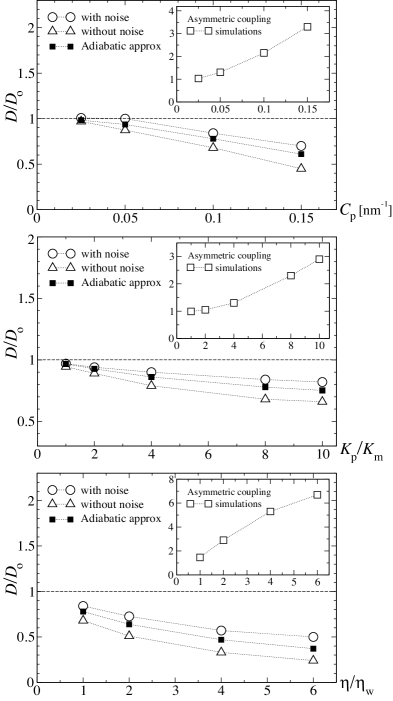
Figure 2: Projected diffusion coefficients for protein motion on an elastic membrane. In each panel, one of the three parameters $K_{\mathrm{p}}$ (protein bending modulus), $C_{\mathrm{p}}$ (protein spontaneous curvature), and $\eta$ (medium viscosity) is varied as indicated while holding the remaining physical properties at the default values indicated in Table 1. Circles indicate the results of full simulations including thermal motion of both the bilayer and the protein. The triangles indicate results obtained by turning off all bilayer shape fluctuations (i.e. setting $T=0$ for membrane undulations modes) and the solid squares indicate the results of the adiabatic theory discussed in the text. Insets show simulation results obtained within the asymmetric coupling approximation. Errorbars are approximately the size of the symbols. Diffusion coefficients are calculated as $D=\overline{[{\mathbf{r}}(t)-{\mathbf{r}}(0)]^{2}}/(4t)$. The simulations run for $\sim 5\times 10^{7}$ time steps of size $\Delta t\sim 0.01$ns, ensuring both numerical accuracy and statistically reliable results. The protein’s root-mean-square displacements over the course of the simulations are approximately 100nm (i.e. 20 times the protein’s radius).

The protein’s influence on the membrane is most easily seen in the absence of thermal shape fluctuations of the membrane, but for sufficiently large $C_{\mathrm{p}}$ and $K_{\mathrm{p}}$ values the effect of the protein remains clearly visible despite thermal fluctuations of the membrane surface (see Fig. 1). The average distortion of the membrane surrounding the protein is sufficient to significantly slow protein motion in all cases we have studied (see Fig. 2). This slowing derives from two effects. First, the protein tends to trap itself in the deformation created by its own perturbation to the bilayer. The energy-minimized configuration displayed in Fig. 1 places the protein at the bottom of a curved valley; attempted diffusion up the walls of this valley is hindered by the interaction-induced force in Eq. (4). Second, $x,y$ translation of the protein is accompanied by translation of the membrane deformation surrounding this protein. The hydrodynamic effects included in Eq. (3) dictate that the translation of such a deformation is resisted by the viscous drag of the medium surrounding the bilayer. This drag acts in addition to the usual quasi-2D drag incorporated within $D_{0}$ and slows protein motion. These effects are most pronounced when shape fluctuations of the bilayer are neglected by setting $T=0$ in Eq. (3). Increasing the local deformation around the protein or the solvent viscosity both decrease $D$. In Fig. 2 we display three means to control this effect. Increasing $C_{\mathrm{p}}$ drives large deformations from a flat plane for any finite $K_{\mathrm{p}}$. Larger values of $K_{\mathrm{p}}$ will tend to increase this effect up until the point where the rigidity of the protein becomes effectively infinite and the response to the protein saturates. The hydrodynamic drag in our model is controlled via $\eta$; increases in $\eta$ reduce $D$ as effectively as do perturbations to membrane shape.

Within the asymmetric coupling approximation, which ignores the influence of the protein on membrane shape, it is predicted that bilayer shape fluctuations will enhance curved protein mobility Seifert ; Seifert_crv (i.e. $D>D_{0}$, insets Fig. 2). Although this effect can be seen in our simulations, the enhancement is slight (relative to the similar effect within the aforementioned approximation scheme) and can not overcome the dominant slowing caused by the protein’s distortion of the bilayer (compare open circles and triangles, Fig. 2). We find $D<D_{0}$ for all cases studied, which represents a qualitative departure from earlier predictions.

We may approximately account for the viscous drag effect discussed above by invoking an adiabatic approximation and assuming that the energy-minimized membrane distortion profile (denoted by $\bar{h}({\mathbf{x}},t)$) instantaneously tracks protein position. Hence,

$$\dot{\bar{h}}({\mathbf{x}},t)=-{\mathbf{v}}\cdot\nabla\bar{h}({\mathbf{x}},t),$$ (6)

for a protein moving at constant lateral velocity ${\mathbf{v}}$. The power dissipated by viscous losses in the medium may be calculated from $P=\frac{1}{L^{2}}\sum_{{\mathbf{q}}}\dot{\bar{h}}_{{\mathbf{q}}}(t)F_{-{\mathbf{q}}}(t)$, where $F_{{\mathbf{q}}}(t)$ follows from Eq. (3) as $F_{{\mathbf{q}}}=\dot{\bar{h}}_{{\mathbf{q}}}/\Lambda_{{\mathbf{q}}}$. Thus, by using Eq. (6), the power loss may be written as $P=\frac{1}{L^{2}}\sum_{{\mathbf{q}}}({\mathbf{v}}\cdot{\mathbf{q}})^{2}|\bar{h}_{{\mathbf{q}}}|^{2}/\Lambda_{{\mathbf{q}}}\equiv|{\mathbf{v}}|^{2}/\mu_{\mathrm{def}}$ with $\mu_{\mathrm{def}}$ being the effective mobility of the deformation. The effective protein diffusion coefficient follows from $D_{\mathrm{def}}=\mu_{\mathrm{def}}k_{\mathrm{B}}T$ and $D^{-1}=(D_{0}^{-1}+D_{\mathrm{def}}^{-1})$ to give

$$\frac{1}{D}\approx\frac{1}{D_{0}}+\frac{2\eta}{k_{\mathrm{B}}TL^{2}}\sum_{{\mathbf{q}}}|{{\mathbf{q}}}|^{3}|\bar{h}_{{\mathbf{q}}}|^{2}.$$ (7)

This expression depends only on the minimized deformation profile of the membrane at fixed protein position and is readily calculated (shown as solid squares in Fig. 2). Although the approximation is imperfect due to neglect of membrane fluctuations and the self-trapping effect discussed above, the adiabatic results serve as a reliable estimator of the observed trends for the full simulation.

We are not aware of experimental studies that specifically investigate the role of protein curvature on self-diffusion, but do note that recent experiments urbach show deviations from the standard theory Saffmann used to predict membrane-protein mobility. The effect described here may prove to be important in describing these deviations for certain proteins. The solvent viscosity dependence we find is at odds with the weak (logarithmic) dependence expected for flat proteins Saffmann and provides a concrete means to verify our predictions experimentally.

This work is supported by the NSF (CHE-034916, CHE-0848809, DMS-0635535), the BSF (2006285) and the Camille and Henry Dreyfus Foundation. We thank N. Gov, H. Diamant and H. Boroudjerdi for helpful discussions.

References

- (1) B. Alberts et al., Molecular Biology of the Cell (Galland, New York, 2002)
- (2) R.B. Gennis, Biomembranes: Molecular Structure and Function. (Springer-Verlag, Berlin, 1989)
- (3) S.J. Singer, G.L. Nicolson, Science 175, 720 (1972)
- (4) W. Helfrich, Z. Naturforsch 28c, 693 (1973)
- (5) F. Brochard, J. F. Lennon, J. Phys. (Paris) 36, 1035 (1975)
- (6) P.G. Saffman, M. Delbrück, Proc. Natl. Acad. Sci. USA 72, 3111 (1975)
- (7) B. Halle, S. Gustafsson, Phys. Rev. E 56, 690 (1997)
- (8) E. Reister-Gottfried, S.M. Leitenberger, U. Seifert, Phys. Rev. E 75, 011908 (2007)
- (9) A. Naji, F.L.H. Brown, J. Chem. Phys. 126, 235103 (2007)
- (10) N.S. Gov, Phys. Rev. E 73, 041918 (2006)
- (11) E. Reister, U. Seifert, Europhys. Lett. 71, 859 (2005)
- (12) C. Toyoshima et. al., Nature 405, 647 (2000); C. Toyoshima and H. Nomura, ibid. 418, 605 (2002)
- (13) B.J. Peter et. al., Science 303, 495 (2004)
- (14) P. Girard, J. Prost, P. Bassereau, Phys. Rev. Lett. 94, 088102 (2005)
- (15) P.D. Blood, G.A. Voth, Proc. Natl. Acad. Sci. USA 103, 15068 (2006)
- (16) S.M. Leitenberger, E. Reister-Gottfried, U. Seifert, Langmiur 24, 1254 (2008)
- (17) R. Granek, J. Phys. II (Paris) 7, 1761 (1997)
- (18) L. C.-L. Lin, F.L.H. Brown, Phys. Rev. Lett. 93, 256001 (2004); Phys. Rev. E 72, 011910 (2005); F.L.H. Brown, Annu. Rev. Phys. Chem. 59, 685 (2008)
- (19) W. H. Press et. al., Numerical Recipies in C 2nd ed. (Cambridge, 1992)
- (20) C.S. Peskin, Acta Numerica, 11, 479 (2002); P. Atzberger et al., J. Comp. Phys. 224, 1255 (2007)
- (21) P.E. Kloeden, E. Platen, Numerical Solution of Stochastic Differential Equations (Springer, 1992)
- (22) D.L. Ermak, J.A. McCammon, J. Chem. Phys. 69, 1352 (1978)
- (23) Y. Gambin et. al., Proc. Natl. Acad. Sci. USA, 103, 2089 (2006)