B. Aubert
Y. Karyotakis
J. P. Lees
V. Poireau
E. Prencipe
X. Prudent
V. Tisserand
Laboratoire d’Annecy-le-Vieux de Physique des Particules (LAPP), Université de Savoie, CNRS/IN2P3, F-74941 Annecy-Le-Vieux, France
J. Garra Tico
E. Grauges
Universitat de Barcelona, Facultat de Fisica, Departament ECM, E-08028 Barcelona, Spain
M. MartinelliabA. PalanoabM. PappagalloabINFN Sezione di Baria; Dipartimento di Fisica, Università di Barib, I-70126 Bari, Italy
G. Eigen
B. Stugu
L. Sun
University of Bergen, Institute of Physics, N-5007 Bergen, Norway
M. Battaglia
D. N. Brown
L. T. Kerth
Yu. G. Kolomensky
G. Lynch
I. L. Osipenkov
K. Tackmann
T. Tanabe
Lawrence Berkeley National Laboratory and University of California, Berkeley, California 94720, USA
C. M. Hawkes
N. Soni
A. T. Watson
University of Birmingham, Birmingham, B15 2TT, United Kingdom
H. Koch
T. Schroeder
Ruhr Universität Bochum, Institut für Experimentalphysik 1, D-44780 Bochum, Germany
D. J. Asgeirsson
B. G. Fulsom
C. Hearty
T. S. Mattison
J. A. McKenna
University of British Columbia, Vancouver, British Columbia, Canada V6T 1Z1
M. Barrett
A. Khan
A. Randle-Conde
Brunel University, Uxbridge, Middlesex UB8 3PH, United Kingdom
V. E. Blinov
A. D. Bukin
A. R. Buzykaev
V. P. Druzhinin
V. B. Golubev
A. P. Onuchin
S. I. Serednyakov
Yu. I. Skovpen
E. P. Solodov
K. Yu. Todyshev
Budker Institute of Nuclear Physics, Novosibirsk 630090, Russia
M. Bondioli
S. Curry
I. Eschrich
D. Kirkby
A. J. Lankford
P. Lund
M. Mandelkern
E. C. Martin
D. P. Stoker
University of California at Irvine, Irvine, California 92697, USA
S. Abachi
C. Buchanan
University of California at Los Angeles, Los Angeles, California 90024, USA
H. Atmacan
J. W. Gary
F. Liu
O. Long
G. M. Vitug
Z. Yasin
L. Zhang
University of California at Riverside, Riverside, California 92521, USA
V. Sharma
University of California at San Diego, La Jolla, California 92093, USA
C. Campagnari
T. M. Hong
D. Kovalskyi
M. A. Mazur
J. D. Richman
University of California at Santa Barbara, Santa Barbara, California 93106, USA
T. W. Beck
A. M. Eisner
C. A. Heusch
J. Kroseberg
W. S. Lockman
A. J. Martinez
T. Schalk
B. A. Schumm
A. Seiden
L. O. Winstrom
University of California at Santa Cruz, Institute for Particle Physics, Santa Cruz, California 95064, USA
C. H. Cheng
D. A. Doll
B. Echenard
F. Fang
D. G. Hitlin
I. Narsky
T. Piatenko
F. C. Porter
California Institute of Technology, Pasadena, California 91125, USA
R. Andreassen
G. Mancinelli
B. T. Meadows
K. Mishra
M. D. Sokoloff
University of Cincinnati, Cincinnati, Ohio 45221, USA
P. C. Bloom
W. T. Ford
A. Gaz
J. F. Hirschauer
M. Nagel
U. Nauenberg
J. G. Smith
S. R. Wagner
University of Colorado, Boulder, Colorado 80309, USA
R. Ayad
Now at Temple University, Philadelphia, Pennsylvania 19122, USA
A. Soffer
Now at Tel Aviv University, Tel Aviv, 69978, Israel
W. H. Toki
R. J. Wilson
Colorado State University, Fort Collins, Colorado 80523, USA
E. Feltresi
A. Hauke
H. Jasper
T. M. Karbach
J. Merkel
A. Petzold
B. Spaan
K. Wacker
Technische Universität Dortmund, Fakultät Physik, D-44221 Dortmund, Germany
M. J. Kobel
R. Nogowski
K. R. Schubert
R. Schwierz
A. Volk
Technische Universität Dresden, Institut für Kern- und Teilchenphysik, D-01062 Dresden, Germany
D. Bernard
G. R. Bonneaud
E. Latour
M. Verderi
Laboratoire Leprince-Ringuet, CNRS/IN2P3, Ecole Polytechnique, F-91128 Palaiseau, France
P. J. Clark
S. Playfer
J. E. Watson
University of Edinburgh, Edinburgh EH9 3JZ, United Kingdom
M. AndreottiabD. BettoniaC. BozziaR. CalabreseabA. CecchiabG. CibinettoabE. FioravantiabP. FranchiniabE. LuppiabM. MuneratoabM. NegriniabA. PetrellaabL. PiemonteseaV. SantoroabINFN Sezione di Ferraraa; Dipartimento di Fisica, Università di Ferrarab, I-44100 Ferrara, Italy
R. Baldini-Ferroli
A. Calcaterra
R. de Sangro
G. Finocchiaro
S. Pacetti
P. Patteri
I. M. Peruzzi
Also with Università di Perugia, Dipartimento di Fisica, Perugia, Italy
M. Piccolo
M. Rama
A. Zallo
INFN Laboratori Nazionali di Frascati, I-00044 Frascati, Italy
R. ContriabE. Guido
M. Lo VetereabM. R. MongeabS. PassaggioaC. PatrignaniabE. RobuttiaS. TosiabINFN Sezione di Genovaa; Dipartimento di Fisica, Università di Genovab, I-16146 Genova, Italy
K. S. Chaisanguanthum
M. Morii
Harvard University, Cambridge, Massachusetts 02138, USA
A. Adametz
J. Marks
S. Schenk
U. Uwer
Universität Heidelberg, Physikalisches Institut, Philosophenweg 12, D-69120 Heidelberg, Germany
F. U. Bernlochner
V. Klose
H. M. Lacker
Humboldt-Universität zu Berlin, Institut für Physik, Newtonstr. 15, D-12489 Berlin, Germany
D. J. Bard
P. D. Dauncey
M. Tibbetts
Imperial College London, London, SW7 2AZ, United Kingdom
P. K. Behera
M. J. Charles
U. Mallik
University of Iowa, Iowa City, Iowa 52242, USA
J. Cochran
H. B. Crawley
L. Dong
V. Eyges
W. T. Meyer
S. Prell
E. I. Rosenberg
A. E. Rubin
Iowa State University, Ames, Iowa 50011-3160, USA
Y. Y. Gao
A. V. Gritsan
Z. J. Guo
Johns Hopkins University, Baltimore, Maryland 21218, USA
N. Arnaud
J. Béquilleux
A. D’Orazio
M. Davier
D. Derkach
J. Firmino da Costa
G. Grosdidier
F. Le Diberder
V. Lepeltier
A. M. Lutz
B. Malaescu
S. Pruvot
P. Roudeau
M. H. Schune
J. Serrano
V. Sordini
Also with Università di Roma La Sapienza, I-00185 Roma, Italy
A. Stocchi
G. Wormser
Laboratoire de l’Accélérateur Linéaire, IN2P3/CNRS et Université Paris-Sud 11, Centre Scientifique d’Orsay, B. P. 34, F-91898 Orsay Cedex, France
D. J. Lange
D. M. Wright
Lawrence Livermore National Laboratory, Livermore, California 94550, USA
I. Bingham
J. P. Burke
C. A. Chavez
J. R. Fry
E. Gabathuler
R. Gamet
D. E. Hutchcroft
D. J. Payne
C. Touramanis
University of Liverpool, Liverpool L69 7ZE, United Kingdom
A. J. Bevan
C. K. Clarke
F. Di Lodovico
R. Sacco
M. Sigamani
Queen Mary, University of London, London, E1 4NS, United Kingdom
G. Cowan
S. Paramesvaran
A. C. Wren
University of London, Royal Holloway and Bedford New College, Egham, Surrey TW20 0EX, United Kingdom
D. N. Brown
C. L. Davis
University of Louisville, Louisville, Kentucky 40292, USA
A. G. Denig
M. Fritsch
W. Gradl
A. Hafner
Johannes Gutenberg-Universität Mainz, Institut für Kernphysik, D-55099 Mainz, Germany
K. E. Alwyn
D. Bailey
R. J. Barlow
G. Jackson
G. D. Lafferty
T. J. West
J. I. Yi
University of Manchester, Manchester M13 9PL, United Kingdom
J. Anderson
C. Chen
A. Jawahery
D. A. Roberts
G. Simi
J. M. Tuggle
University of Maryland, College Park, Maryland 20742, USA
C. Dallapiccola
E. Salvati
S. Saremi
University of Massachusetts, Amherst, Massachusetts 01003, USA
R. Cowan
D. Dujmic
P. H. Fisher
S. W. Henderson
G. Sciolla
M. Spitznagel
R. K. Yamamoto
M. Zhao
Massachusetts Institute of Technology, Laboratory for Nuclear Science, Cambridge, Massachusetts 02139, USA
P. M. Patel
S. H. Robertson
M. Schram
McGill University, Montréal, Québec, Canada H3A 2T8
A. LazzaroabV. LombardoaF. PalomboabS. StrackaabINFN Sezione di Milanoa; Dipartimento di Fisica, Università di Milanob, I-20133 Milano, Italy
J. M. Bauer
L. Cremaldi
R. Godang
Now at University of South Alabama, Mobile, Alabama 36688, USA
R. Kroeger
D. J. Summers
H. W. Zhao
University of Mississippi, University, Mississippi 38677, USA
M. Simard
P. Taras
Université de Montréal, Physique des Particules, Montréal, Québec, Canada H3C 3J7
H. Nicholson
Mount Holyoke College, South Hadley, Massachusetts 01075, USA
G. De NardoabL. ListaaD. MonorchioabG. OnoratoabC. SciaccaabINFN Sezione di Napolia; Dipartimento di Scienze Fisiche, Università di Napoli Federico IIb, I-80126 Napoli, Italy
G. Raven
H. L. Snoek
NIKHEF, National Institute for Nuclear Physics and High Energy Physics, NL-1009 DB Amsterdam, The Netherlands
C. P. Jessop
K. J. Knoepfel
J. M. LoSecco
W. F. Wang
University of Notre Dame, Notre Dame, Indiana 46556, USA
L. A. Corwin
K. Honscheid
H. Kagan
R. Kass
J. P. Morris
A. M. Rahimi
J. J. Regensburger
S. J. Sekula
Q. K. Wong
Ohio State University, Columbus, Ohio 43210, USA
N. L. Blount
J. Brau
R. Frey
O. Igonkina
J. A. Kolb
M. Lu
R. Rahmat
N. B. Sinev
D. Strom
J. Strube
E. Torrence
University of Oregon, Eugene, Oregon 97403, USA
G. CastelliabN. GagliardiabM. MargoniabM. MorandinaM. PosoccoaM. RotondoaF. SimonettoabR. StroiliabC. VociabINFN Sezione di Padovaa; Dipartimento di Fisica, Università di Padovab, I-35131 Padova, Italy
P. del Amo Sanchez
E. Ben-Haim
H. Briand
J. Chauveau
O. Hamon
Ph. Leruste
G. Marchiori
J. Ocariz
A. Perez
J. Prendki
S. Sitt
Laboratoire de Physique Nucléaire et de Hautes Energies, IN2P3/CNRS, Université Pierre et Marie Curie-Paris6, Université Denis Diderot-Paris7, F-75252 Paris, France
L. Gladney
University of Pennsylvania, Philadelphia, Pennsylvania 19104, USA
M. BiasiniabE. ManoniabINFN Sezione di Perugiaa; Dipartimento di Fisica, Università di Perugiab, I-06100 Perugia, Italy
C. AngeliniabG. BatignaniabS. BettariniabG. CalderiniabAlso with Laboratoire de Physique Nucléaire et de Hautes Energies, IN2P3/CNRS, Université Pierre et Marie Curie-Paris6, Université Denis Diderot-Paris7, F-75252 Paris, France
M. CarpinelliabAlso with Università di Sassari, Sassari, Italy
A. CervelliabF. FortiabM. A. GiorgiabA. LusianiacM. MorgantiabN. NeriabE. PaoloniabG. RizzoabJ. J. WalshaINFN Sezione di Pisaa; Dipartimento di Fisica, Università di Pisab; Scuola Normale Superiore di Pisac, I-56127 Pisa, Italy
D. Lopes Pegna
C. Lu
J. Olsen
A. J. S. Smith
A. V. Telnov
Princeton University, Princeton, New Jersey 08544, USA
F. AnulliaE. BaracchiniabG. CavotoaR. FacciniabF. FerrarottoaF. FerroniabM. GasperoabP. D. JacksonaL. Li GioiaM. A. MazzoniaS. MorgantiaG. PireddaaF. RengaabC. VoenaaINFN Sezione di Romaa; Dipartimento di Fisica, Università di Roma La Sapienzab, I-00185 Roma, Italy
M. Ebert
T. Hartmann
H. Schröder
R. Waldi
Universität Rostock, D-18051 Rostock, Germany
T. Adye
B. Franek
E. O. Olaiya
F. F. Wilson
Rutherford Appleton Laboratory, Chilton, Didcot, Oxon, OX11 0QX, United Kingdom
S. Emery
L. Esteve
G. Hamel de Monchenault
W. Kozanecki
G. Vasseur
Ch. Yèche
M. Zito
CEA, Irfu, SPP, Centre de Saclay, F-91191 Gif-sur-Yvette, France
M. T. Allen
D. Aston
R. Bartoldus
J. F. Benitez
R. Cenci
J. P. Coleman
M. R. Convery
J. C. Dingfelder
J. Dorfan
G. P. Dubois-Felsmann
W. Dunwoodie
R. C. Field
A. M. Gabareen
M. T. Graham
P. Grenier
C. Hast
W. R. Innes
J. Kaminski
M. H. Kelsey
H. Kim
P. Kim
M. L. Kocian
D. W. G. S. Leith
S. Li
B. Lindquist
S. Luitz
V. Luth
H. L. Lynch
D. B. MacFarlane
H. Marsiske
R. Messner
D. R. Muller
H. Neal
S. Nelson
C. P. O’Grady
I. Ofte
M. Perl
B. N. Ratcliff
A. Roodman
A. A. Salnikov
R. H. Schindler
J. Schwiening
A. Snyder
D. Su
M. K. Sullivan
K. Suzuki
S. K. Swain
J. M. Thompson
J. Va’vra
A. P. Wagner
M. Weaver
C. A. West
W. J. Wisniewski
M. Wittgen
D. H. Wright
H. W. Wulsin
A. K. Yarritu
K. Yi
C. C. Young
V. Ziegler
SLAC National Accelerator Laboratory, Stanford, California 94309 USA
X. R. Chen
H. Liu
W. Park
M. V. Purohit
R. M. White
J. R. Wilson
University of South Carolina, Columbia, South Carolina 29208, USA
P. R. Burchat
A. J. Edwards
T. S. Miyashita
Stanford University, Stanford, California 94305-4060, USA
S. Ahmed
M. S. Alam
J. A. Ernst
B. Pan
M. A. Saeed
S. B. Zain
State University of New York, Albany, New York 12222, USA
S. M. Spanier
B. J. Wogsland
University of Tennessee, Knoxville, Tennessee 37996, USA
R. Eckmann
J. L. Ritchie
A. M. Ruland
C. J. Schilling
R. F. Schwitters
B. C. Wray
University of Texas at Austin, Austin, Texas 78712, USA
B. W. Drummond
J. M. Izen
X. C. Lou
University of Texas at Dallas, Richardson, Texas 75083, USA
F. BianchiabD. GambaabM. PelliccioniabINFN Sezione di Torinoa; Dipartimento di Fisica Sperimentale, Università di Torinob, I-10125 Torino, Italy
M. BombenabL. BosisioabC. CartaroabG. Della RiccaabL. LanceriabL. VitaleabINFN Sezione di Triestea; Dipartimento di Fisica, Università di Triesteb, I-34127 Trieste, Italy
V. Azzolini
N. Lopez-March
F. Martinez-Vidal
D. A. Milanes
A. Oyanguren
IFIC, Universitat de Valencia-CSIC, E-46071 Valencia, Spain
J. Albert
Sw. Banerjee
B. Bhuyan
H. H. F. Choi
K. Hamano
G. J. King
R. Kowalewski
M. J. Lewczuk
I. M. Nugent
J. M. Roney
R. J. Sobie
University of Victoria, Victoria, British Columbia, Canada V8W 3P6
T. J. Gershon
P. F. Harrison
J. Ilic
T. E. Latham
G. B. Mohanty
E. M. T. Puccio
Department of Physics, University of Warwick, Coventry CV4 7AL, United Kingdom
H. R. Band
X. Chen
S. Dasu
K. T. Flood
Y. Pan
R. Prepost
C. O. Vuosalo
S. L. Wu
University of Wisconsin, Madison, Wisconsin 53706, USA
Abstract
We perform a time-dependent amplitude analysis of decays to extract the
violation parameters of and and the direct asymmetry of .
The results are obtained from a data sample of decays, collected with the
BABAR detector at the PEP-II asymmetric–energy factory at SLAC. We find two solutions, with an
equivalent goodness-of-fit. Including systematic and Dalitz plot model uncertainties, the combined
confidence interval for values of the parameter in decays to is
at confidence level (C.L).
conservation in decays to is excluded at including systematic uncertainties.
For decays to , the combined confidence interval is at
C.L. In decays to we measure the direct asymmetry to be
. The measured phase difference (including mixing) between
decay amplitudes of and , excludes the
interval at C.L.
pacs:
13.66.Bc, 14.40.Cs, 13.25.Gv, 13.25.Jx, 13.20.Jf
I INTRODUCTION
The Cabibbo-Kobayashi-Maskawa (CKM)
mechanism Cabibbo (1963); Kobayashi and Maskawa (1973) for quark mixing
describes all transitions between quarks in terms of only four
parameters: three rotation angles and one irreducible phase.
Consequently, the flavor sector of the Standard Model (SM)
is highly predictive. One particularly interesting prediction is that
mixing-induced asymmetries in decays governed by () transitions are, to a good
approximation, the same as those found in
transitions. Since flavor changing neutral currents are forbidden at
tree-level in the Standard Model, the transition proceeds
via loop diagrams (penguins), which are affected by new particles in
many extensions of the SM.
Various dominated charmless hadronic
decays have been studied in order to probe this prediction. The
values of the mixing-induced asymmetry measured for each
(quasi-)two-body mode can be compared to that measured in transitions (typically using ). A
recent compilation Barberio et al. (2008) of results
shows that they tend to have
central values below that for .
Recent theoretical
evaluations Grossman et al. (2003); Gronau et al. (2004a, b); Cheng et al. (2005a); Gronau and Rosner (2005); Beneke (2005); Engelhard et al. (2005); Cheng et al. (2005b); Williamson and Zupan (2006)
suggest that SM corrections to the mixing-induced
violation parameters should be small, in particular for the modes
, , and , and tend to
increase the values, i.e. the opposite trend to that seen
in the data.
However, there is currently no
convincing evidence for new physics effects in these transitions.
Clearly, more precise experimental results are required.
The compilation given in Barberio et al. (2008) includes several
three-body modes, which may be used either by virtue of being eigenstates (, ) Gershon and Hazumi (2004) or
because their content can be determined experimentally
() Garmash et al. (2004); Aubert et al. (2007a).
It also includes quasi-two-body (Q2B) modes, such as and
, which are reconstructed via their three-body final states
( for these modes). The precision
of the Q2B approach is limited as other structures in the
phase space
may cause interference with the resonances
considered as signal. Therefore, more precise results can be obtained
using a time-dependent amplitude analysis covering the complete
phase space, or Dalitz plot (DP), of . Furthermore the
interference terms allow the cosine of the effective weak phase
difference in mixing and decay to be determined, helping to
resolve ambiguities which arise from the Q2B analysis. This approach
has been successfully used in a time-dependent DP
analysis of Aubert et al. (2007a).
The discussion above assumes that the penguin amplitude
dominates the decay. However, for each mode contributing to the
final state, there is also the possibility of a tree diagram. These are doubly CKM suppressed compared to the penguin diagram (the tree is whereas the penguin
is , where is the usual Wolfenstein
parameter Wolfenstein (1983); Buras et al. (1994)). However, hadronic
factors may enhance the tree amplitudes, resulting in a
significant “tree pollution.”
These hadronic factors may be different for each Q2B state, thus the relative
magnitudes of each tree and penguin amplitudes, , and the
strong phase difference may be different as well.
Nontheless, the relative weak
phase between these two amplitudes is the same – and in the Standard Model
is equal to the CKM unitarity triangle angle
. An amplitude analysis, in contrast
to a Q2B analysis, yields sufficient information to extract relative
phases and magnitudes. Measurements of decay amplitudes in the DP analysis of (and similar modes) can therefore be used to set constraints
on the CKM parameters Deshpande et al. (2003); Ciuchini et al. (2006); Gronau et al. (2007); Lipkin et al. (1991).
Recently published results on time-dependent DP analysis of are
available Dalseno et al. (2009). Previous
studies of the decay were either based
on a Q2B approach Aubert et al. (2006), or were amplitude analyses
that did not take into account either time-dependence or flavor-tag dependence Garmash et al. (2007).
The available results for are
consistent with studies
obtained from other decay modes:
Chang et al. (2004); Aubert et al. (2008a) and
Aubert et al. (2008b); Garmash et al. (2006).
The latter results indicate evidence for direct violation in the
channel. If confirmed, this will be the first
observation of violation in the decay of any charged
particle.
The relevance of is further highlighted by recent theoretical
calculations Chang et al. (2008) suggesting that large violation effects are
expected in several and resonant modes.
In this paper we present results from a
time-dependent amplitude analysis of the decay.
In Sec. II we describe the time-dependent DP
formalism, and introduce the signal parameters that are extracted in the
fit to data. In Sec. III we briefly describe the BABAR detector and
the data set. In Sec. IV, we explain the selection requirements used
to obtain the signal candidates and suppress backgrounds. In Sec. V we describe the
fit method and the approach used to control experimental effects such as resolution.
In Sec. VI we present the results of the fit,
and extract parameters relevant to the contributing intermediate resonant states. In
Sec. VII we discuss systematic uncertainties in the results, and finally we
summarize the results in Sec. VIII.
II ANALYSIS OVERVIEW
Taking advantage of the interference pattern in the DP, we measure relative
magnitudes and phases for the different resonant decay modes using a
maximum-likelihood fit. Below, we detail the formalism used in the present analysis.
II.1 Decay amplitudes
We consider the decay of a spin-zero with four-momentum
into the three daughters , , and
with , , and their corresponding four-momenta. Using
as independent (Mandelstam) variables the invariant squared masses
(1)
the invariant squared mass
can be obtained from energy and
momentum conservation:
(2)
The differential decay width with respect to the
variables defined in Eq. (1) (i.e. the
Dalitz plot) reads
(3)
where is the Lorentz-invariant amplitude
of the three-body decay.
In the following, the amplitudes and correspond to the transitions and , respectively.
We describe the distribution of signal events
in the DP using an isobar approximation,
which models the total amplitude as
resulting from a coherent sum of amplitudes from the individual decay channels
(4)
(5)
where are DP-dependent dynamical amplitudes described below,
and complex coefficients describing the relative
magnitude and phase of the different decay channels.
All the weak phase dependence is contained in , and
contains strong dynamics only; therefore,
(6)
The resonance dynamics are contained within the terms, which are represented
by the product of the invariant mass and angular distribution probabilities, i.e.,
(7)
where
•
is the invariant mass of the decay products of the resonance,
•
is the resonance mass term or “lineshape” (e.g. Breit–Wigner),
•
is the orbital angular momentum between the resonance and the
bachelor particle,
•
is the momentum of the bachelor particle
evaluated in the rest frame of the ,
•
and are the momenta of the bachelor particle and
one of the resonance daughters, respectively, both evaluated in the
rest frame of the resonance
(for , , and resonances, is assigned to the momentum
of the , , and , respectively),
•
are Blatt–Weisskopf barrier factors Blatt and Weisskopf (1952) with parameters
(taken to be ) and (given in Table 1), and
•
is the angular distribution:
(8)
(9)
(10)
The helicity angle of a resonance is defined as the angle between and .
Explicitly, for , , and resonances the helicity angle is defined
between the momenta of the bachelor particle and of the , , and , respectively,
in the resonance rest frame.
For most resonances in this analysis the are taken to be relativistic
Breit–Wigner (RBW) Amsler et al. (2008) lineshapes:
(11)
where is the nominal mass of the resonance and is the
mass-dependent width.
In the general case of a spin- resonance, the latter can be expressed as
(12)
The symbol denotes the nominal width of the resonance.
The values of and are listed in Table 1.
The symbol denotes the value of when .
For the lineshape the Flatté form Flatte (1976) is used.
In this case the mass-dependent width is given by the sum
of the widths in the and systems:
(13)
where
The fractional coefficients arise from isospin conservation and
and are coupling constants for which the values are given in Table 1.
For the we use the
Gounaris–Sakurai (GS) parameterization Gounaris and Sakurai (1968), that describes the -wave
scattering amplitude for a broad resonance, decaying to two pions:
(16)
where
and the function is defined as
(18)
with
(19)
The normalization condition at fixes the parameter
. It is found to be:
(20)
The component of the spectrum is not well
understood Aston et al. (1988); Bugg (2003); we dub this component and
use the LASS parameterization Aston et al. (1988) which consists of the
resonance together with an effective range nonresonant (NR) component:
where .
The values we have used
for the scattering length () and effective range () parameters of this
distribution are given in Table 1. The effective range part of the amplitude is cut off at .
Integrating separately the resonant part, the effective range part, and the coherent sum we find that the resonance accounts for , the effective range term , and destructive interference between the two terms is responsible for the excess .
A flat phase space term has been included in the signal model to account
for NR decays.
We determine a nominal signal Dalitz-plot model using
information from previous studies Aubert et al. (2006); Garmash et al. (2007) and the
change in the fit likelihood value observed when omitting or adding resonances.
The components of the nominal signal model are summarized in Table 1.
Other components, taken into account only to estimate the DP model uncertainty,
are discussed in Sec. VII.
Table 1: Parameters of the DP model used in the fit. Values are given in , unless mentioned otherwise. The mass and width for the are averaged from results in Dalitz analyses Aubert et al. (2008b); Garmash et al. (2006).
With defined as the proper
time interval between the decay of the fully reconstructed
()
and that of the other meson () from the , the time-dependent decay
rate () when the is a ()
is given by
(22)
where is the neutral meson lifetime and is the
mass difference. In the last formula and in the following, the DP dependence
of the amplitudes is implicit.
Here, we have assumed that
there is no violation in mixing, and have used a
convention whereby the phase from mixing is absorbed into
the decay amplitude (i.e. into the terms). In other words, we assume that the mixing parameters satisfy and absorb into .
Lifetime differences in the neutral meson system are assumed to be negligible.
II.3 The square Dalitz plot
Both the signal events and the combinatorial ()
continuum background events populate the kinematic boundaries of the
DP due to the low final state masses compared with the mass.
The representation in Eq. (3) is inconvenient when
empirical reference shapes are to be used.
Large variations occurring in small areas of the DP are very difficult to describe in detail.
We therefore apply the transformation
(23)
which defines the square Dalitz plot (SDP).
The new coordinates
are
(24)
where is the invariant mass,
and are the kinematic
limits of , is the resonance helicity angle
and is the Jacobian of the transformation.
Both variables range between 0 and 1.
The determinant of the Jacobian is given by
(25)
where
and
, and where the () energy
(), is defined in the rest frame.
This transformation was introduced in Ref. Aubert et al. (2005a),
and has been used in several decay DP analyses.
III THE BABAR DETECTOR AND DATASET
The data used in this analysis were collected with the BABAR detector at the PEP-II asymmetric-energy storage ring at
SLAC between October 1999 and August 2006. The sample consists of
an integrated luminosity of
, corresponding to
pairs collected at the resonance (“on-resonance”),
and collected about below the (“off-resonance”).
A detailed description of the BABAR detector is presented in
Ref. Aubert et al. (2002). The tracking system used for track and vertex
reconstruction has two components: a silicon vertex tracker
(SVT) and a drift chamber (DCH), both operating within a 1.5 T
magnetic field generated by a superconducting solenoidal magnet.
Photons are identified in an electromagnetic calorimeter (EMC).
It surrounds a detector of internally reflected Cherenkov light
(DIRC), which associates Cherenkov photons with tracks for particle
identification. Muon candidates are identified with the
use of the instrumented flux return (IFR) of the solenoid.
IV EVENT SELECTION AND BACKGROUNDS
We reconstruct candidates
from pairs of
oppositely-charged tracks and a candidate, which are required to form a good quality vertex.
In order to ensure that all events are within
the DP boundaries, we constrain the invariant mass of the final state to the mass.
For the pair from the ,
we use information from the tracking system, EMC, and DIRC to
remove tracks consistent with electron, kaon, and proton hypotheses.
In addition we require at least one track to be inconsistent with
the muon hypothesis based on information from the IFR.
The candidate is required to have a mass within of
the nominal mass Amsler et al. (2008),
and a lifetime significance of at least five standard deviations. The last requirement ensures that the decay vertices of the and the are well separated.
In addition, combinatorial background is suppressed
by requiring the cosine
of the angle between the flight direction and the vector connecting
the -daughter pions and the vertices to be greater than .
A -meson candidate is characterized kinematically by the energy-substituted
mass
and energy difference ,
where and are the four-vectors
of the -candidate and the initial electron-positron system,
respectively. The asterisk denotes the frame,
and is the square of the invariant mass of the electron-positron system.
We require and .
Following the calculation of these kinematic variables,
each of the candidates is refitted with its mass
constrained to the world average value of the -meson
mass Amsler et al. (2008) in order to improve the DP position resolution,
and ensure that Eq. (2) holds.
Backgrounds arise primarily from random combinations in continuum events.
To enhance discrimination between signal and continuum, we
use a neural network (NN) Gay et al. (1995) to combine four discriminating variables:
the angles with respect to the beam axis of the momentum and thrust
axis in the frame, and the zeroth and second order monomials
of the energy flow about the thrust axis. The monomials
are defined by ,
where is the angle with respect to the thrust axis of track
or neutral cluster and is the magnitude of its momentum. The sum excludes the
candidate and all quantities are calculated in the frame.
The NN is trained using off-resonance data as well as
simulated signal events, all of which passed the selection criteria.
The final sample of signal candidates
is selected with a requirement on the NN output that retains of the signal
and rejects of the continuum.
The time difference is obtained from the measured distance between
the positions of the and
decay vertices, using the boost of
the system.
candidates with ps are rejected, as are candidates
for which the error on is higher than ps.
To determine the flavor of
we use the flavor tagging algorithm of Ref. Aubert et al. (2005b).
This algorithm combines several different signatures, such as charges, momenta, and decay angles of charged particles in the event to achieve optimal separation
between the two flavors.
This produces six mutually exclusive tagging categories:
lepton, two different kaon categories, slow pion, kaon-slow pion, and a category that uses a combination of other signatures.
We also retain untagged events in a seventh category since although these
events do not contribute to the measurement of the time-dependent
asymmetries they do provide additional statistics for the measurements
of direct violation and -conserving quantities such as the
branching fractions Gardner and Tandean (2004).
Multiple candidates passing the full selection occur
between of the time for NR signal events and
of the time for signal events.
If an event has more than one candidate,
we select one using a reproducible pseudo-random procedure based
on the event timestamp.
With the above selection criteria, we obtain a signal efficiency determined
from Monte Carlo (MC) simulation of , depending on the position in the
DP.
Of the selected signal events, of ,
of and of events are
misreconstructed. Misreconstructed events occur when a track
from the tagging is assigned to the reconstructed signal candidate.
This occurs most often for low-momentum tracks and hence the misreconstructed events
are concentrated in the corners of the DP. Since these are also where the low-mass resonances
overlap strongly with other resonances, it is important to model the misreconstructed events correctly.
The model used to account for misreconstructed events is detailed in Sec. V.1.
We use MC events to study the background from other
decays ( background). More than fifty channels were considered in
preliminary studies, of which twenty are included
in the final likelihood model – those with at least two events expected after
selection.
These exclusive background modes are grouped into ten
different classes that gather decays with similar kinematic and topological
properties: nine for neutral decays, one of which accounts for inclusive decays,
and one for inclusive charged decays.
Table 2 summarizes the ten background classes that are
used in the fit.
The yields of those classes that have a clear signature in the DP are
allowed to float in the maximum-likelihood fit, the remainder are fixed.
When the yield of a class is varied in the maximum-likelihood fit
the quoted number of events corresponds to the fit results.
For the other modes, the expected numbers of selected events are
computed by multiplying the selection efficiencies (estimated using MC
simulated decays) by the world average branching fractions Barberio et al. (2008); Amsler et al. (2008),
scaled to the data set luminosity ().
Table 2:
Summary of background modes included in the fit model.
When the yield is varied in the fit, the quoted number of events
corresponds to the fit results. Otherwise, the expected number, taking into account the
branching ratios and efficiency, is given.
Mode
Varied
BR
Number of events
yes
yes
yes
yes
no
no
no
no
no
not applicable
no
not applicable
V THE MAXIMUM-LIKELIHOOD FIT
We perform an unbinned extended maximum-likelihood fit to extract
the inclusive event yield and the resonant amplitudes.
The fit uses the variables , , the NN output, and the
SDP to discriminate signal from background. The
measurement allows the determination of mixing-induced violation
and provides additional continuum background rejection.
The selected on-resonance data sample is assumed to consist of signal,
continuum background, and background components.
The signal likelihood consists of the sum of a correctly
reconstructed (“truth-matched,” TM) term and a misreconstructed
(“self-cross-feed,” SCF) term.
Generally, the components in the fit are separated by the flavor and tagging category of the tag side decay.
The probability density function (PDF) for an
event in tagging category is the sum of the probability densities
of all components, namely
Table 3:
Definitions of the different variables in the likelihood function given in Eq. (26).
Variable
Definition
total number of signal events in the data sample
fraction of signal events that are tagged in category
fraction of SCF events in tagging category , averaged over the DP
product of PDFs of the discriminating variables used in tagging category for TM events
product of PDFs of the discriminating variables used in tagging category for SCF events
number of continuum events that are tagged in category
tag flavor of the event, defined to be for a and for a
parameterizes possible asymmetry in continuum events
continuum PDF for tagging category
number of neutral -related background classes considered in the fit, namely nine
number of expected charged background events
number of expected events in the neutral background class
fraction of charged background events that are tagged in category
fraction of neutral background events of class that are tagged in category
describes a possible asymmetry in the charged background
background PDF for tagging category
neutral background PDF for tagging category and class
The PDFs (})
are the product of the four PDFs of the discriminating variables,
, , , and the triplet
:
(27)
where is the event index and is a background class.
Not all the PDFs depend on the tagging category;
the general notations and are used for simplicity.
Correlations between the tag and the position in the DP are absorbed in tag-flavor-dependent
SDP PDFs that are used for continuum and charged backgrounds. The parameters and parametrize any potential asymmetry between these PDFs.
The extended likelihood over all tagging categories is given by
(28)
where is the total number of events expected in category
.
A total of parameters are varied in the fit. They include the inclusive yields (signal, four background
classes, and seven continuum yields, one per tagging category), parameters for the complex amplitudes from
Eq. (22), and parameters of the different PDFs. The latter include most of the
parameters describing the continuum distributions.
V.1 The and Dalitz plot PDFs
The SDP PDFs require as input the DP-dependent
selection efficiency, ,
and SCF fraction, .
Both quantities are taken from MC simulation.
Away from the DP corners the efficiency is uniform. It
decreases when approaching the corners, where one of the
three particles in the final state is nearly at rest so that the
acceptance requirements on the particle reconstruction become
restrictive.
Combinatorial backgrounds and hence SCF fractions are large in
the corners
of the DP due to the presence of soft tracks.
For an event we define the time-dependent SDP PDFs
where
and are normalized to unity. The
phase space integration involves the expectation values
and
for TM and SCF events, where the indices ,
run over all resonances belonging to the signal model.
The expectation values are model-dependent and are
computed by MC integration over the SDP:
and similarly for
,
where all quantities in the integrands are DP-dependent.
Equation (26) invokes the phase
space-averaged SCF fraction
.
The PDF normalization is decay-dynamics-dependent
and is computed iteratively. We
determine the average SCF fractions separately for each tagging category
from MC simulation.
The width of the dominant
resonances are large compared
to the mass resolution for TM events (about core Gaussian
resolution). We therefore neglect resolution effects in the TM
model.
Misreconstructed events have a poor mass resolution that strongly
varies across the DP. It is described in the fit by a
-dimensional resolution function
(32)
which represents the probability to reconstruct at the coordinates
an event that has the true coordinates
. It obeys the unitarity condition
(33)
and is convolved with the signal model.
The function is obtained from MC simulation.
Figure 1: Standard (left) and square (right) Dalitz plots of the selected data sample of
candidates. The narrow bands correspond to , and
background events.
We use the signal model described in Sec. II.1.
It contains the dynamical information and is connected with via
the matrix element in Eq. (22), which intervenes in the signal PDFs defined in
Eq. (V.1) and (V.1).
The PDFs are diluted
by the effects of mistagging and the limited vertex
resolution Aubert et al. (2007b).
The resolution function for signal (both TM and SCF) and background
events is a sum of three Gaussian distributions. The parameters of the signal resolution function are
determined by a fit to fully reconstructed
decays Aubert et al. (2005b).
The charged background
contribution to the likelihood, given in Eq. (26),
uses distinct SDP PDFs for each
reconstructed flavor tag, and a flavor-tag-averaged PDF for
untagged events. The PDFs are obtained from MC simulation and are
described by histograms.
The resolution parameters are determined by a fit to fully
reconstructed decays.
For the background class we adjust the
effective lifetime to account for the misreconstruction of the
event that modifies the nominal resolution function.
The neutral background is parameterized with PDFs that
depend on the flavor tag of the event. In the case of eigenstates, correlations between the flavor tag and the Dalitz
coordinates are expected to be small. However, non- eigenstates,
such as , may exhibit such correlations. Both types
of decays can have direct
and mixing-induced violation. A third type of decay
involves charged mesons and does not exhibit mixing-induced
violation, but usually has a strong correlation between the
flavor tag and the DP coordinates because
it consists of -flavor eigenstates. Direct violation is also
possible in these decays, though it is set to zero in the nominal model.
The DP PDFs are obtained from MC simulation and are
described by histograms.
For neutral background, the signal resolution model
is assumed. Note that the SDP- and -dependent PDFs factorize for the
charged background modes, but not necessarily
for the neutral background due to mixing.
The DP
treatment of the continuum events is similar to that used
for charged background.
The SDP PDF for continuum background is
obtained from on-resonance events selected in the
sidebands and corrected for feed-through
from decays. A large number of cross checks have been
performed to validate the empirical shape
used.
The continuum distribution is parameterized as the sum of
three Gaussian distributions with common mean and
three distinct widths that scale with the per-event error.
This introduces six shape parameters that are determined by
the fit.
The model is motivated by the observation that
the mean of the distribution is independent of the per-event error, and that the
width depends linearly on this error.
V.2 Description of the other variables
The distribution of TM signal events is
parameterized by a bifurcated Crystal Ball
function Skwarnicki (1986); Oreglia (1980); Gaiser (1982),
which is a combination of a one-sided Gaussian and
a Crystal Ball function. The mean and the two widths of this function
are determined by the fit.
The distribution of TM signal events is
parameterized by a double Gaussian function.
The five parameters of this function are determined by the fit.
Both and PDFs are described by histograms, taken from the
distributions found in appropriate MC samples, for SCF signal events and
all background classes. Exceptions to this are the PDFs
for the and components,
and the PDF for , which are the same as the
corresponding distributions of TM signal events.
The and PDFs for continuum events are
parameterized by an ARGUS shape function Albrecht et al. (1990) and
a first-order polynomial, respectively, with parameters
determined by the fit.
We use histograms to empirically describe the distributions of the NN output
found in the MC simulation for TM and SCF signal events
and for all background classes. We distinguish tagging categories
for TM signal events to account for differences observed in the shapes.
The continuum NN distribution is parameterized by a third-order polynomial that
is constrained to take positive values in the range populated by the data.
The coefficients of the polynomial are determined by the fit.
Continuum events exhibit a correlation between the DP coordinates and the
shape of the event that is exploited in the NN.
To correct for this effect, we introduce a linear dependence of the polynomial
coefficients on the variable , defined as the smallest of the
three invariant masses, and is thus a measure of the distance of the DP coordinates
from the kinematic boundaries of the DP.
The parameters describing this dependence are determined by the fit.
VI FIT RESULTS
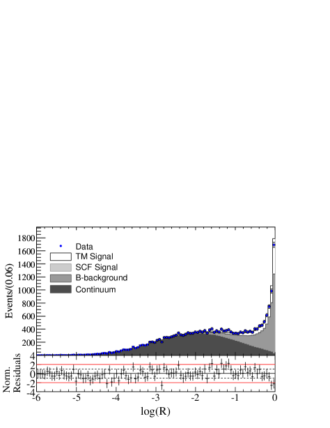
Figure 2: Distributions of the logarithm of likelihood ratio ()
for all events entering the fit (left)
and in the signal-like region (right).
In the right hand side plot, a veto in the , ,
and bands has been applied.
Points with error bars give
the on-resonance data. The solid histogram shows the
projection of the fit result. The dark,
medium, and light shaded areas represent respectively the contribution
from continuum events, the sum of continuum events
and the background expectation, and the sum of these and
the misreconstructed signal events. The last contribution is hardly visible due to its
small fraction. Below each bin are shown the residuals, normalized in error units.
The parallel dotted and full lines are the and deviations.
Points, histograms, shaded areas, and residual plots have similar definitions
in Fig. 3 to 8
Table 4:
Results of fit to data for the isobar amplitudes with statistical uncertainties. Both solutions are shown.
Solution I
Solution II
Isobar Amplitude
Magnitude
Phase (∘)
Magnitude
Phase (∘)
The standard and square Dalitz plots of the selected data sample are shown in Fig. 1.
The maximum-likelihood fit of candidates results in a event yield of
and a continuum yield of , where the uncertainties are statistical only.
The remaining number of events is covered by the yields of backgrounds from charged and neutral decays,
where the dominant contributions are and events.
When the fit is repeated starting from input parameter values randomly chosen within
wide ranges above and below the nominal values for the magnitudes and within the
interval for the phases, we observe convergence toward two solutions with
minimum values of the negative log likelihood function
that are equal within units.
In the following, we refer to them as solution I (the global minimum) and solution II (a local minimum).
Between the two solutions, the fit values for most free parameters are very similar. Exceptions occur among isobar
parameters, and most particularly isobar phases, some of which can differ significantly.
For a given event , we define the likelihood ratio as
(see Eq. (26) and explanations below).
Figure 2 shows distributions of for all
the events entering the fit, and for the signal-like region.
We obtain signal enriched samples that are used in some of the figures below,
by removing events with small values of
; in each case is computed excluding the variable being plotted.
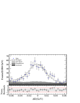
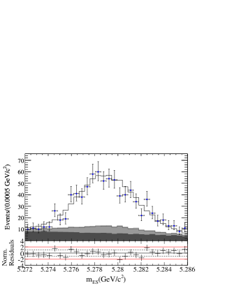
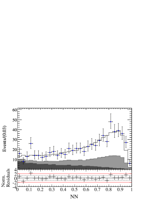
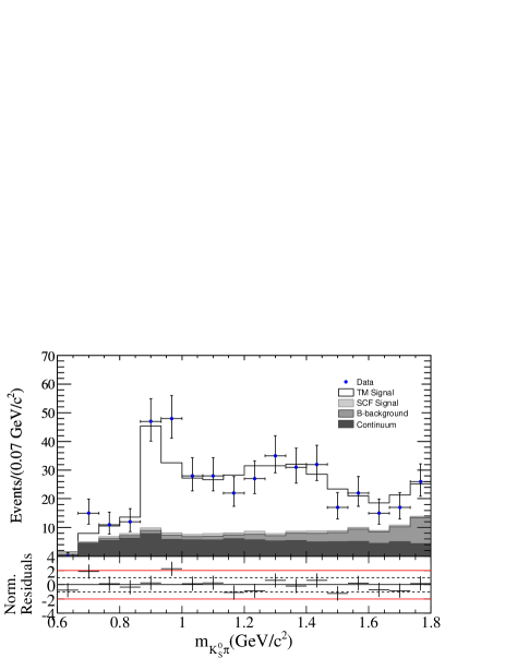
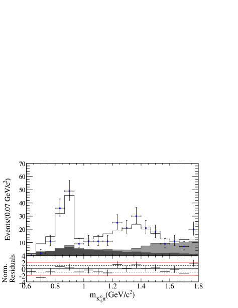
Figure 3 shows
distributions of , , and the NN output which are enhanced in signal content by requirements on
.
Figures 4 to 7
show similar distributions for , , and .
These distributions illustrate the good quality of the fit in the signal-enhanced regions.
Signal enriched distributions of and asymmetry for events in the regions of and
are shown in Fig. 8.
In the fit, we measure directly the relative magnitudes and phases
of the different components of the signal model. The magnitude and phase of the amplitude are fixed to and , respectively, as a reference.
The results corresponding to the two solutions
are given together with their statistical uncertainties in Table 4.
The full (statistical, systematic and model dependent) correlation matrices between the magnitudes and the phases for the two solutions are given in the Appendix.
The measured relative amplitudes , where the index represents an intermediate
resonance, are used to extract the Q2B parameters defined below.
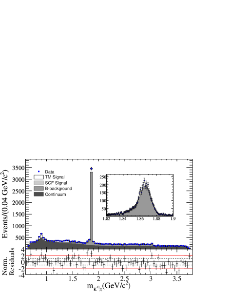
Figure 3: Distributions of (left),
(center), and output (right) for a sample
enhanced in signal with a requirement on the likelihood ratio
computed without the variable being plotted. In each case the applied cut rejects of continuum background,
while retaining of signal for and , and for . A veto in the and bands has been applied.
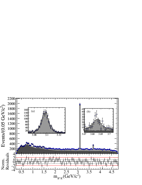
Figure 4:
Spectra of (left) and symmetrized (right)
for the whole data sample.
For , the insets show the region (a)
and in the region (b).
The symmetrized is obtained by folding
the SDP with respect to the variable at .
The inset shows the region.
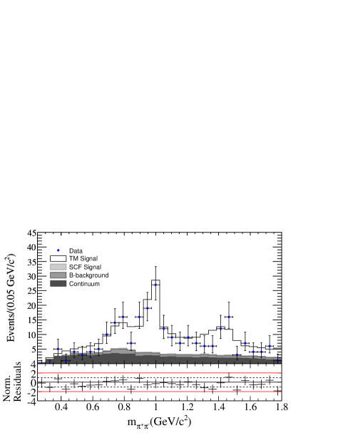
Figure 5: Distribution of for a sample
enhanced in signal, showing the and
signal region for positive (left) and negative (right) helicity.
The contribution from and are also visible.
A veto in the band has been applied.
The and DP PDFs have been
excluded from the likelihood ratio used to enhance the sample in signal events.
The cut on retains of signal, while rejecting of continuum.
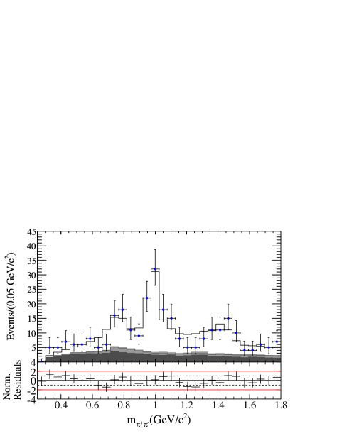
Figure 6:
Distributions of for a sample
enhanced in signal, showing the
and signal region for positive (left) and negative (right)
helicity.
A veto in the and bands has been applied.
The and DP PDFs have been excluded
from the definition of the likelihood ratio used to enhance
the sample in signal events.
The cut on retains of signal while rejecting of continuum.
An interference between the vector and scalar is apparent through a positive
(negative) forward-backward asymmetry
below (above) the .
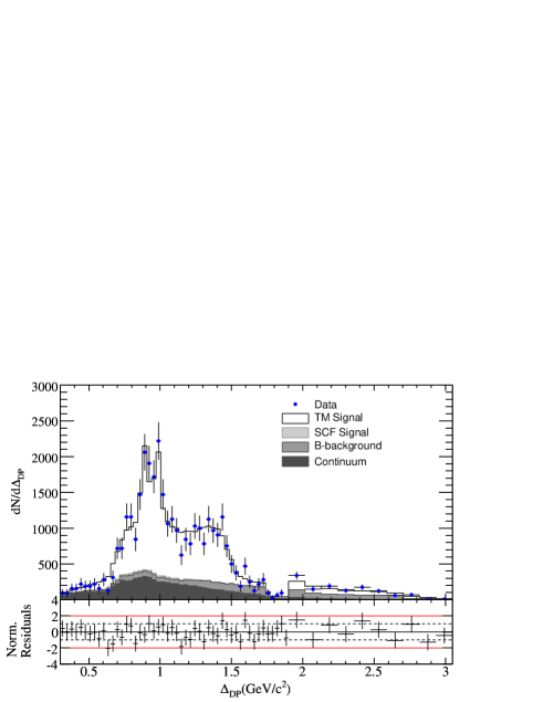
Figure 7:
Distributions of the variable, for a sample enhanced in signal.
The variable is defined as
.
Small (large) values of correspond to the edges (center) of the DP.
On the left (right) side of the figure, for (),
the dominant contribution to the signal is from the light resonances (the NR) component of the signal model.
A veto in the , , and bands has been applied.
The and DP PDFs have been
excluded from the likelihood ratio used to enhance the sample in signal events.
The cut on retains of signal while rejecting of continuum.
Figure 8: Distributions of when the is a (top), (middle), and the derived asymmetry (bottom).
Plots on the left (right) hand side, correspond to events in the () region.
These distributions correspond to samples where the and
bands are removed from the DP, and the and DP PDFs have been
excluded from the likelihood ratio used to enhance the sample in signal events.
The cut on retains of signal while rejecting of continuum.
For a resonant decay mode
which is a eigenstate,
the following Q2B parameters are extracted:
the angle
defined as
(34)
and the direct and mixing-induced asymmetries, defined as:
(35)
(36)
For a flavor-specific resonant decay mode such as , it is customary to define
the direct asymmetry parameter as:
(37)
For a pair of resonances and ,
the phase
relating their amplitudes and , defined as
(38)
can be accessed by exploiting the interference pattern in the DP areas where and overlap;
correspondingly, the phase
for the -conjugated amplitudes and is
(39)
From these two phases, the difference , can be extracted. This parameter
is a direct violation observable, and can only be accessed
in an amplitude analysis.
For a resonant decay mode , the phase relating its amplitude to
its charge conjugate is defined as
(40)
here it is worth recalling that we use a
convention in which the decay amplitudes have absorbed the phase from mixing,
and so the phase of is implicit in the parameter.
Although the definition of this parameter is technically similar to the
phase defined in Eq. (34), they differ in their physical
interpretation. The parameter quantifies the time-dependent mixing-induced asymmetry, and therefore is most relevant for the eigenstate modes, such as and .
On the other hand the parameter concerns mostly flavor-specific
modes, such as , for which there is no interference between decays with and without
mixing. For such modes, sensitivity to is provided indirectly by the interference
pattern of the resonance with other
modes that are accessible both to and decays.
We also extract the relative fit fraction of a Q2B channel , which is calculated as:
(41)
where the terms
(42)
are obtained by integration over the complete Dalitz plot.
The total fit fraction is defined as the algebraic sum of all fit fractions. This quantity is not
necessarily unity due to the potential presence of net constructive or destructive interference.
Using the relative fit fractions, we calculate the branching fraction for the intermediate mode as
(43)
where is the total inclusive branching fraction
(44)
We compute the average efficiency, , by weighting MC events with the measured
intensity distribution of signal events, . The term is the total number of pairs in the sample.
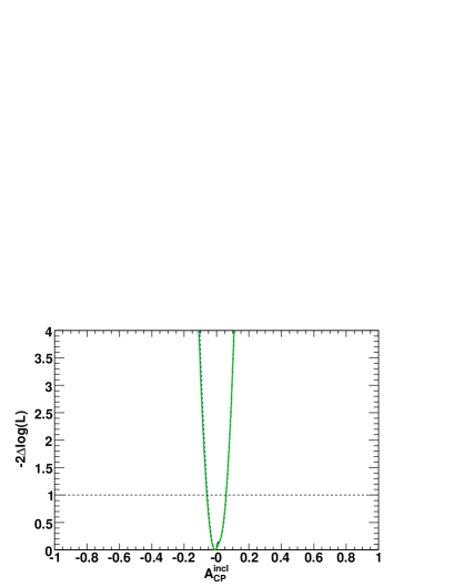
Finally, we use the following integrals of amplitudes over the complete Dalitz plot to measure the inclusive direct -asymmetry:
(45)
The Q2B parameters and fit fractions are given in Table 5,
together with their statistical and systematic errors.
The branching fractions are shown in Table 6.
Table 5:
Summary of measurements of the Q2B parameters for solutions I and II.
The first uncertainty is statistical, the second is systematic, and the third represents the DP signal model dependence.
We also show the total (statistical and systematic) linear correlations between the parameters () and .
Phases are given in degrees and s in percent.
Parameter
Solution I
Solution II
total
Table 6:
Summary of measurements of branching fractions averaged over charge conjugate states. The quoted numbers were obtained by multiplying the corresponding fit fractions by the measured inclusive branching fraction. denotes an intermediate resonant state and stands for a final state hadron: a charged pion or a . To correct for the secondary branching fractions we used the values from Ref. Amsler et al. (2008) and . The first uncertainty is statistical, the second is systematic, and the third represents the DP signal model dependence. The fourth errors, when applicable, are due to the uncertainties on the
secondary branching fractions. The quoted central values correspond to the global minimum, and errors account for the presence of the second solution.
Mode
Inclusive
flat NR
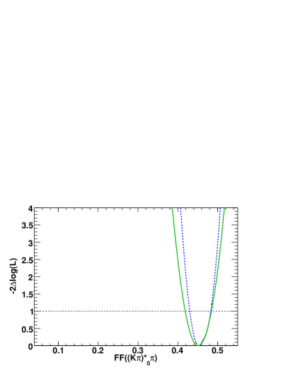
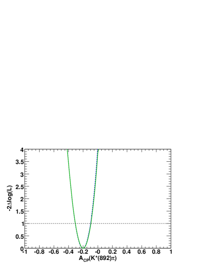
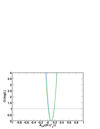
To extract the statistical uncertainties on the Q2B parameters we perform
likelihood scans, not relying on any assumption about the shape of the
likelihood function.
Since the Q2B parameters are not directly used in the fit, we instead must
perform the scan fixing one or two parameters among the signal model
magnitudes and phases. These are chosen in such a way that the resulting
likelihood curve can be trivially interpreted in terms of the Q2B parameter
of interest. In each case the chosen parameters are fixed at several consecutive
values, for each of which the fit to the data is repeated.
The error on the Q2B parameter is determined by the points, or the contour,
where the function changes by one unit with respect to its
minimum value.
Systematic uncertainties are discussed in Sec. VII.
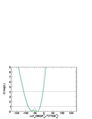
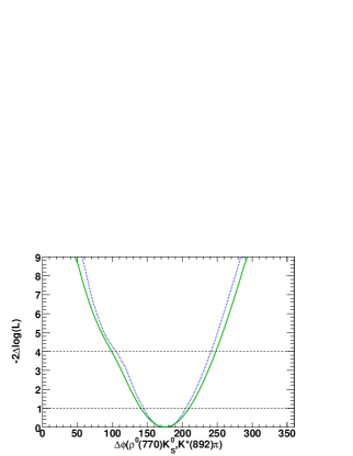
Results of the likelihood scans in terms of are shown in
Fig. 9 to 16.
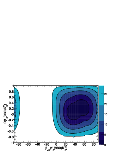
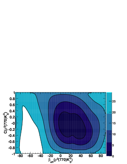
The measurements of time-dependent -violation in the
and modes are presented as two-dimensional likelihood scans in the
plane, shown in Fig. 9.
The scans are displayed as confidence level contours after two-dimensional
convolution with the covariance matrix of systematic uncertainties.
On the same figure are also displayed the one-dimensional likelihood scans of .
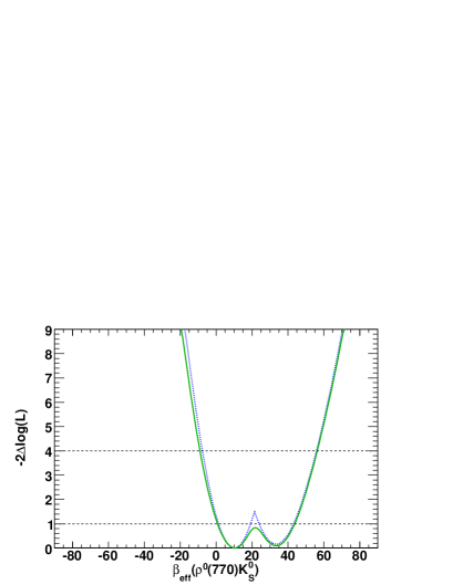
For the two solutions lie below and above degrees and correspond very closely
to the trigonometric ambiguity between a given value of and
(mirror solutions). On the other hand, for both solutions are below degrees.
In this case the local solutions corresponding to the trigonometric ambiguities of the two observed
solutions are suppressed at and standard deviations, respectively.
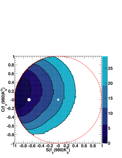
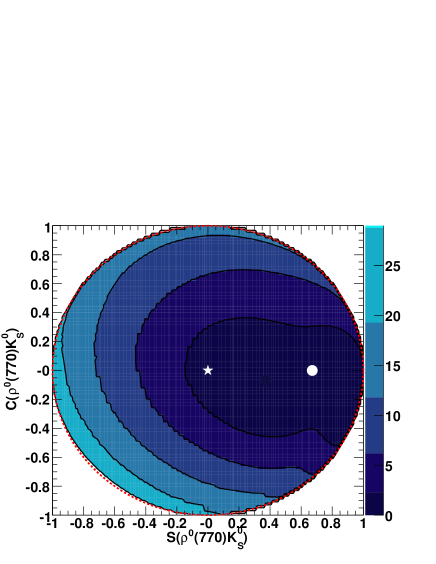
The plane can be transformed to the more familiar
plane using Eq. (34) to (36). The corresponding two-dimensional contours are shown
in Fig. 10. While a part of the information on the phases is lost,
this representation has nonetheless the advantage
of allowing direct comparison with the measurement of and in
modes. For , the results agree with the expectation based on
to ; for the agreement is better than
.
For the measured values of for ,
conservation is excluded
at .
For , the measurement of
is consistent with conservation within .
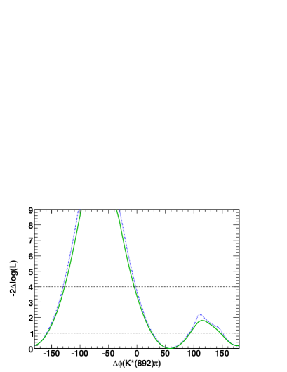
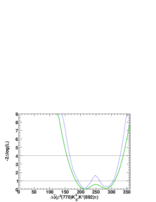
The measurement of the phase is
presented as a one-dimensional likelihood scan in Fig. 11.
For this flavor-specific mode, there is virtually no
region in phase space that is accessible both to and ;
thus, sensitivity to this phase difference is limited.
Simulation shows that
interference of the with the and modes
(for which and amplitudes interfere via mixing) provides most of the
sensitivity to ; unfortunately, the overlap in phase
space of these resonances is small.
As a consequence,
only the interval is excluded at confidence level.
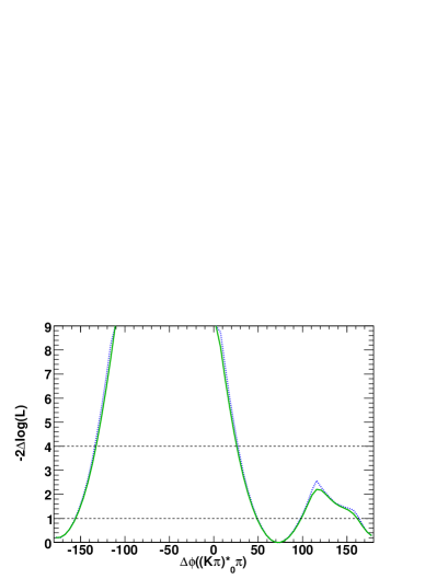
Figure 11 also shows the measurement of the similar
phase difference for the component. As for , the measurement
sets no strong constraint on this phase. Only the interval is excluded at
confidence level.
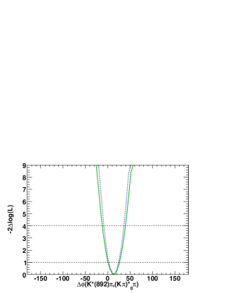
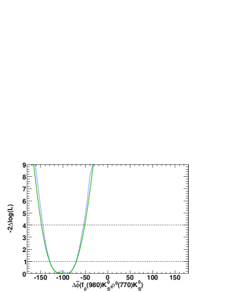
In contrast, due to the sizable overlap in phase space between the S- and P- waves of the same charge,
the relative phases
are measured to including systematics.
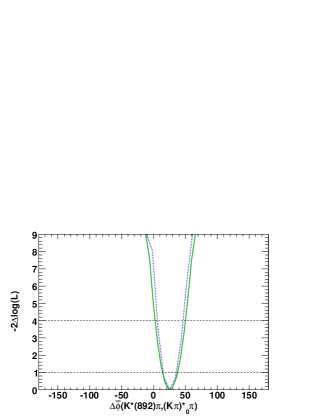
The one-dimensional scans are shown in Fig. 12. The
associated
observable is compatible with conservation.
Figure 12 also shows the scans for ,
, and their corresponding -conjugates.
It is clear from this figure and from Table V that the phases for the former are measured to a better accuracy. This is due to the larger overlap in phase space between the and the . In both cases
the associated
observables are compatible with conservation.
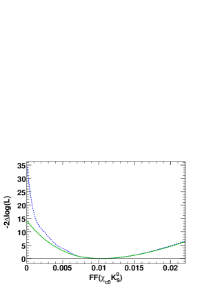
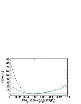
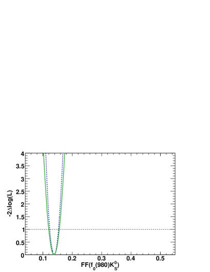
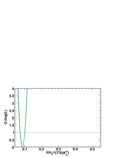
For the remaining resonant modes in the signal DP model:
, , NR, and , we scan the
likelihood as a function of the corresponding fit fractions. These scans are shown in
Fig. 13. We obtain
a total (statistical and systematic) significance of and
standard deviations for the NR and components, respectively.
The significance for the sum of fit fractions of the and components is standard deviations
while their individual significances are and , respectively.
The component is modeled in our analysis by the LASS parametrization Aston et al. (1988),
which consists of a NR effective range term plus a relativistic Breit-Wigner term for
the resonance. We separate from the corresponding branching fraction, quoted in
Table 6, the contribution of the resonance and find it to be
.
This value is corrected for the secondary branching
fraction using from Ref. Amsler et al. (2008) and the isospin relation
.
The first uncertainty is statistical, the second is systematic, the third represents the DP signal model
dependence, and the fourth is due to the uncertainty on the secondary branching fraction.
In addition we calculate the total NR contribution by combining coherently the effective range
part of the LASS parametrization and the flat phase-space NR component.
We find this total NR fit fraction to be
.
Note that this number accounts for the destructive interference between the two NR terms.
The corresponding branching fraction is
.
As a validation of our treatment of the time-dependence, we allow
and to vary in the fit. We find
and
while the remaining free parameters are consistent with the nominal fit. The numbers
for and are in agreement with current world averages Barberio et al. (2008).
In addition we perform a fit floating the parameters for
and events. We
find and for
and respectively. These numbers are
in agreement with the current world average Barberio et al. (2008).
Signal enhanced distributions of and the asymmetry for events in the
region are shown in Fig. 17.
To validate the SCF modeling, we leave the average SCF fractions per tagging
category free to vary in the fit and find results that are consistent
with the MC estimation.
As a further cross-check of the results,
we performed an independent analysis and obtained compatible results del Amo Sanchez (2007).
The main differences between this cross-check analysis and the one presented
here were the use of a Fisher discriminant instead of a NN, the removal of
bands in invariant mass to cut away the , and contributions, and the use of Cartesian
isobar parameters.
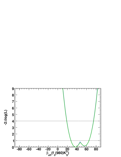
Figure 9:
Two-dimensional scans of as a function of
and (top) and the one-dimensional scans as a function of (bottom)
for the (left) and (right) isobar components.
The value is computed including systematic uncertainties.
On the two-dimensional scans, shaded areas, from the darkest to the lightest, represent
the one to five standard deviations contours.
The statistical (dashed line), and total (solid line) are shown on the one-dimensional scans,
where horizontal dotted lines mark the one and two standard deviation levels.
Figure 10:
Two-dimensional scans of as a function of
, for the (left) and (right) isobar components.
The value is computed including systematic uncertainties.
Shaded areas, from the darkest to the lightest, represent the one to five standard deviations contours.
The () marks the expectation based on
the current world average from
modes Barberio et al. (2008) (zero point). The dashed circle represents the physical border .
Figure 11: Statistical (dashed line) and total (solid line) scans of
as a function of the relative phases
(left) and (right). Horizontal dotted lines mark the
one and two standard deviation levels.
Figure 12:
Statistical (dashed line) and total (solid line) scans of
as a function of the phase differences
(left),
(middle), and
(right).
The top (bottom) row shows () candidates.
Horizontal dotted lines mark the
one and two standard deviation levels.
Figure 13:
Statistical (dashed line) and total (solid line) scans in terms of
as a function of the fit fractions of the
component (left), the sum of fit fractions of the
and components (center), and the flat phase space NR component (right).
These scans are used to extract the probability of null values of these fit fractions.
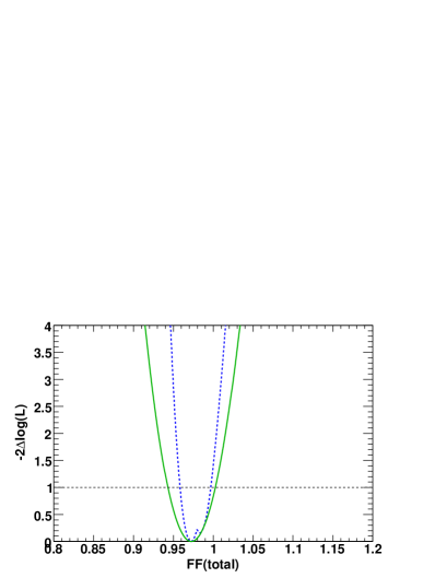
Figure 14:
Statistical (dashed line) and total (solid line) scans of
as a function of the total fit fraction (left) and the inclusive direct -asymmetry (right).
A horizontal dotted line marks the one standard deviation level.
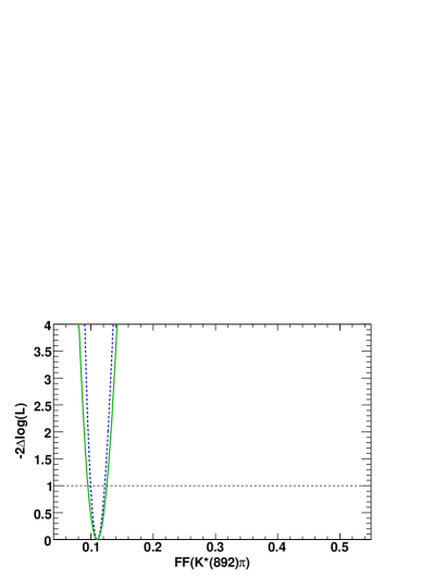
Figure 15:
Statistical (dashed line) and total (solid line) scans of
as a function of the fit fractions
(top left), (top right), (bottom left),
and (bottom right).
A horizontal dotted line marks the one standard deviation level.
Figure 16:
Statistical (dashed line) and total (solid line) scans of
as a function of the direct asymmetries
(left) and
(right).
A horizontal dotted line marks the one standard deviation level.
Figure 17: Distributions of when the is a (top), (middle), and the derived asymmetry (bottom)
for events in the region. The solid line is the total PDF
and the points with error bars represent data.
VII SYSTEMATIC STUDIES
Table 7:
Summary of systematic uncertainties on Q2B parameters. Errors on relative fractions ( and phases) are given in percent (degrees).
Parameter
DP Model
Lineshape
Fit Bias
Background
Other
Total
0.04
0.02
0.01
0.01
0.02
0.05
0.6
0.69
0.5
0.07
0.01
1.03
2.1
1.9
0.1
0.2
0.3
2.9
0.03
0.04
0.01
0.06
0.06
0.10
0.23
0.31
0.3
0.09
0.15
0.52
1.8
2.2
0.1
1.2
1.7
3.5
0.02
0.01
0.01
0.01
0.01
0.02
0.8
0.13
0.4
0.03
0.43
1.00
8.1
2.8
0.1
1.4
3.3
9.3
0.02
0.01
0.01
0.01
0.02
0.03
0.90
0.39
1.8
0.12
0.33
2.08
4.4
2.4
0.1
1.3
3.0
6.0
0.07
0.04
0.01
0.05
0.06
0.11
0.69
0.16
0.09
0.02
0.19
0.74
0.09
0.03
0.01
0.01
0.03
0.10
0.87
0.28
0.14
0.02
0.17
0.94
0.04
0.01
0.01
0.01
0.07
0.08
0.60
0.86
0.5
0.12
1.62
2.00
0.05
0.02
0.01
0.01
0.02
0.06
0.09
0.06
0.04
0.01
0.01
0.11
0.01
0.01
0.01
0.01
0.01
0.01
1.15
0.55
2.0
0.08
0.36
2.40
4.4
2.6
0.1
3.4
4.3
7.5
12.7
3.0
0.1
3.6
7.3
15.4
8.7
8.5
0.1
3.9
3.7
13.3
4.7
0.7
0.1
0.3
4.6
6.6
Signal Yield
31.7
5.8
14.0
3.3
23.0
42.1
To estimate the contribution to decay via other
resonances, we first
fit the data including these other decays in the fit model.
We consider possible resonances,
including , , ,
, , , ,
,
and a low mass . A relativistic Breit–Wigner lineshape is used to parameterize these additional
resonances, with masses and widths from Ref. Amsler et al. (2008).
As a second step we simulate high statistic samples of events, using a model based
on the previous fits, including the additional resonances. Finally, we
fit these simulated samples using the nominal signal model.
The systematic effect (contained in the “DP Model” field in
Table 7) is taken from the difference observed between the generated and fitted values.
We quote this DP model
uncertainty separately from other systematics.
We vary the mass, width,
and any other parameters of all isobar fit components within their errors,
as quoted in Table 1, and assign the observed
differences in the measured amplitudes as systematic uncertainties
(“Lineshape” in Table 7).
To validate the fitting tool, we perform fits on large MC samples
of fully-reconstructed events with
the measured proportions of signal, continuum, and background events.
No significant biases are observed in these fits and therefore no corrections are applied.
The statistical uncertainties on the fit parameters are taken as systematic uncertainties
(“Fit Bias” in Table 7).
Another major source of systematic uncertainty is the background model.
The expected event yields from the background modes are varied according
to the uncertainties in the measured or estimated branching fractions.
Since background modes may exhibit violation, the corresponding
parameters are varied within their uncertainties, or, if unknown, within the physical range.
As is done for the signal PDFs, we vary the resolution parameters and
the flavor-tagging parameters within their uncertainties and assign
the differences observed in these fits with respect to the nominal fit
as systematic errors.
These errors are
listed as “ Background ” in Table 7.
Other systematic effects are much less important for the measurements
of the amplitudes and are combined in
the “Other” field in Table 7. Details are given
below.
The parameters of the continuum PDFs are determined by the fit. No additional systematic
uncertainties are assigned to them. An exception to this is the DP
PDF: to estimate the systematic
uncertainty from the sideband extrapolation, we use large
samples of MC data ().
We compare the distributions of and between sidebands at
different ranges in and find the two such sidebands that show the
maximum discrepancy. We assign as systematic uncertainty the effect seen
when weighting the continuum DP PDF by the ratio of these two data sets.
The uncertainties associated with and are
estimated by varying these parameters within the uncertainties
on the world average Amsler et al. (2008).
The signal PDFs for the resolution and tagging fractions
are determined from fits to a control sample
of fully reconstructed decays to exclusive final states with
charm, and the uncertainties are obtained by varying the parameters
within the statistical uncertainties.
Finally, the uncertainties due to particle
identification, tracking efficiency corrections, reconstruction, and the calculation
of are , , , and , respectively.
These contribute only to the branching fraction systematic uncertainties.
The average fraction of misreconstructed signal events () predicted by the MC
simulation has been verified with fully reconstructed
events Aubert et al. (2007b). No significant differences between data and
the simulation were found.
To estimate
a systematic uncertainty from
, we vary these fractions, for all tagging categories.
Tagging efficiencies, dilutions, and biases for signal events
are varied within their experimental uncertainties.
VIII SUMMARY
We have presented results from a time-dependent Dalitz plot analysis of decays
obtained from a data sample of million decays.
Using an amplitude analysis technique,
we measure pairs of relative magnitudes and phases for the different resonances,
taking advantage of the interference between them in the Dalitz plot.
From the measured decay amplitudes, we derive the Q2B parameters of the resonant decay modes.
Two solutions, with equivalent goodness-of-fit, were found.
Including systematic and Dalitz plot model uncertainties, the combined confidence interval
for the measured values of
in decays to is
at C.L.
conservation in decays to is excluded at
, including systematics. For decays to
, the combined confidence interval is
at C.L.
These results are both consistent with the measurements in modes.
In decays to , we find
.
For the relative phase between decay amplitudes of and ,
we exclude the interval at C.L.
This last result, combined with measurements of branching ratios, direct asymmetries, and relative
phases in and , plus a theoretical hypothesis on the
contributions of electroweak penguins to the decay amplitudes, can be used to set non-trivial constraints
on the CKM parameters by following the methods proposed
in Refs. Deshpande et al. (2003); Ciuchini et al. (2006); Gronau et al. (2007); Lipkin et al. (1991).
ACKNOWLEDGMENTS
We are grateful for the
extraordinary contributions of our PEP-II colleagues in
achieving the excellent luminosity and machine conditions
that have made this work possible.
The success of this project also relies critically on the
expertise and dedication of the computing organizations that
support BABAR.
The collaborating institutions wish to thank
SLAC for its support and the kind hospitality extended to them.
This work is supported by the
US Department of Energy
and National Science Foundation, the
Natural Sciences and Engineering Research Council (Canada),
the Commissariat à l’Energie Atomique and
Institut National de Physique Nucléaire et de Physique des Particules
(France), the
Bundesministerium für Bildung und Forschung and
Deutsche Forschungsgemeinschaft
(Germany), the
Istituto Nazionale di Fisica Nucleare (Italy),
the Foundation for Fundamental Research on Matter (The Netherlands),
the Research Council of Norway, the
Ministry of Education and Science of the Russian Federation,
Ministerio de Educación y Ciencia (Spain), and the
Science and Technology Facilities Council (United Kingdom).
Individuals have received support from
the Marie-Curie IEF program (European Union) and
the A. P. Sloan Foundation.
APPENDIX
The full (statistical, systematic, and model dependence) correlation matrices of the isobar parameters for
solutions I and II are given in Tables 8 and 9, respectively.
The tables are organized in blocks for , , , and .
Here, the abbreviations , , , , , , , and represent the components , , , , , , nonresonant, and , respectively.
Table 8:
Full correlation matrix for the isobar parameters of solution I. The entries are given in percent. Since the matrix is symmetric, all elements above the diagonal are omitted.
Table 9:
Full correlation matrix for the isobar parameters of solution II. The entries are given in percent. Since the matrix is symmetric, all elements above the diagonal are omitted.
References
Cabibbo (1963)
N. Cabibbo,
Phys. Rev. Lett. 10,
531 (1963).
Kobayashi and Maskawa (1973)
M. Kobayashi and
T. Maskawa,
Prog. Theor. Phys. 49,
652 (1973).
Barberio et al. (2008)
E. Barberio et al.
(Heavy Flavor Averaging Group - HFAG)
(2008), eprint arXiv:0808.1297 [hep-ex].
Grossman et al. (2003)
Y. Grossman,
Z. Ligeti,
Y. Nir, and
H. Quinn,
Phys. Rev. D68,
015004 (2003).
Gronau et al. (2004a)
M. Gronau,
Y. Grossman, and
J. L. Rosner,
Phys. Lett. B579,
331 (2004a).
Gronau et al. (2004b)
M. Gronau,
J. L. Rosner,
and J. Zupan,
Phys. Lett. B596,
107 (2004b).
Cheng et al. (2005a)
H.-Y. Cheng,
C.-K. Chua, and
A. Soni,
Phys. Rev. D72,
014006 (2005a).
Gronau and Rosner (2005)
M. Gronau and
J. L. Rosner,
Phys. Rev. D71,
074019 (2005).
Beneke (2005)
M. Beneke,
Phys. Lett. B620,
143 (2005).
Engelhard et al. (2005)
G. Engelhard,
Y. Nir, and
G. Raz,
Phys. Rev. D72,
075013 (2005).
Cheng et al. (2005b)
H.-Y. Cheng,
C.-K. Chua, and
A. Soni,
Phys. Rev. D72,
094003 (2005b).
Williamson and Zupan (2006)
A. R. Williamson
and J. Zupan,
Phys. Rev. D74,
014003 (2006).
Gershon and Hazumi (2004)
T. Gershon and
M. Hazumi,
Phys. Lett. B596,
163 (2004).
Garmash et al. (2004)
A. Garmash et al.
(Belle), Phys. Rev.
D69, 012001
(2004).
Aubert et al. (2007a)
B. Aubert et al.
(BABAR), Phys. Rev. Lett.
99, 161802
(2007a).
Wolfenstein (1983)
L. Wolfenstein,
Phys. Rev. Lett. 51,
1945 (1983).
Buras et al. (1994)
A. J. Buras,
M. E. Lautenbacher,
and
G. Ostermaier,
Phys. Rev. D50,
3433 (1994).
Deshpande et al. (2003)
N. G. Deshpande,
N. Sinha, and
R. Sinha,
Phys. Rev. Lett. 90,
061802 (2003).
Ciuchini et al. (2006)
M. Ciuchini,
M. Pierini, and
L. Silvestrini,
Phys. Rev. D74,
051301 (2006).
Gronau et al. (2007)
M. Gronau,
D. Pirjol,
A. Soni, and
J. Zupan,
Phys. Rev. D75,
014002 (2007).
Lipkin et al. (1991)
H. J. Lipkin,
Y. Nir,
H. R. Quinn, and
A. Snyder,
Phys. Rev. D44,
1454 (1991).
Dalseno et al. (2009)
J. Dalseno et al.
(Belle), Phys. Rev.
D79, 072004
(2009).
Aubert et al. (2006)
B. Aubert et al.
(BABAR), Phys. Rev.
D73, 031101
(2006).
Garmash et al. (2007)
A. Garmash et al.
(Belle), Phys. Rev.
D75, 012006
(2007).
Chang et al. (2004)
P. Chang et al.
(Belle), Phys. Lett.
B599, 148 (2004).
Aubert et al. (2008a)
B. Aubert et al.
(BABAR), Phys. Rev.
D78, 052005
(2008a).
Aubert et al. (2008b)
B. Aubert et al.
(BABAR), Phys. Rev.
D78, 012004
(2008b).
Garmash et al. (2006)
A. Garmash et al.
(Belle), Phys. Rev. Lett.
96, 251803
(2006).
Chang et al. (2008)
Q. Chang,
X.-Q. Li, and
Y.-D. Yang,
JHEP 0809, 038
(2008).
Blatt and Weisskopf (1952)
J. Blatt and
V. E. Weisskopf,
Theoretical Nuclear Physics (J.
Wiley (New York), 1952).
Amsler et al. (2008)
C. Amsler et al.
(Particle Data Group), Phys.
Lett. B667, 1
(2008).
Flatte (1976)
S. M. Flatte,
Phys. Lett. B63,
224 (1976).
Gounaris and Sakurai (1968)
G. J. Gounaris and
J. J. Sakurai,
Phys. Rev. Lett. 21,
244 (1968).
Aston et al. (1988)
D. Aston et al.
(LASS), Nucl. Phys.
B296, 493 (1988).
Bugg (2003)
D. V. Bugg,
Phys. Lett. B572,
1 (2003).
Ablikim et al. (2005)
M. Ablikim et al.
(BES), Phys. Lett.
B607, 243 (2005).
Aubert et al. (2005a)
B. Aubert et al.
(BABAR), Phys. Rev.
D72, 052002
(2005a).
Aubert et al. (2002)
B. Aubert et al.
(BABAR), Nucl. Instrum. Meth.
A479, 1 (2002).
Gay et al. (1995)
P. Gay,
B. Michel,
J. Proriol, and
O. Deschamps
(1995), prepared for 4th International
Workshop on Software Engineering and Artificial Intelligence for High-energy
and Nuclear Physics (AIHENP 95), Pisa, Italy, 3-8 April 1995.
Aubert et al. (2005b)
B. Aubert et al.
(BABAR), Phys. Rev. Lett.
94, 161803
(2005b).
Gardner and Tandean (2004)
S. Gardner and
J. Tandean,
Phys. Rev. D69,
034011 (2004).
Aubert et al. (2007b)
B. Aubert et al.
(BABAR), Phys. Rev.
D76, 012004
(2007b).
Oreglia (1980)
M. Oreglia, Ph.D. thesis,
SLAC-R-0236 (1980),
Appendix D.
Gaiser (1982)
J. Gaiser, Ph.D. thesis,
SLAC-R-0255 (1982),
Appendix F.
Skwarnicki (1986)
T. Skwarnicki, Ph.D. thesis,
DESY-F31-86-02 (1986),
Appendix E.
Albrecht et al. (1990)
H. Albrecht et al.
(ARGUS), Z. Phys.
C48, 543 (1990).
del Amo Sanchez (2007)
P. del Amo Sanchez, Ph.D.
thesis, BABAR-THESIS-07-007 (2007).