The Tidal Tails of Globular Cluster Palomar 5 Based on Neural Networks Method

Abstract

The Sixth Data Release (DR6) in the Sloan Digital Sky Survey (SDSS) provides more photometric regions, new features and more accurate data around globular cluster Palomar 5. A new method, Back Propagation Neural Network (BPNN), is used to estimate the probability of cluster member to detect its tidal tails. Cluster and field stars, used for training the networks, are extracted over a $40\times 20$ deg² field by color-magnitude diagrams (CMDs). The best BPNNs with two hidden layers and Levenberg-Marquardt (LM) training algorithm are determined by the chosen cluster and field samples. The membership probabilities of stars in the whole field are obtained with the BPNNs, and contour maps of the probability distribution show that a tail extends $5.42\dg$ to the north of the cluster and a tail extends $3.77\dg$ to the south. The whole tails are similar to those detected by Odenkirchen et al. (2003), but no longer debris of the cluster is found to the northeast of the sky. The radial density profiles are investigated both along the tails and near the cluster center. Quite a few substructures are discovered in the tails. The number density profile of the cluster is fitted with the King model and the tidal radius is determined as $14.28^{\prime}$. However, the King model cannot fit the observed profile at the outer regions ($R>8^{\prime}$) because of the tidal tails generated by the tidal force. Luminosity functions of the cluster and the tidal tails are calculated, which confirm that the tails originate from Palomar 5.

1 Introduction

Globular clusters (GCs) are the oldest populations in the Galaxy. Most of GCs, which formed in the early days of the Galaxy, have been destroyed by various mechanisms (Wu et al., 2003). Mass loss from stellar evolution is very important during the first $\sim 1$ Gyr of cluster evolution, and most of low mass clusters have been dissolved during this early phase. For survival clusters, their evolutions will be dominated by the internal dynamical processes caused by encounters between cluster stars (the two-body relaxation) (Spitzer, 1987). GCs in the Galaxy have elliptical orbits, and some of them can move into the central region of the Galaxy with perigalactic distances less than $\sim 1$ kpc (Wu et al., 2004). When a cluster crosses the bulge or disk of the Galaxy with timescale shorter than its internal dynamical time, the cluster stars will gain energy and speed up the evaporation. Such an interaction is referred to as the tidal shock (Spitzer, 1987). Stars evaporating from the cluster due to two-body relaxation or tidal shocks, will not leave the cluster and merge into the Galactic field immediately. They will move along the same orbit of the cluster and form the ‘tidal tail’ of the cluster.

Grillmair et al. (1995) examined the outer structures of 12 Galactic globular clusters using star-count analysis with deep, two-color photographic photometry. They found that most of their sample clusters show extra-tidal wings in their surface density profiles. Two-dimensional surface density maps for several clusters indicate the expected appearances of tidal tails. Leon et al. (2000) used large-field photographic photometry of 20 globular clusters to investigate the presence of tidal tails around these clusters; in this study, star-count analysis and wavelet transform were used to detect the weak structures formed by the stars that previously are members of the clusters; and most of globular clusters in their sample display large and extended tidal tails, which exhibit projected directions towards the Galactic center.

The studies of Grillmair et al. (1995) and Leon et al. (2000) are all based on photographic observations covering large areas around the clusters. The low signal-to-noise in the photographic photometry and serious contaminants from the background galaxies make the detected tidal tails in some clusters uncertain. The SDSS can provide large, deep CCD imaging in five passbands coving 10,000 deg² in the sky. The SDSS can also separate the stars and galaxies very well and is very efficient in detecting tidal tails around globular clusters in the Galaxy. Using SDSS data, well-defined tidal tails in some globular clusters have been identified: Palomar 5 (Odenkirchen et al., 2001, 2003; Grillmair & Dionatos, 2006), NGC5466 (Belokurov et al., 2006; Grillmair & Johnson, 2006), and NGC 5053 (Lauchner et al., 2006).

In above mentioned studies, Palomar 5 is a prominent object. It is a remote globular cluster located at a distance of 23.2 kpc from the Sun and has a tidal radius of about 16.3 arcmin (Harris, 1996). Using the ESO and SERC survey plates covering about $2.0\dg\times 2.0\dg$ in $R$ and $J$ filters, Leon et al. (2000) searched the tidal tails around this cluster and found that the detected structures outside this cluster are strongly biased by the background galaxy clusters appearing in the field, and it is difficult to derive any conclusions on the genuine location of stars in the tidal tails of this cluster.

Using SDSS data concentrating on Palomar 5 in a region with right ascensions $226\dg\leq\alpha\leq 232\dg$ and declinations $-1.25\dg\leq\delta\leq+1.25\dg$, Odenkirchen et al. (2001) searched the tidal tails of this cluster based on the empirical photometric filtering method of Grillmair et al. (1995). They found two well-defined tidal tails emerging from this cluster to stretch out symmetrically to both sides of the cluster and extend an angle of $2.6\dg$ on the sky. Using the new SDSS data (before the public data release DR1) yielding complete coverage of a region with a $6.5\dg$ to $8\dg$ wide zone along the equator and right ascension from $224\dg$ to $236\dg$, and based on optimal contrast filtering method, Odenkirchen et al. (2003) found that the tidal tails of Palomar 5 have a much larger spatial extent and can be traced about an arc of $10\dg$ on the sky. More recently, using the SDSS DR4 data, Grillmair & Dionatos (2006) applied the optimal contrast filtering method of Odenkirchen et al. (2003) to tracing the tidal tails of Palomar 5 in a region $224\dg<\alpha<247\dg$ and $-3\dg<\delta<+10\dg$, and found the tidal tails to extend to some $22\dg$ on the sky.

Most of the studies are based on star-count analysis in color-magnitude space. While Belokurov et al. (2006) gave us a brand new angle of view to recognize the tidal tails of clusters. Their method is based on an intelligent computing technique, Artificial Neural Networks (ANN), which has been applied in many sorts of areas, such as classification and pattern recognition. In the study of Belokurov et al. (2006), back propagation neural network — the most widely applied ANN — was used to estimate the probability of cluster member for each object in the SDSS 5-band data space. Compared to Odenkirchen et al. (2003), BPNN makes full use of the photometric information, not just one CMD. Therefore, in this paper, we will introduce this method to investigate the tidal tails of Palomar 5, where the DR6 data in a larger region ($40\times 20$ deg²) are used.

In $\S\ref{data}$, we describe the details of the SDSS DR6 and preprocessing of the observed data. Section 3 presents the general idea of BPNN. In $\S\ref{appl}$, we construct BPNNs with the best performances after being trained with properly selected training data, and then we apply them to the tidal tails detection of Palomar 5. Section 5 discusses the profiles and features of the tails. A brief conclusion is given in $\S$6.

2 The Star Sample

2.1 Observations

In this study, the photometric data in the SDSS DR6 are used. The SDSS is a photometric and spectroscopic survey, providing detailed optical images covering more than a quarter of the sky and a 3-dimensional map of about a million galaxies and quasars. A dedicated, 2.5-meter telescope is located on Apache Point, New Mexico, equipped with a 120-megapixel camera and a pair of spectrographs fed by optical fibers measuring more than 600 sources in a single observation. There are 30 photometric CCDs with size $2048\times 2048$ pixels for each. The field of view is $3.0\dg$, and 5 broad band filters with the wavelength ranging from 3000 Å to 10000 Å are used when photometric images are taken. By far, subsequent data releases have been published, including Early Data Release (EDR), DR1, DR2, DR3, DR4, DR5, DR6 and DR7.

DR6 (Adelman-McCarthy et al., 2008) is the first release which has significant changes about the processing software since DR2. For example, calibrations are improved using cross-scans to tie the photometry of the entire survey to each other. The photometric calibration is improved with uncertainties of roughly $1\%$ in $g$, $r$, $i$ and $z$, and $2\%$ in $u$, which are substantially better than the ones in previous data releases. In addition, the magnitude limits are 22.0 for $u$, 22.2 for $g$ and $r$, 21.3 for $i$, and 20.5 for $z$. More importantly, compared with DR4, DR6 includes new observed regions where we can search the tidal tails of Palomar 5.

Odenkirchen et al. (2003) only considered a limited region covering an area of 87 deg² and found the tails extending about an angular distance of $10\dg$. No further investigation in the north, where photometric data exist, was made to see whether the tails are longer. Grillmair & Dionatos (2006) detected a $22\dg$ tidal tails in a larger region. Far from the center of Palomar 5, these newly discovered tails do not appear clearly, since signals and the background noise are so similar. On the other hand, Grillmair & Dionatos (2006) used the DR4, in which a narrow strip ($\alpha>~{}228.5\dg$ and $0.5\dg<\delta<1.5\dg$) stretching to the north tidal tail has no photometric data, while DR6 supplements this area. Therefore, in an area of $40\times 20$ deg² ($220\dg<\alpha<260\dg$ and $-5\dg<\delta<15\dg$), DR6 provides more photometric data. Due to tremendous number of objects included in the area, we partition the whole field into 4 regions equally: R1 (R.A.: $220\dg\sim 230\dg$, Dec.: $-5\dg\sim 15\dg$); R2 (R.A.: $229\dg\sim 240\dg$, Dec.: $-5\dg\sim 15\dg$); R3 (R.A.: $239\dg\sim 250\dg$, Dec.: $-5\dg\sim 15\dg$) and R4 (R.A.: $249\dg\sim 260\dg$, Dec.: $-5\dg\sim 15\dg$), where any two contiguous regions are overlapped by an area of $1\times 20$ deg² in order to avoid bad smoothing at the edges (see $\S\ref{appl}$).

The information, which we need to detect the tidal tails of Palomar 5, includes: coordinate (J2000), point spread function (PSF) magnitude ($r_{\textrm{psf}}$) and exponential model magnitude ($r_{\textrm{exp}}$) of $r$ band, the reddening values and the type of each source. The way to separate stars from galaxies, the definition of $r_{\textrm{psf}}$ and $r_{\textrm{exp}}$, photometric and astrometric data reduction, and relative information can be referred to the works (Lupton et al., 2001; Stoughton et al., 2002; Abazajian et al., 2004). We use so-called Cmodel magnitudes (the default provided values of $ugriz$) as our photometric data, because Cmodel magnitude is the best fit of exponential and de Vaucouleurs models in each band, and it agrees excellently with both PSF magnitude of stars and Petrosian magnitude of galaxies. Even though we only extract stars to check the tidal tails, it’s impossible for us to promise that there are not any miscellaneous galaxies which can not be distinguished by SDSS data reduction piplines. Thus, for uniformity and the validity of the photometry of both stars and galaxies, we choose the universal magnitudes (Cmodel). Reddening corrections for each object are deducted based on the reddening values from Schlegel et al. (1998).

In our selected sky field, we obtain 15,305,060 sources in the catalog, where there are 7,410,896 stars and 7,894,164 galaxies classified by SDSS piplines. There are 5,458,077 sources in R1, 5,508,433 in R2, 4,164,575 in R3 and 173,975 in R4, respectively.

2.2 Data Preprocessing

For source type determination in the SDSS, there are some flaws. For example, occasionally SDSS piplines fail to distinguish blenders and pairs of stars with small separations. Sometimes, the classification scheme regards Seyfert galaxies or QSOs as stars (Stoughton et al., 2002), and overflows of very bright stars are identified as galaxies. Furthermore, due to variations of observing conditions and natural differences in diverse fields, the completeness of object detection is fluctuant. Considering magnitude limits and the situations depicted above, it is necessary to give cutoffs of magnitude to avoid unnecessary impurities. So we select the sample stars with a magnitude scope $14\leq r\leq 22$. Fig. 1 shows a visual impression of the selected star sample, and the photometric boundaries. In Fig. 1, only $1/30$ sample stars are randomly selected to be drawn in order not to be too black. M5 and Palomar 5 are also indicated in Fig. 1. The subplot in this figure is the part including M5 and Palomar 5, which is enlarged. The galactocentric distance of M5 is about 6.2 kpc, far away from Palomar 5, whose galactocentric distance is about 18.6 kpc. So M5 hardly has effect on Palomar 5.

11

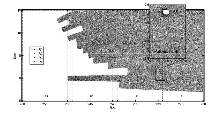
Figure 1: Distribution of all point sources with magnitude range $14\leq r\leq 22$ in the $40\times 20$ deg² area. This area are divided into four overlapped regions (R1, R2, R3 and R4) to be processed in batches because of too large number of objects. M5 (center: $\alpha=229.6\dg,\delta=2.1\dg$) and Palomar 5 (center: $\alpha=229.02\dg$, $\delta=-0.11\dg$) are two star-focus regions. The smaller box ($228.5\dg<\alpha<230.5\dg,-0.5\dg<\delta<2.5\dg$) encloses these two objects and the bigger one (subplot) shows the magnified image of the smaller one. The blank areas are regions which may be very dense clusters or bright stars or the regions the SDSS hasn’t covered.

Fig. 2 presents the interstellar extinction distribution derived based on the values of $E(B-V)$ from Schlegel et al. (1998). The resolution of the distribution is about 6 arcmin. There is smaller extinction in the northwest of the sky, but larger extinction in the southeast on the whole. The reddening correction in magnitude ($E(B-V)$) is 0.057 in average, and the maximum and minimum is about 0.384 and 0.016, respectively. All the sources in the sample are dereddened.

11

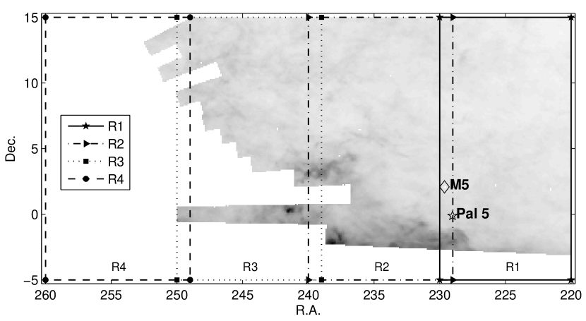
Figure 2: Distribution of interstellar extinction from the Milk Way. The resolution of this image is 6 arcmin, and E(B-V)s used by the SDSS databse are derived from Schlegel et al. (1998). As mentioned previously, the blank regions are M5, bright stars and areas not observed by the SDSS.

Following Belokurov et al. (2006), the difference between the magnitudes obtained by PSF photometry and by fitting an exponential profile, namely, $r_{\textrm{psf}}-r_{\textrm{exp}}$ distributions of both star and galaxy are plotted in Fig. 3. It is clear that stars are tightly concentrated around zero, whereas galaxies reveal a significant positive excess. Except for the cases mentioned in the previous section, classification is unauthentic when galaxies are point-like. PSF is the best fit model to estimate the magnitude of a point source ($r_{\textrm{psf}}$), while exponential model is one of models to calculate the magnitude of an extended one ($r_{\textrm{exp}}$). SDSS constructs a simple classifier with the analogous difference between $r_{\textrm{psf}}$ and ${r_{\textrm{exp}}}$. In Fig. 3, $r_{\textrm{psf}}-{r_{\textrm{exp}}}$ is concentrated on zero for point-like sources, while it is far away from zero for extended sources. Both of them have an intersection where stars and galaxies cannot be distinguished. Also following Belokurov et al. (2006), we take an threshold $r_{\textrm{psf}}-{r_{\textrm{exp}}}=0.05$ as the division between stars and galaxies. As a result, a sample of 4,082,662 point sources remains, which includes 1,079,301 in R1, 1,478,788 in R2, 1,378,560 in R3 and 146,013 in R4.

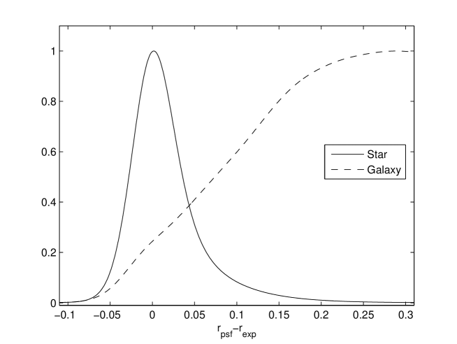
Figure 3: The distribution diagrams of $r_{\textrm{psf}}-r_{\textrm{exp}}$ for both star and galaxy. Kernel density estimation is used to fit the distributions with normal kernel and 0.02 bandwidth(Bowman et al., 1997). The two distributions are normalized to the peak value.

3 Back Propagation Neural Network

BPNN is now applied to various areas including astronomy, such as pattern classification, face and speech recognition and finance (Hangan, Demuth & Beale, 1996; Haykin, 1998). In astronomy, BPNN is used as classifier in both photometric and spectral aspects (von Hippel et al., 1994; Folkes et al., 1996) or morphological recognizer (Odewahn et al., 1992; Naim et al., 1995) in imaging or value estimator (Bailer-Jones, 2000) in determining theoretical models and physical parameters. Virtually, the specifical mechanism of BPNN is as follow: first, provide a train-test data set and train the configured BPNN with them, just as a teacher teaches a student to tell him which is a cluster star and which is a field one; then the BPNN learns the knowledge again and again to modify its inner configuration and makes itself perform well. During the course, BPNN will be judged by test data with the learned prior knowledge; at last, through this kind of repeated train-test-modify cycles, the classifier (BPNN) gains the features and has the best-learned experience to challenge new things. A data processing tool matlab, which provides a special neural network toolbox to design and realize all kinds of ANNs, is introduced in our work. The definition of neural networks, and other technical terms as well as the specified process of BPNN are described in the appendix.

As mentioned previously, Belokurov et al. (2006) used neural networks to reconstruct the probability distribution of cluster stars with the SDSS $ugriz$ photometric data. The idea of the approach is very simple: with $ugriz$ 5-band photometric data of cluster members and field stars as inputs of a BPNN, we get an estimation of the probability of cluster member as the output after the network is best trained. This method makes full use of photometric information and constructs a probability estimator in high dimensional data space with limited resources. When being trained, the BPNN can pick out bad sources automatically to form an accurate separator.

With the sample picked out strictly, the first step to detect the tidal tails is to figure out all the cluster members of Palomar 5 in the selected field. A lot of pattern recognition techniques are available, such as Bayes classifier, template matching, clustering analysis and artificial neural networks (see, e.g., Sergios & Konstantinos 2006, and references therein). In present study, the only thing we need to do is to estimate the membership probability of an object. BPNN can measure the posterior probability $P(C|\textbf{\emph{x}})$ in high dimension space, where $C$ denotes the cluster member class and x is the photometric data vector.

At last, we make a summary of the basic parameters and components of BPNN used in our paper. First, the dimension of input layer is 5 (photometric magnitudes) , and the transfer function of each neuron is Log-Sigmoid function. Then, the dimension of output vector is one, which yields 0 (for field stars) or 1 (for cluster stars). Mean squared error (MSE) is used to calculate the deviations between the output of BPNN and the real object type value. Finally, the Levenberg-Marquardt Backprogation (LMBP) algorithm is used to train the network to minimize the performance function MSE. The initial state (such as initial weights and biases, condition of termination, parameters of LMBP algorithm) is given automatically by matlab.

4 Tidal Tails Detection Based on BPNN

4.1 Data Set Selection for Training and Test

In order to apply the BPNN method to the tidal tails detection of Palomar 5, first of all, a training and test data set should be chosen to guide the BPNN to learn the knowledge of the cluster, so that it has the ability to figure out the probability of cluster member. As Belokurov et al. (2006) suggested, we select cluster stars from candidates using color-magnitude diagrams.

Along the main-sequence in the CMD, stars around the center of a cluster within a proper radius are likely to be members. Fig. 4 shows the radial number density distribution of stars around Palomar 5. We can see that the density descends from the center to the external of the cluster. As $R>0.25\dg$, the average number density becomes about $1.0958\pm 0.0497\times 10^{4}$ deg^-2. Radius $R$ = $0.13\dg$, where the density is a little higher than the average to avoid excessive field stars, is used to select candidates of cluster stars. About 1523 cluster member candidates are reserved.

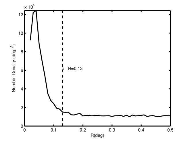
Figure 4: The radial number density distribution around the center of Palomar 5. The solid line shows that the density declines as the radius increases. The dashed line gives a threshold $R$ = 0.13$\dg$. Stars within the threshold radius are considered as cluster member candidates.

The next step is to pick out the most probable cluster stars from the 1523 candidates. Fig. 5 demonstrates the process of selecting cluster stars as a part of the training and test data set. Objects are reserved by encircling the CMD of $r$ vs $r-i$ (Fig. 5a) and $g$ vs $g-r$(Fig. 5b) with proper enclosures. These objects may be main-sequence stars, red giants and blue horizontal branch stars belonging to Palomar 5. In this way, contaminations from remanent galaxies and field stars (crosses in both CMDs) are almost eliminated. By intersection of these two CMDs, 957 objects are kept down to form the distribution of cluster stars in Fig. 5d (bigger black dots).

For field-star selection, $R>1\dg$, which is far enough from the center of Palomar 5, is adopted to choose candidates of field stars. Because the number of candidates is tremendous, it’s impossible to preserve all of them as our data set. Ideally, we hope that roughly equal numbers of objects should lie in both sides of the boundary in the data space so that they can fully represent these two classes. Accordingly, we chose field stars randomly in the sky, satisfying roughly equal numbers of both field and cluster stars near the main-sequence turnoff in the CMD. Thus, a box (a white rectangle with 4 hollow circles at the vertexes in Fig. 5d)with $19.5\leq r\leq 21$ and $0.05\leq r-i\leq 0.18$ is designed to form a region encircling the turnoff. There are about 320 stars in the box of the CMD for the cluster and field, respectively. As a result, 6991 field stars (smaller dots in Fig. 5c) and 957 cluster stars constitute the whole train-test data set (Fig. 5d). As mentioned previously, these field stars with target value 0 and cluster stars with value 1 are transmitted to train a BPNN. The BPNN will configure itself to estimate the possibility of cluster member for each object. Although the remained data set may contain impurities more or less, they are negligible relative to the total group sizes. And at the same time, BPNN will get rid of them automatically through being trained again and again, which is one of the reasons why we consider BPNN as our method.

(a)

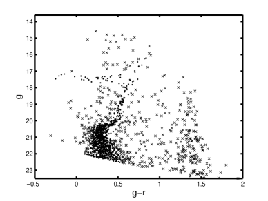
(b)

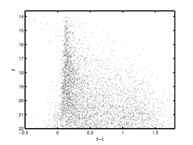
(c)

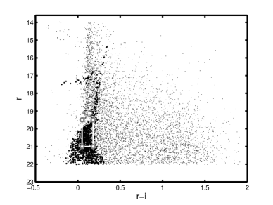
(d)

Figure 5: The color-magnitude diagrams used to select cluster and field stars. a) The CMD of $r$ vs $r-i$. Bold dots are the possible cluster members and crossings denote the excluded non-cluster sources. b) The CMD of $g$ vs $g-r$, used to assist $r$ vs $r-i$ CMD to pick out cluster stars from candidates. c) The distribution of the selected field stars in $r$ vs $r-i$ CDM. d) The $r$ vs $r-i$ CMD, including both the extracted cluster members and field stars. The smaller dots are field stars and the larger dots are cluster members. The white box with four circles shows the enclosure to decide the number of field star samples.

4.2 Network Structure Determination

In order to normalize the input data, we subtract the mean magnitudes of all data and then divide them by their standard deviations. Furthermore, for the sake of determining the number of layers and neurons in each layer, the star sample is segmented into training and test data sets. Training set is used to train a BPNN, while test set is used to measure its performance. Since cluster stars are relatively scarce, all of them are placed into the training set. Half field stars are laid aside stochastically into training data set and the others are regarded as test set.

Ten experiments are implemented for each designed BPNN to calculate the average output as the probability of cluster member. In this way, some random influences from initial weights, direction of modifying weights and algorithm terminating conditions are weakened. Here, one hidden layer and two hidden layers with 1, 10, 20, 30 and 40 neurons in the specified networks are investigated. The performance of them is showed in Fig. 6. Each network is trained and tested ten times with data set gained in the previous section. We stop the algorithm in every concerned network when the test MSE reaches its minimum. As Fig.6 indicates, with the increasing complication of network configuration, the training and test MSEs descend as a whole. And in the same network group (for example Layer 1 = 10), the test MSE always descends at first and then ascends when the number of neurons in the second hidden layer increases. No larger difference among the BPNNs with 2 hidden layers when the number of neurons in the first hidden layer is lager than 10. Considering about the test performance and the complexity of the configuration relevant to the speed of training, Net[5:10,10,1], which has 5 input elements, 10 neurons in the first hidden layer, 10 in the second hidden layer and 1 output, serves as our final model.

11 f6.eps

Figure 6: The mean training and test MSEs of various networks including 1 or 2 hidden layers. The darker solid line shows the training MSEs, while the light dotted line shows the test MSEs. The dashed horizontal line (MSE = 0.055) presents one level so that it can help us to check the network with the best performance.

4.3 Detect Tidal Tails With the Best Trained Network

It’s necessary to take into account the effectiveness of the trained networks. So, we construct a function of the magnitude ($r_{\textrm{psf}}$) as the ratio of the mean output for field and cluster stars in the training and test data set. Ideally, the ratio should be around zero as long as the networks are trained well. In Fig. 7, the ratio goes up gradually when $r_{\textrm{psf}}$ becomes fainter. No significant deviation is shown above 0.1 near the magnitude limit. This indicates that the selection of the training and test data set, and BPNNs are determined considerably well. However, in order to trace out the profile of the tidal tails more evidently, we cut off all the sources with a truncation $r_{\textrm{psf}}$ = 21 with smaller photometric errors.

Figure 7: The relation between the ratio of mean outputs for field and cluster stars and the $r_{\textrm{psf}}$ magnitude.

All the sources with normalized $ugriz$ magnitudes are imported into the trained ten networks, and the mean probability of cluster member for each star from the output layer is calculated. In order to present the panorama of the distribution of cluster stars, we divide the whole field into small square bins, whose sizes are $6^{\prime}\times 6^{\prime}$. About 90 objects are included in each bin, which is enough for statistical analysis. Here, the mean probability in each bin is computed. At the same time, Gaussian smoothing and median filtering are used to get rid of noises when detecting the tails in the field. In addition, in order to enhance the resolution of the distribution, cubic spline interpolation is also employed.

A lot of experiments are implemented to investigate the factors impacting the distribution. These tests include the parameters used in smoothing tools, the selection of cluster stars and the field stars chosen in different regions of the field. As a result, cluster stars within the radius $R<0.13\dg$ are appropriate for training the networks. Larger $R$ will bring in pollution from field stars, while smaller $R$ yields less cluster stars which cannot provide enough information about Palomar 5 members. Thus, the selection criterion of cluster stellar candidates in $\S$ 4.1 is reasonable. Field stellar samples chosen from different regions make no difference unless they cover the possible position of tidal tails. However, it does not affect the detection of the rest parts.

Fig. 8 exhibits the contours of 2-dimension probability distribution, where four regions are processed by the same best trained network and smoothing techniques. Although smoothed, the distribution is fluctuant in the whole field. We find the $P(C)s$, the probability of cluster member in all bins, obey a Gaussian distribution with mean value 0.0488 and standard deviation $\sigma$ = 0.0087. In order to check the tails more widely and to find possible longer tails, the contour levels are larger than $1\sigma$ above the mean. In this figure, M5 is detected at the same time, due to the similarity of their color-magnitude diagrams. The black solid line traveling through R2 and R3 provides us with a possible tidal tail away from the main tails in R0 ($226\dg<\alpha<236\dg$ and $-3\dg<\delta<5\dg$). We are not sure that the tail along this line is the real extension of the tails of Palomar 5, because the foreground noises in the residual regions are so similar to it. Fig. 9 shows the contours of the probability distribution, where the contour levels are higher than $1.5\sigma$ above the mean. The possible extension vanishes, but some debris still coexist with foreground noises. However, Grillmair & Dionatos (2006) insists that the extension is the real tail. Therefore, only the region R0, which encloses the clear tidal tails of Palomar 5, is considered as our region of investigation in the next discussion. The sub-figure in Fig. 9 shows the smoothed probability distribution with $1.5\sigma$ in R0. There are some ignorable differences between the two plots. These petty changes are caused by different bin coordinates and by region smoothing.

11 f8.eps

Figure 8: The contours of the smoothed probability distribution of cluster member with $1\sigma$ high above the mean. The solid line shows the possible extension, and dashed rectangle R0 is the target region we will discuss. The overlapped grey background is the reddening distribution of the Galaxy.

11 f9.eps

Figure 9: The contours of the smoothed probability distribution of cluster member with $1.5\sigma$ higher above the mean. The upper-right plot shows the recomputed distribution in the region R0. Detailed specifications should be referred to the text.

5 Properties of The Tidal Tails and The Cluster

5.1 The Profiles of the Tails

The subplot in Fig. 9 presents the holistic smoothed distribution of Palomar 5 members. The whole tail lies away from the dense regions of the Galactic extinction, which implies that the extinction has little effect on our detection. Two tails extend from the core region of Palomar 5 to southwest and northeast directions, which we called South Tail (ST) and North Tail (NT), respectively. ST is the leading part facing toward the Galactic disk, while NT is the trailing part. The angular distances are $5.42\dg$ for NT and $3.77\dg$ for ST. NT is a little shorter than the $5.8\dg$ northern tail detected by Odenkirchen et al. (2003), while the lengths of both ST are approximately equal. One reason may be that the smoothing flatten the distribution. In addition, the longer debris along the north tail detected by Odenkirchen et al. (2003) may be the disturbance or noise of field stars. However, the main tails we find are very similar to the results of Odenkirchen et al. (2003), while we do not support the discovery of any longer tails to the north of the sky that Grillmair & Dionatos (2006) reported to be a 22$\dg$ tail of Palomar 5, because the more extensive debris is so semblable to the background noises. There is no photometric data in the south, so we cannot cover larger southern regions to make sure a longer ST.

Another fact we can see from the contour map in Fig. 9 is that the distribution of cluster members is more dense in NT than that in ST. The possible reason causing this situation may be that: the orbit direction of NT is nearer to us than ST; given that the components of both tails are the same, because of their large extension, the average magnitude of NT ought to be brighter than that in ST. So, due to detecting limit, quite a few cluster members in ST cannot be observed or excluded by data preprocessing, although they are detected. However, when investigating all the detected members in both NT and ST, we do not find any large magnitude shift by comparing the mean magnitudes of the two tails in any places having the same distance from the cluster center. The maximum magnitude difference (between the northeast and southwest ends) is about 0.1 mag (NT is a little brighter than ST). Qualitative analysis indicates that even if the inclination angle of the tails is large, the magnitude difference is small when considering a specified star lying in different position in the tails. The above fact tells that it may be true that the track of NT is nearer to us, but it cannot change the distinct density difference of both tails obviously. Therefore, this kind of situation should be referred to some dynamical processes, which will be studied in future.

We convert the probability distribution to surface density distribution. First, we count the numbers of stars in all square bins. Then, the areas of all bins are calculated. In this way, with the smoothed probabilities of cluster member, we get the smoothed surface density distribution. Fig. 10a gives the transformed surface density contour map which is interpolated by the technique of cubic spline interpolation. Fig. 10a indicates that there are no obvious changes compared with the probability distribution contours. Furthermore, the noises around the tails and M5 are gotten rid of from the map. From Fig. 10a, we can see that there is no geometrical symmetry between ST and NT, and it takes on an S shape near the center of Palomar 5. In fact, Dehnen et al. (2004) has illustrated this structure in their simulations. Fig. 10b shows the radial surface density profiles of both ST and NT. In Fig. 10b, the numerical values originate from the smoothed density. Thus the density is lower than the density profile along the tails discussed by Odenkirchen et al. (2003). Both of density profiles drop down quickly from the center of Palomar 5. However, it seems to be that the density of NT descends not so fast than the ST. In addition, the trailing tail seems to lag behind the leading tail, because the density of ST reaches its peak at $R$ = $1.7\dg$, while NT achieves its minimum. This phenomena can be slightly seen in Odenkirchen et al. (2003) when he discussed the radial profiles of both tails, although he did not mention it. We cannot explain what causes this phenomena yet, but it is an interesting result. Possibly, this kind of lag is closely relative to the evolution of the cluster and the interaction between Palomar 5 and the Galaxy. Moreover, several stellar clumps emerge in both tails to form substructures of the cluster. Some of them lie at around $R=0.90\dg$ ($229.62\dg$, $0.56\dg$), $2.57\dg$ ($230.94\dg$, $1.6\dg$), $3.28\dg$ ($231.56\dg$, $19.6\dg$) and $5.13\dg$ ($233.28\dg$, $2.76\dg$) in the north, and $1.72\dg$ ($227.8\dg$, $-1.32\dg$) and $3.50\dg$ ($226.5\dg$, $-2.54\dg$) in the south. Maybe this kind of substructures and the radial density profiles are formed by dynamical processes between the Palomar 5 and the Galaxy. One possible explanation may be as follow: Palomar 5 has experienced several encounters with the Galactic disk or bulge since its birth; its body was heated by dynamical shocks; then the cluster stars were accelerated, and gradually disrupted and extended along the moving direction; as a result, some stars with small mass might escape from the tails, and the residual ones constitute the substructures and waited for the next shock. In fact, Odenkirchen et al. (2003) has indicated that Palomar 5 will be totally destroyed after the next disk crossing within about 100 Myr.

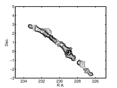
(a)

(b)

Figure 10: (a) The surface density contour map of Palomar 5, converted from the smoothed probability distribution map. Here, M5 and noises around the tails are erased. (b) The radial profiles of surface density (deg^-2) for both tails. The interval of the radial distance is 0.05.

5.2 King Model Fitting and the Luminosity Function

For density profile near the center, due to the small size of Palomar 5, we take $R<50^{\prime}$ as the range for discussion. Cluster stars are counted in all bins (from $2^{\prime}$ to $6.8^{\prime}$, the bin size is $0.3^{\prime}$; from $8^{\prime}$ to $15^{\prime}$, the bin size is $1^{\prime}$; the bin size of rest is $5^{\prime}$), and the area of each annulus is calculated. Fig. 11 shows the radial surface density profile, and the best fitting of King model (King, 1962). King model is expressed as:

$$\rho=k\left\{\frac{1}{\left[1+(R/r_{c})^{2}\right]^{\frac{1}{2}}}-\frac{1}{\left[1+(r_{t}/r_{c})^{2}\right]^{\frac{1}{2}}}\right\}^{2},$$ (1)

where $k$ is a constant, $r_{c}$ is the core radius, $r_{t}$ is the tidal radius and $R$ is the distance away from the center of the cluster. Thus, the centric density is

$$\rho_{0}=k\left\{1-\frac{1}{\left[1+(r_{t}/r_{c})^{2}\right]^{\frac{1}{2}}}\right\}^{2}.$$ (2)

$c=r_{t}/r_{c}$ is the concentration ratio. We fit the data subtracted from the background density (about 0.11) and obtain $k=114.9$, $r_{c}=1.60^{\prime}$, $r_{t}=14.29^{\prime}$. Therefore, the concentration ratio $c$ is 8.95 and $\rho_{0}$ is 90.81 arcmin^-2. We find that the radii obtained in this paper are smaller than those of Harris (1996): $r_{c}=3.25^{\prime}$ and $r_{t}=16.28^{\prime}$. From Fig. 11, we can see clearly that the King model cannot fit the observed profile at the outer regions ($R>8^{\prime}$) because of the tidal tails.

Figure 11: The radial surface distribution near the center of Palomar 5. The circles represent the surface densities in all bins figured out by counting the cluster stars. The King model with the mean background number density (0.11) is drawn in the solid line. The coordinate system is a logarithmic system and the unit of density is arcmin^-2.

Luminosity function (LF) of the cluster reflects its mass distribution. We examine whether the luminosity functions of the cluster itself and the tidal tails are the same, and try to verify that the tidal tails come from Palomar 5. We examine the luminosity functions in three regions: the north tail (N), the south tail (S1 $\&$ S2) and the Palomar 5 (C). Fig. 12a shows the boundaries of these regions. Radius $R=10^{\prime}$ is adopted for Palomar 5, and is near enough to the center of the cluster to eliminate the contamination from the tails. Radius $R>0.5\dg$, far enough away from the center, separates the tails into N for the north tail and S1 $\&$ S2 for the south tail. Star counts are taken to deduce the LFs of the ST and NT in these regions. We only consider the stars with high probability of cluster member ($>0.5$), which subsequently subtracts the contamination of foreground field stars. Consequently, in Fig. 12b, there are 4 LFs of ST, NT, total tails and the cluster itself, and all of them are rescaled to match the LF of the cluster. In the magnitude range of $19.0\leq r_{\textrm{psf}}\leq 20.0$, LFs are rescaled by factors 19.41, 22.43, 20.35 for NT, ST and total tails, respectively. On the whole, there is little difference among the LFs when $r_{psf}<20.5$. As $r_{psf}\geq 21$, the LF of the cluster lies lower than those of tails. This case confirms so-called ‘mass segregation effect’ (Koch et al., 2004), which shows that cluster members with big mass will accumulate near the center because of the loss of kinetic energy when colliding with others, while stars with small mass would escape from the cluster into its tails. Thus, these luminosity functions reveal the fact that the stars in the tails come from Palomar 5, and some relevant physical properties did not change much in its history.

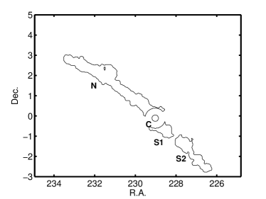
(a)

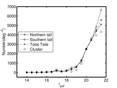
(b)

Figure 12: (a) The boundaries used to calculate the LFs. C is the boundary of cluster itself with $R<10^{\prime}$; N is the boundary of the north tail; S1+S2 is the boundary of the south tail. The boundaries of both NT and ST are far away from the center with $R>0.5\dg$. (b) Different luminosity functions. All LFs are rescaled by some factors to match the LF of the cluster.

6 conclusion

In this paper, we present a new method, Back Propagation Neural Network, to detect the tidal tails of globular cluster Palomar 5. Although some approaches such as matched-filter method (Rockosi et al., 2002) are widely applied to identifying the tails, we choose BPNN as our model to find the exact and distinct tails of Palomar 5. The photometric magnitudes of 5 bands ($ugriz$) in the SDSS DR6 are the unique inputs and consequently the probability of cluster member is the output in a best trained BPNN. BPNN resembles a black box, and we need not consider its detailed inner structure. The only thing we should do is to give it a set of well-selected cluster and field stars (they may not be completely accurate) as a teacher to make BPNN learn the knowledge. After gaining information, BPNN can estimate the probability of the cluster member.

First of all, we obtain about 15,305,060 objects in a $40\times 20$ deg² field ( $220\dg\leq\alpha\leq 260\dg$ and $-5\dg\leq\delta\leq 15\dg$). Considering the effectiveness of star/galaxy classification in the SDSS and the completeness of the observation, we leave behind about 4,082,662 point sources (stars) with $14\leq r_{\textrm{psf}}\leq 22$ after reddening correction and eliminating the pollution from galaxies as much as possible with the help of the distribution map of $r_{\textrm{psf}}-r_{\textrm{exp}}$. Next, we make use of surface density and CMDs to extract cluster stars from candidates, which lie in the circle where $R<0.13\dg$. And field stars used to be trained are chosen by making equal numbers of both cluster and field stars around the turnoff of main-sequence of Palomar 5. In this way, about 960 cluster stars and 6800 field stars are kept aside as the training and test data set to provide their inherent characteristic information for BPNN. With the training and test data, the best parameters and structures of BPNN are determined. Then the best trained BPNN with 5 nodes in the input layer, 10 neurons in the first hidden layer, 10 neurons in the second hidden layer and 1 neuron as output, is gained to compute the probability estimation of cluster member for each point source. We divide the field into bins with size $6^{\prime}\times 6^{\prime}$ to calculate the mean probability distribution. The impact of the selection of field stars is also investigated and their effect is not important.

S-shape tidal tails are detected, which subtend towards northeast and southwest from the center of the cluster: the trailing tail and the leading tail, respectively. The angular distances are $5.42\dg$ for the north tail and $3.77\dg$ for the south one. At the same time, there are some density clumps as the substructures of Palomar 5 in both tails. We cannot find any longer stretch for the NT if we do not regard the extension far away as tails, and we cannot confirm whether the ST has a longer spread because no photometric data are available outside to the southwest. We also find an interesting phenomenon from the radial profile of the density: the NT seems to lag behind the ST like wave propagation, which may be caused by the tidal shocks when Palomar 5 crossed the Galactic disk or bugle in its history. In addition, we fit the radial density profile near the cluster center with the King model and find that the model can fit this kind of remote globular clusters with low density very well when the radial distance is less than $8^{\prime}$. However, when the radial distance becomes larger, the density drops more slowly due to the tidal tails. The tidal radius obtained in this paper is $14.29^{\prime}$ and the core radius is $1.68^{\prime}$. Luminosity functions of both tails and the cluster are also determined. We find that there is little difference among the LFs of both tails coming from the original cluster, and their properties have not changed evidently during their lives.

Appendix A The Mechanism of BPNN

For clarity and continuity of our work, a BPNN with two hidden layers is demonstrated below (Fig. 13). This network contains input layer ($I$ in the figure), hidden layers ($L1$ and $L2$) and output layer ($O$) generally. Input layer reads training or test patterns (input patterns), which are offered to be processed by hidden layers and output layer yields the relevant output results. In our paper, input patterns are corresponding to 5-band magnitudes of cluster and field stars. The desired output patterns (target patterns) placed at $T$ in Fig. 13 are 1 for cluster stars or 0 for field ones. The output of BPNN gives the probability of cluster member for each star.

The network is executed in two phases: training phase and test phase. In training phase, input and target patterns are submitted to the network. And then two processes, feeding forward and error back propagation, are performed. After we endow this network with an initial state, an input sample (pattern) travels from the input layer. Via being treated by intermediate layers, the information stored by weights is processed and a corresponding result comes forth at the output layer. There, comparing the network output result with the relevant target pattern, an error performance is calculated. By this error item, error back propagation is carried out from output to input layer to modify the connected weights and biases (in Fig. 13), and store learned knowledge at the same time. Then, the remain patterns act in the same way and the iteration goes on until the satisfaction of preplanned error limit. There are two modes of updating weights and biases: one is incremental mode in which the weights and biases update when the errors of patterns back-propagate one by one as presented above and the other is batch mode in which all patterns travel through the network and the total error is counted, then the weights and biases are renewed once in an iteration. We call an iteration of processing all patterns as one ’epoch’. In test phase, patterns, which have not been seen by the network, are given to check the efficiency and accuracy of the network configured in training phase.

The detailed description of the network configuration and concise mathematics of training it are presented below. In the left panel of Fig.13, the input layer and target segment are divided by dashed lines, which are linked to exoteric environment. The nodes in the hidden and output layers are called neurons. The right panel of Fig.13 gives the delicate structure of one neuron. There are $p$ neurons from the previous layer as inputs connecting to the neuron enclosed by a dashed rectangle, where each connection has a weight $w$. In the neuron, an adder $\sum$ performs to sum all the input values and bias $\theta$ and transmits the result $v$ to a transfer function $f$, which is to produce an output $y$. Expressions can be presented as

$$v = \sum_{i=1}^{p}w_{i}x_{i}-\theta=\textbf{{w}}^{\prime}\textbf{{x}}-\theta,$$ (3)

$$y = f(v),$$ (4)

where $x_{i}$ is the output of the $i{\rm th}$ node from the previous layer and $w_{i}$ is the corresponding weight, and $\textbf{{x}}=[x_{1},x_{2},\ldots,x_{p}]^{\prime},\textbf{{w}}=[w_{1},w_{2},\ldots,w_{p}]^{\prime}$. More vividly to say, the stimulus $v$ goes beyond the bias ($\theta$), the neuron will be activated to release an output signal to next neurons. Here, $\theta$ can be arranged into the weight vector w, as long as we take into account another constant input of the node. That is to say, we introduce $x_{0}=-1$ and $w_{0}=\theta$ and let the network adjust $\theta$ just like weights, so that $v$ has the form of $v=\textit{{w}}^{\prime}\textbf{{x}}$, where $\textit{{x}}=[x_{0},x_{1},\ldots,x_{p}]^{\prime},\textit{{w}}=[w_{0},w_{1},\ldots,w_{p}]^{\prime}$. Besides, the transfer function $f$ has various forms, such as:

Linear: $$f =v,$$ (5)

Log-sigmoid: $$f =\frac{1}{1+e^{-v}},$$ (6)

Tan-sigmoid: $$f =\frac{2}{1+e^{-2v}}-1,$$ (7)

where $-\infty<v<+\infty$. Among these functions, the log-sigmoid transfer function, which yields results in the range from 0 to 1, is commonly used in back-propagation networks partly because of its unlimited differentiability. We will adopt this kind of transfer functions (Equation 6) in our present study.

fA1a.eps fA1b.eps

Figure 13: Left: A multilayer feed-forward back propagation network with 2 hidden layers. Right: A detailed model of one neuron in BPNN.

Now, turn back to training the network. We will select the batch training mode in this paper. In this mode, weights and bias will be updated only after the entire inputs and targets are submitted, and as a result, the gradients (quantitative changes of weights and bias) are averaged together to produce more accurate estimates. In this case, a performance function known as mean squared error is used to evaluate the outputs of the network. The MSE is expressed as a formula

$$E(\textit{{w}})=\frac{1}{N}\sum_{i=1}^{h}(T_{i}-O_{i})^{2}=\frac{1}{N}(\textbf{T}-\textbf{O})^{\prime}(\textbf{T}-\textbf{O})=\frac{1}{N}\|\textbf{T}-\textbf{O}\|^{2},$$ (8)

where $N$ is the numbers of input-target pairs, $h$ is the dimension of output vector O, T is the target pattern vector, $O_{i}$ and $T_{i}$ are the components of O and T, and w contains all the weights and bias in the BPNN. Additionally, target patterns are 1 or 0. Only one output neuron is needed, so $h=1$ in this paper.

Given the performance function, a training algorithm should be provided to teach the BPNN to learn how to classify. During training, our aim is to make the outputs approach the target patterns as much as possible, resulting in decreasing the value of MSE. That is, in order to adjust weights for better learning, we need to decrease the value of MSE or to minimize this performance function epoch by epoch. Consequently, an universal training scheme to update w comes up as

$$\triangle\textit{{w}}^{(k)}=\textit{{w}}^{(k+1)}-\textit{{w}}^{(k)}=\eta^{(k)}\textit{{d}}^{(k)}$$ (9)

or

$$\textit{{w}}^{(k+1)}=\textit{{w}}^{(k)}+\eta^{(k)}\textit{{d}}^{(k)},$$ (10)

where $k$ denotes the ${k_{th}}$ epoch of training, the positive $\eta$ is the learning rate which decides the step length of changes of w, and d is the search direction where w moves. All the training algorithms of back propagation network are variations of the above form. For example, the most basic algorithm, Steepest Descent BP (SDBP), is based on the negative gradient of $E(\textit{{w}})$ as d. Thus, the learning rule becomes

$$\triangle\textit{{w}}^{(k)}=-\eta^{(k)}\nabla{E(\textit{{w}})}\mid_{\textit{{w}}=\textit{{w}}^{(k)}},$$ (11)

where $\nabla{E(\textit{{w}})}$ is the differential of $E$. In this training algorithm, the detailed modifying formula of w in each layer is obtained by chain rule (Hangan, Demuth & Beale, 1996; Haykin, 1998, $\S$ 11.9), and relative learning rate can be optimized (Hangan, Demuth & Beale, 1996, $\S$ 9.6 & 12.12). There are other training algorithms to train BPNN: Backpropagation with Momentum (MOBP) (Hangan, Demuth & Beale, 1996, $\S$ 12.9), Conjugate Gradient Backpropagation (CGBP) (Hangan, Demuth & Beale, 1996, $\S$ 9.15 & 12.15), Newton Method using the Hessian matrix (second derivatives) of the performance as direction (Hangan, Demuth & Beale, 1996, $\S$ 9.10), Levenberg-Marquardt Backprogation (LMBP) (Hangan, Demuth & Beale, 1996, $\S$ 12.19) and so on. Here, we chose LMBP as our training algorithm because of its speediest convergence. Detailed algorithm about LMBP can also be referred to Ball et al. (2004).

References

- Abazajian et al. (2004) Abazajian, K., et al., 2004, AJ, 128, 502
- Adelman-McCarthy et al. (2008) Adelman-McCarthy, J. K., et al., 2008, ApJS, 175, 297
- Bailer-Jones (2000) Bailer-Jones, C. A. L., 2000, A&A, 357, 197
- Ball et al. (2004) Ball, N. M., Loveday, J.,Fukugita, M., Nakamura, O., Okamura, S., Brinkmann, J., & Brunner, R. J., 2004, MNRAS, 348, 1038
- Belokurov et al. (2006) Belokurov, V., Evans, N. W., Irwin, M. J., Hewett, P. C., & Wilkinson M. I., 2006, ApJ, 637, L29
- Bowman et al. (1997) Bowman, A. W., & Azzalini, A., 1997, Applied Smoothing Techniques for Data Analysis, New York: Oxford University Press
- Carney (1984) Carney, B. W., 1984, PASP, 96, 841
- Folkes et al. (1996) Folkes, S. R., Lahav, O., & Maddox, S. J., 1996, MNRAS, 283, 651
- Dehnen et al. (2004) Dehnen, W., Odenkirchen, M., Grebel, E. K., & Rix, H.-W., 2004, AJ, 127, 2753
- Grillmair et al. (1995) Grillmair, C. J., Freeman, K. C., Irwin, M., & Quinn, P. J., 1995, AJ, 109, 2553
- Grillmair & Johnson (2006) Grillmair, C. J., & Johnson, R., 2006, ApJ, 639, L17
- Grillmair & Dionatos (2006) Grillmair, C. J., & Dionatos O., 2006, ApJ, 641, L37
- Hangan, Demuth & Beale (1996) Hangan, M. T., Demuth, H. B., & Beale, M. H., 1996, Neural Network Design, Boston, MA: PWS Publishing
- Harris (1996) Harris, W. E., 1996, AJ, 112, 1487
- Haykin (1998) Haykin, S., 1998, Neural Networks: A Comprehensive Foundation, 2nd Edition, Harlow, En:Prentice Hall
- King (1962) King, I., 1962, AJ, 67, 471
- Koch et al. (2004) Koch, A., Grebel, E. K., Odenkirchen, M., Martínez-Delgado, D., & Caldwell, J. A. R., 2004, AJ, 128, 2274
- Lauchner et al. (2006) Lauchner, A., Powell JR, W. L., & Wilhelm, R., 2006, ApJ, 651, L33
- Leon et al. (2000) Leon, S., Meylan, G., & Combes, F., 2000, A&A, 359, 907
- Lupton et al. (2001) Lupton, R., Gunn, J. E., Ivezić, Z., Knapp, G. R., & Kent, S., 2001, Astronomical Data Analysis Software and Systems X, 238, 269
- Naim et al. (1995) Naim, A., et al., 1995, MNRAS, 274, 1107
- Odewahn et al. (1992) Odewahn, S. C., Stockwell, E. B., Pennington, R. L., Humphreys, R. M., & Zumach, W. A., 1992, AJ, 103, 318
- Odenkirchen et al. (2001) Odenkirche, M., et al., 2001, ApJ, 548, L165
- Odenkirchen et al. (2003) Odenkirche, M., et al., 2003, AJ, 126, 2385
- Rockosi et al. (2002) Rockosi, C. M., et al., 2002, AJ, 124, 349
- Schlegel et al. (1998) Schlegel, D. J., Finkbeiner, D. P., & Davis, M., 1998, ApJ, 500, 525
- Sergios T. et al. (2006) Sergios, T., & Konstantinos, K., 2006, Pattern Recognition, 3rd ed., Athens: Academic Press
- Smith et al. (1986) Smith, G. H., McClure, R. D., Stetson, P. B., Hesser, J. E., & Bell, R. A., 1986, AJ, 91, 842
- Spitzer (1987) Spitzer, L., 1987, Dynamical Evolution of Globular Clusters, Princeton, NJ: Princeton University Press
- Stoughton et al. (2002) Stoughton, C., et al., 2002, AJ, 123, 485
- von Hippel et al. (1994) von Hippel, T., Storrie-Lombardi, L. J., Storrie-Lombardi, M. C., & Irwin, M. J., 1994, MNRAS, 269, 97
- Wu et al. (2003) Wu, Z.-Y., Shu, C.-G., & Chen, W.-P., 2003, Chin.Phys.Lett., 20, 1648
- Wu et al. (2004) Wu, Z.-Y., Zhou, X., & Ma, J., 2004, Chin.Phys.Lett., 21, 418