General Polytropic Magnetofluid under Self-Gravity: Voids and Shocks

Abstract

We study the self-similar magnetohydrodynamics (MHD) of a quasi-spherical expanding void (viz. cavity or bubble) in the centre of a self-gravitating gas sphere with a general polytropic equation of state. We show various analytic asymptotic solutions near the void boundary in different parameter regimes and obtain the corresponding void solutions by extensive numerical explorations. We find novel void solutions of zero density on the void boundary. These new void solutions exist only in a general polytropic gas and feature shell-type density profiles. These void solutions, if not encountering the magnetosonic critical curve (MCC), generally approach the asymptotic expansion solution far from the central void with a velocity proportional to radial distance. We identify and examine free-expansion solutions, Einstein-de Sitter expansion solutions, and thermal-expansion solutions in three different parameter regimes. Under certain conditions, void solutions may cross the MCC either smoothly or by MHD shocks, and then merge into asymptotic solutions with finite velocity and density far from the centre. Our general polytropic MHD void solutions provide physical insight for void evolution, and may have astrophysical applications such as massive star collapses and explosions, shell-type supernova remnants and hot bubbles in the interstellar and intergalactic media, and planetary nebulae.

1 Introduction

Supernova explosions, planetary nebulae and stellar winds from massive stars are believed to be the main sources of creating voids (i.e. bubbles, cavities) in the interstellar medium (ISM) (e.g. Ferrière 1998, 2001 and extensive references therein). In the local ISM, the remnant of a typical isolated supernova grows for $\sim$ 1.5 Myr and reaches a maximum radius of $\sim 50$ pc. The shell-type supernova remnants (SNRs) appear quasi-spherical and the masses within them have been swept up by ejecta from supernovae. An example of such structure is a void region towards the Lupus dark cloud complex, which was revealed through observations of 100 $\mu$m emissions (e.g. Gahm et al. 1990; Franco 2002) soft X-ray (e.g. Riegler et al. 1980), and 21 cm HI line (e.g. Colomb et al. 1984). Neutral hydrogen (HI) voids have also been found in filled-centre SNRs (e.g. Wallace et al. 1994).

Voids may also emerge long before we actually observe SNRs. According to the neutrino-driven mechanism of type-II and type-Ibc supernova explosions (e.g. Janka & Hillebrant 1989; Janka & Müller 1995, 1996), within the first second of a type II supernova, the intense neutrino flux generated by the central core bounce heats the surrounding stellar mass and pushes the stellar material outwards. Subsequently, a rebound shock emerges and propagates outwards (e.g. Lou & Wang 2006, 2007; Hu & Lou 2009). After several hundred milliseconds, the neutrino-sphere decouples from the gas, and may leave behind a cavity around the centre during a supernova. After this decoupling, the exploding star with a central cavity continues to expand and the central cavity eventually evolves into a hot bubble in the ISM.

Massive stars can also create voids in the ISM through photoionization heating and stellar winds (e.g. Castor et al. 1975; Weaver et al. 1977; McKee et al. 1984). Likewise, fast winds from central compact hot white dwarfs may generate expanding cavities in planetary nebulae (e.g. Lou & Zhai 2009). HI voids and shells have been found and observed by radio observations around several Galactic Wolf-Rayet (WR) stars – massive stars undergoing significant mass losses (e.g. Cappa & Miemela 1984; Cappa et al. 1986, 1988; Dubner et al. 1990; Niemela & Cappa 1991; Arnal & Mirabel 1991; Arnal 1992). On larger scales, observations show that voids also exist in neutral hydrogen discs of spiral galaxies (e.g. Crosthwaite & Turner 2000). Recently, central cavities of $\sim 200$ kpc diameter and large-scale shock fronts have been revealed by Chandra X-ray observations in the galaxy cluster MS0735.6+7421 (e.g. McNamara et al. 2005).

The dynamic evolution of voids in the ISM still lacks a systematic theoretical exploration. Dyson & Williams (1997) provided qualitative description on the gas dynamic effects of massive stars on the ISM. Chevalier (1997) studied the expansion of a photoionized stellar wind in late stages of stellar evolution (e.g. supernovae and planetary nebulae; see also Meyer 1997). From the centre, a stellar system consists of a hot bubble of shocked fast wind, a region of shocked and photoionized wind, and an outer region of slow wind. Chevalier (1997) also employed the isothermal self-similar transformation as Shu (1977) but without gravity to model the self-similar dynamic evolution of an outer slow wind. Physically, the fast hot wind bubble resembles the concept of a central void of this paper. Hu & Lou (2008a) presented self-similar void solutions to model “champagne flows” of H II regions after the nascence of a massive protostar in a conventional polytropic gas. Such voids embedded in nebulae can be created and sustained by fast stellar winds and photoionization heating. Here, we formulate an MHD problem with a general polytropic gas under self-gravity.

The system of interest is a general polytropic magnetofluid with a quasi-spherical symmetry under self-gravity, thermal pressure gradient force and magnetic Lorentz force. We further find that MHD shocks are indispensable to establish sensible global solutions, for example with the asymptotic velocity at large radii tending to zero. Magnetic field can be extremely important in many astrophysical processes on different scales and in particular, for star formation activities at various stages (e.g. Shu et al. 1987; Myers 1998). The Crab Nebula is observed to be supported by the magnetized pulsar wind (e.g. Lou 1993; Wolf et al. 2003). When rotation is sufficiently slow in an astrophysical system, the overall geometry may remain quasi-spherical and the quasi-spherical random-field approximation (e.g. Zel’dovich & Novikov 1971) can be applicable. Chiueh & Chou (1994) discussed the gravitational collapse of an isothermal magnetized gas cloud by including the magnetic pressure force from a randomly distributed magnetic field. Recently, we have provided detailed analyses by assuming a random transverse magnetic field with the consideration of both magnetic pressure and tension forces (Yu & Lou 2005; Yu et al. 2006; Lou & Wang 2007; Wang & Lou 2007, 2008). We presume that the non-spherical flows as a result of the magnetic tension force may be neglected as compared to the large-scale mean radial bulk motion of gas. The key point is that the (self-)gravity is strong enough to hold on the entire gas mass and induce core collapse, or the driving force is strong enough to generate a quasi-spherical void. Therefore on large scales a completely random magnetic field contributes to the dynamics in the form of the average magnetic pressure gradient force and the average magnetic tension force in the radial direction. This approximation was discussed in more details by Wang & Lou (2007).

The general equation of state is $p=\kappa(r,\ t)\rho^{\gamma}$ where $p$ is the thermal gas pressure, $\rho$ is the mass density, $\gamma$ is the polytropic index and $\kappa$ is a proportional coefficient dependent on both radius $r$ and time $t$. For a global constant $\kappa$, the equation of state is that of a conventional polytropic gas (e.g. Suto & Silk 1988; Lou & Gao 2006; Lou & Wang 2006, 2007; Hu & Lou 2008a). By setting $\gamma=1$ and $\kappa$ as a global constant, a conventional polytropic gas then becomes an isothermal gas. In case of $\gamma>1.2$, novel quasi-static asymptotic solutions for a polytropic gas exist in approach to the system centre (see Lou & Wang 2006). As the specific enthalpy is $p/(\gamma-1)$, we thus require $\gamma\geq 1$ to ensure a positive specific enthalpy. A general polytropic gas features the conservation of specific entropy along streamlines. The conventional polytropic case is a only special case with constant specific entropy everywhere at all times. A general polytropic model with random magnetic field is the most general model of a polytropic magnetofluid of quasi-spherical symmetry under self-gravity (Wang & Lou 2008; Jiang & Lou 2009).

Our self-similar transformation employs a dimensionless independent similarity variable $x$ defined as a combination of radius $r$ and time $t$ such that $x=r/(k^{1/2}t^{n})$ where $k$ is the so-called ‘sound parameter’ to make $x$ dimensionless and $n$ is a key scaling index. Theoretically, our void solutions are those solutions whose enclosed mass is zero within a certain radius denoted as $x^{*}$. This radius expands with time in a self-similar manner, i.e. $r^{*}=k^{1/2}x^{*}t^{n}$. By this expression, the physical meaning of the self-similar scaling index parameter $n$ is evident. The expansion speed of the void boundary is $u^{*}\propto t^{(n-1)}$; therefore for $n>1$, a void expands faster and faster (i.e. acceleration), while for $n<1$, a void expands slower and slower (i.e. deceleration); and for $n=1$, a void expands at a constant speed. The void boundary may also be regarded as an idealization of a contact discontinuity between a faster wind and a slower winds (e.g. Chevalier 1997; Lou & Zhai 2009).

The case of $\gamma=4/3$ corresponds to a relativistically hot gas that deserves a special attention. Homologous core collapse for a relativistically hot gas was studied by Goldreich & Weber (1980) and the behaviour of such system has been treated by Yahil (1983) as a limit of $\gamma\rightarrow(4/3)^{+}$. Recently, Lou & Cao (2008) presented an illustrative example of void in such a system. In this paper, we study voids for a magnetized Newtonian gas (i.e. $\gamma\neq 4/3$ in general), as well as voids in a relativistically hot fluid (i.e. $\gamma=4/3$), and we offer several concrete examples.

This paper is structured as follows. Section 1 is an introduction to provide background information and the motivation of this investigation; Section 2 describes first the formulation of a general polytropic magnetofluid under quasi-spherical symmetry, and secondly analytic asymptotic solution behaviours near the void boundary in various parameter regimes, and thirdly various asymptotic MHD solutions that are useful in constructing global semi-complete solutions (i.e. solutions that are valid in the range $0<x<+\infty$); Section 3 describes and discusses properties of void solutions with different parameters, in contexts of hydrodynamics and MHD, and presents a few examples; Section 4 gives examples of astrophysical applications of such void solutions. Finally, Section 5 contains conclusions and discussion. Mathematical derivations are included in an appendix.

2 Self-Similar MHD with Quasi-Spherical Symmetry

2.1 Formulation of a Nonlinear MHD Problem

The MHD evolution of a general polytropic gas of quasi-spherical symmetry and under self-gravity can be described by a set of nonlinear MHD partial differential equations (PDEs) in spherical polar coordinates $(r,\ \theta,\ \phi)$, namely

$$\frac{\partial\rho}{\partial t}+\frac{1}{r^{2}}\frac{\partial}{\partial r}(r^{2}\rho u)=0\ ,$$ (1)

$$\frac{\partial M}{\partial r}=4\pi r^{2}\rho\ ,$$ (2)

$$\rho\frac{\partial u}{\partial t}+\rho u\frac{\partial u}{\partial r}=-\frac{\partial p}{\partial r}-\frac{GM\rho}{r^{2}}-\frac{\partial}{\partial r}\frac{<B_{t}^{2}>}{8\pi}-\frac{<B_{t}^{2}>}{4\pi r}\ ,$$ (3)

where $\rho(r,\ t)$ is the mass density, $u(r,\ t)$ is the bulk radial gas flow speed, $M(r,\ t)$ is the enclosed mass within radius $r$ at time $t$, $p$ is the thermal gas pressure, $G=6.67\times 10^{-8}$ dyne cm² g^-2 is the gravitational constant, and $<B_{t}^{2}>$ is the ensemble average of a random transverse magnetic field squared (i.e. proportional to the magnetic energy density). Equations (1) and (2) represent mass conservation, leading to ${\partial M}/{\partial t}+u{\partial M}/{\partial r}=0$. We assume a random magnetic field mainly in transverse directions, and the magnetic force perpendicular to magnetic field lines directs to the radial direction and appears in the radial momentum equation (3) as the magnetic pressure and tension terms. Together with magnetic induction equation

$$\bigg{(}\frac{\partial}{\partial t}+u\frac{\partial}{\partial r}\bigg{)}(r^{2}<B_{t}^{2}>)+2r^{2}<B_{t}^{2}>\frac{\partial u}{\partial r}=0\$$ (4)

and the specific entropy conservation along streamlines

$$\bigg{(}\frac{\partial}{\partial t}+u\frac{\partial}{\partial r}\bigg{)}\bigg{(}\ln\frac{p}{\rho^{\gamma}}\bigg{)}=0\$$ (5)

with $\gamma$ being the polytropic index, we complete the model formulation for a general polytropic MHD with a quasi-spherical symmetry (Wang & Lou 2007, 2008).

In this paper, we consider self-similar solutions which form an important subclass of nonlinear MHD PDEs. In order to reduce these nonlinear MHD PDEs to self-similar ordinary differential equations (ODEs), we introduce the following self-similar transformation as Wang & Lou (2008), namely

$$\!\!\!\!\!\!\!\!\!r=k^{1/2}t^{n}x,\qquad u=k^{1/2}t^{n-1}v\ ,\qquad\quad\rho=\frac{\alpha}{4\pi Gt^{2}}\ ,\qquad$$

$$\!\!\!\!\!\!\!\!\!\!\!\!\!\!\!\!\!p=\frac{kt^{2n-4}}{4\pi G}\beta\ ,\quad M=\frac{k^{3/2}t^{3n-2}m}{(3n-2)G}\ ,\quad<B_{t}^{2}>=\frac{kt^{2n-4}w}{G},$$ (6)

where $v(x)$, $\alpha(x)$, $\beta(x)$, $m(x)$, $w(x)$ are dimensionless reduced variables of $x$ only. We refer to $v(x)$, $\alpha(x)$, $\beta(x)$, $m(x)$ and $w(x)$ as the reduced radial speed, mass density, thermal pressure, enclosed mass and magnetic energy density, respectively. Self-similar transformation (6) is identical with that of Wang & Lou (2007, 2008). By substituting self-similar transformation (6) into equations (1)$-$(5), we obtain several valuable integrals

$$w=h\alpha^{2}x^{2}\ ,$$ (7)

$$\beta=C\alpha^{\gamma}m^{q}\ ,$$ (8)

$$m=\alpha x^{2}(nx-v)\ .$$ (9)

Equation (7) corresponds to the frozen-in condition for magnetic field in the ideal MHD approximation, where $h\equiv<B_{t}^{2}>/(16\pi^{2}G\rho^{2}r^{2})$ is a dimensionless magnetic parameter representing the average strength of a random transverse magnetic field.

Equation (8) is the self-similar form of the specific entropy conservation along streamlines, where the exponent parameter $q\equiv 2(n+\gamma-2)/(3n-2)$ and thus $\gamma=2-n+(3n-2)q/2$, and $C$ is an arbitrary coefficient from integration. For $q=0$, the flow system involves a conventional polytropic gas with a constant specific entropy everywhere in space and at all times; for $q>0$, the specific entropy increases from inside (smaller $x$) to outside (larger $x$); and $q=2/3$ leads to $\gamma=4/3$ for a relativistically hot gas (e.g. a photon gas, a neutrino gas or an extremely high temperature electron gas) with an arbitrary $c$. Actually we may set $C=1$ in all cases with $q\neq 2/3$ without loss of generality, because an adjustment of sound parameter $k$ in self-similar transformation (6) to $C^{1/(1-3q/2)}k$ would make $C$ disappear.

Equation (9) requires both $3n-2>0$ and $nx-v>0$ for a positive enclosed mass $M(r,\ t)$. When $nx-v=0$ at a certain $x^{*}$, the enclosed mass vanishes by equation (9); this is referred to as a void with $x^{*}$ being the void boundary in a self-similar expansion. Accordingly, the reduced radial velocity on the boundary is given by $v^{*}=nx^{*}$. The condition $nx-v=0$ on the void boundary implies that the self-similar expansion speed of the void boundary $dr^{*}/dt$ is equal to the radial flow velocity on the void boundary $u(r^{*},t)$. This is regarded as the physical condition for a contact discontinuity between the outer slower stellar wind and the inner faster wind driving a hot bubble by Chevalier (1997) for $q=0$, $n=1$, $\gamma=1$ and without gravity. Lou & Zhai (2009) considered a gas dynamic model for planetary nebulae with contact discontinuities for an isothermal self-gravitating gas. From now on, we denote variables on the void boundary by a superscript asterisk ^∗.

Combining all equations above, we obtain coupled nonlinear MHD ODEs for the two first derivatives $\alpha^{\prime}$ and $v^{\prime}$ in the following compact forms of

$${\cal X}(x,\alpha,v)\alpha^{\prime}={\cal A}(x,\alpha,v)\ ,\qquad{\cal X}(x,\alpha,v)v^{\prime}={\cal V}(x,\alpha,v)\ ,$$ (10)

where the three functional coefficients ${\cal X}$, ${\cal A}$ and ${\cal V}$ are explicitly defined by

$$\!\!\!\!\!\!\!\!\!{\cal X}(x,\ \alpha,\ v)\equiv C\bigg{[}2-n+\frac{(3n-2)}{2}q\bigg{]}$$

$$\quad\times\alpha^{1-n+3nq/2}x^{2q}(nx-v)^{q}+h\alpha x^{2}-(nx-v)^{2}\ ,$$

$$\!\!\!\!\!\!\!\!\!{\cal A}(x,\ \alpha,\ v)\equiv 2\frac{x-v}{x}\alpha\big{[}Cq\alpha^{1-n+3nq/2}x^{2q}(nx-v)^{q-1}$$

$$\quad+(nx-v)\big{]}-\alpha\bigg{[}(n-1)v+\frac{(nx-v)}{(3n-2)}\alpha+2h\alpha x$$

$$\quad+Cq\alpha^{1-n+3nq/2}x^{2q-1}(nx-v)^{q-1}(3nx-2v)\bigg{]}\ ,$$

$$\!\!\!\!\!\!\!\!\!{\cal V}(x,\ \alpha,\ v)\equiv 2\frac{(x-v)}{x}\alpha\bigg{[}C\bigg{(}2-n+\frac{3n}{2}q\bigg{)}$$

$$\quad\times\alpha^{-n+3nq/2}x^{2q}(nx-v)^{q}+hx^{2}\bigg{]}$$

$$\quad-(nx-v)\bigg{[}(n-1)v+\frac{(nx-v)}{(3n-2)}\alpha+2h\alpha x$$

$$+Cq\alpha^{1-n+3nq/2}x^{2q-1}(nx-v)^{q-1}(3nx-2v)\bigg{]}\ .$$ (11)

The formulation above is largely the same as Wang & Lou (2008), except for an additional free parameter $C$ in cases with $q=2/3$ (i.e. $\gamma=4/3$). Wang & Lou (2008) also provides procedures to determine magnetosonic critical curve (MCC), eigensolutions across the MCC and MHD shock jump conditions across the magnetosonic singular surface (see Appendix A).

The MCC for $q=2/3$ and thus $\gamma=4/3$ is special. Extensive numerical explorations suggest that the MCC bears the simple form of $v=\eta x,\ \alpha=$ constant, where $\eta$ is a constant coefficient dependent on parameters $n,\ h$ and proportional factor $C$. Substituting this form into equation (11) and the MCC conditions ${\cal X}=0$ and ${\cal A}=0$ become respectively

$$\alpha=\frac{(n-\eta)^{2}}{h+({4}/{3})C(n-\eta)^{2/3}}\ ,$$ (12)

$$\frac{2}{3}C\alpha(n-\eta)^{-1/3}(2-3n)+2(1-\eta)(n-\eta)$$

$$\quad=(n-\eta)\eta+\frac{(n-\eta)}{(3n-2)}\alpha+2h\alpha\ .$$ (13)

Substituting relation (12) into equation (13) to eliminate $\alpha$, we immediately derive an expression for the constant coefficient $\eta$ in terms of $n,\ h$ and $C$. Once $\eta$ is known in relation (12), we can compute $\alpha$ value accordingly. With $h=0$, relations (12) and (13) give the same solution as discussed in Lou & Cao (2008) for a nonmagnetized relativistically hot gas. Here, we extend the special MCC with $\gamma=4/3$ to a magnetofluid embedded with a random transverse magnetic field.

2.2 Behaviours of a Polytropic Void Boundary

We now analyze asymptotic behaviours around the void boundary $x^{*}$, and these boundary conditions will be used to construct various solutions in numerical integrations starting from the void boundary.

The gas pressure should be continuous across the void boundary, otherwise a shrinkage of the void boundary with diffusions would be expected. According to equation (8) and for $\alpha\neq 0$, inequality $q<0$ on $nx^{*}-v=0$ leads to a diverging reduced pressure $\beta$. For $q\geq 0$, it follows automatically that $\beta=0$ at the void boundary. Therefore to ensure $\beta^{*}\equiv\beta(x^{*})=0$, we require $\alpha*\equiv\alpha(x^{*})=0$ in cases of $q<0$, or $\alpha^{*}\geq 0$ in cases of $q\geq 0$. It is favorable to further require the continuity of mass density, as a discontinuous density would lead to a local diffusion, in addition to a global self-similar evolution. Therefore, a solution with $\alpha=0$ at $nx^{*}-v=0$ is regarded as a physically sensible one, otherwise the self-similar solution should be seen as an asymptotic solution valid in the region sufficiently far from the void boundary.

2.2.1 Hydrodynamic and MHD Cases with $\alpha^{*}=0$
    on the Expanding Void Boundary

The void boundary obeying $\alpha=0$ and $nx-v=0$ may possibly become a critical curve with the three functional coefficients on both sides of equations (10) being zero. According to equation (11), the possible non-zero terms of the three functional coefficients ${\cal X}$, ${\cal A}$ and ${\cal V}$ approaching the void boundary $nx-v=0$ and $\alpha=0$ are the thermal pressure gradient force terms, namely

$${\cal X}\sim C\gamma x^{2q}\alpha^{\gamma+q-1}(nx-v)^{q}\ ,$$

$${\cal A}\sim C(2-3n)qx^{2q}\alpha^{\gamma+q}(nx-v)^{q-1}\ ,$$

$$\!\!\!\!\!\!\!\!\!\!\!\!\!\!{\cal V}\sim C[2(1-n)\gamma+(2-3n)q]x^{2q}\alpha^{\gamma+q-1}(nx-v)^{q}\ ,$$

(14)

where we have used the relation $\gamma=2-n+(3n-2)q/2$ .

According to expressions (14), the parameter regime of $q\geq 0\ ,\ \gamma+q\geq 1$, except for the special isothermal case ($q=0,\ \gamma+q=1$), ensures the vanishing of ${\cal X}$ and ${\cal V}$ on the void boundary; when $\alpha\sim(nx-v)$ near the void boundary as shown by our analysis presently, then ${\cal A}$ also vanishes at the void boundary, and the void boundary indeed becomes a MCC.

By a local first-order Taylor series expansion, we obtain from equations (10) and (11) two pairs of eigensolutions for the first derivatives of $v(x)$ and $\alpha(x)$ across the void boundary as a critical curve. The one that ensures positive enclosed mass is

$$v^{\prime}\mid_{x^{*}}=\Big{(}-2+2\sqrt{2}\Big{)}(n-1)\ ,$$

$$\alpha^{\prime}\mid_{x^{*}}=\sqrt{2}\bigg{[}\frac{(2-n)}{(3n-2)q}+\frac{1}{2}\bigg{]}(n-1)^{2}\frac{n}{hx^{*}}\ .$$ (15)

It can be shown that for $n\neq 1$, all points on this critical curve are saddle points (e.g. Jordan & Smith 1977). It is known that around a saddle singular point, only solutions along the direction defined by eigensolutions are allowed. Therefore for $\alpha^{*}=0$ at the void boundary, the self-similar solutions would follow the behaviour described by expression (15). The presence of magnetic field is crucial here. In a purely hydrodynamic case of $h=0$ or a conventional polytropic case of $q=0$, the reduced density gradient $\alpha^{\prime}$ diverges at the void boundary $x=x^{*}$. It would require additional considerations for a void boundary on which the mass density vanishes but its first derivative diverges. To better describe a sudden change of mass density on the void boundary, we would then set a non-zero mass density $\alpha^{*}\neq 0$ at the void boundary (see analyses in the following sections). The valid regime of parameters in which solution (15) stands is therefore $q>0,\ \gamma+q\geq 1$ and $h>0$. As we should further require $\gamma\geq 1$ for a positive enthalpy, the valid regime of parameters is simply $q>0$ and $h>0$.

If the three functional coefficients ${\cal X}$, ${\cal A}$ and ${\cal V}$ do not vanish at the void boundary, the leading terms of the first derivatives of $v$ and $\alpha$ at the void boundary are then

$$v^{\prime}\mid_{x^{*}}=2(1-n)+(2-3n)q/\gamma\ ,$$ (16)

$$\alpha^{\prime}\mid_{x^{*}}=\frac{(2-3n)q}{\gamma}\frac{\alpha}{(nx-v)}$$

$$\quad\quad=-\frac{q\alpha}{(\gamma+q)}(x-x^{*})^{-1}\ .$$ (17)

Note the coefficient $C$ disappears in these two expressions. The second equality for $\alpha^{\prime}$ in equation (2.2.1) involves equation (16). The asymptotic solution of $\alpha$ near the void boundary is

$$\alpha=K(x-x^{*})^{-q/(\gamma+q)}+\cdot\cdot\cdot\ ,$$ (18)

where $K$ is an arbitrary integration constant referred to as the void density parameter. To ensure solution (18) going to zero in the limit of $x\rightarrow x^{*}$, we require $q/(\gamma+q)<0$. We now verify that for such solutions, ${\cal X}$, ${\cal A}$ and ${\cal V}$ actually diverge at the void boundary. With solutions (16)$-$(18), we have ${\cal X}\sim(x-x^{*})^{q/(\gamma+q)}$, ${\cal V}\sim(x-x^{*})^{q/(\gamma+q)}$, ${\cal A}\sim(x-x^{*})^{-1}$. Therefore, the condition $q/(\gamma+q)<0$ in the meantime ensures the validity of the asymptotic solution. We should require $\gamma\geq 1$ as a physical requirement and thus inequality $q/(\gamma+q)<0$ is equivalent to $q<0$ and $\gamma+q>0$.

A positive enclosed mass requires $v^{\prime}\mid_{x^{*}}<n$, which provides a lower limit for the index $q$, namely

$$q>q_{\rm min}=\frac{4+3n^{2}-8n}{3n(3n/2-1)}=\frac{2(n-2)}{3n}\ ,$$ (19)

where $n-2<0$. With algebraic manipulations, it is proven that inequality (19) together with $\gamma\geq 1$ is equivalent to inequality $\gamma+q>0$. Thus within the parameter regime of $q<0$ and $\gamma+q>0$ where solutions $(\ref{CC1})-(\ref{CC3})$ stand, inequality $v^{\prime}\mid_{x^{*}}<n$ is automatically satisfied.

In summary, in the vicinity of the void boundary $nx-v=0$ with $\alpha=0$, we find two possible types of asymptotic solutions. The parameter regimes in which these solutions are applicable are shown in Figure 1 accordingly.

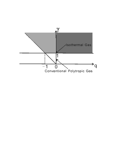
Figure 1: Regimes of parameters $q$ and $\gamma$ for which asymptotic solutions near the void boundary are applicable. The horizontal axis is the parameter $q$ and the vertical axis is the polytropic index $\gamma$. The solid line is for $\gamma+q=0$. The vertical axis of $q=0$ corresponds to the conventional polytropic case ($n+\gamma=2$) and the point $q=0\ ,\ \gamma=1$ ($n=1$) corresponds to the isothermal case. The light shaded zone in the second quadrant is the regime to apply asymptotic solution $(\ref{CC1})-(\ref{CC3})$ and the heavy shaded zone in the first quadrant is the regime to apply asymptotic solution (15). We only draw the $\gamma>0$ part out of physical consideration; in fact, we should always require $\gamma\geq 1$ to ensure a positive specific enthalpy.

With $q>0$ (the heavy-shaded zone in the first quadrant of Figure 1) and $h>0$ (magnetized), the asymptotic solution takes form (15), referred to as LH1 solutions. With $q<0,\ \gamma+q>0$ (the light-shaded zone in the second quadrant of Figure 1), the asymptotic solution takes form $(\ref{CC1})-(\ref{CC3})$, referred to as LH2 solutions. For other regimes of parameters, no void solutions with boundary condition $nx-v=0$ and $\alpha=0$ are found. The isothermal case and the conventional polytropic case do not satisfy either of these two requirements, so they need additional considerations for asymptotic solutions near the void boundary with $\alpha^{*}\neq 0$ (e.g. Hu & Lou 2008a; Lou & Zhai 2009). Hence, the novel LH1 and LH2 void solutions only exist in general polytropic MHD cases with $q>0$ and $q<0$, respectively. LH1 void solutions require the presence of magnetic field, while LH2 solutions remain valid in the purely hydrodynamic case as well.

2.2.2 Hydrodynamics of $\alpha^{*}>0$ at the Void Boundary

The situation with $\alpha^{*}\neq 0$ at the void boundary is intrinsically different. In such cases, we require $q\geq 0$ to ensure the pressure going to zero at the void boundary. One can then numerically integrate coupled nonlinear ODEs (10) and (11) directly from the void boundary to construct solutions. The possible singularity at the void boundary, and the corresponding leading terms for ${\cal X}$, ${\cal A}$ and ${\cal V}$ approaching the void boundary $nx-v=0$ depend largely on parameter $q$. We find that $q=0$ for a conventional polytropic gas is a special case giving a different expression of the asymptotic behaviour at the void boundary. We examine below two situations of $q=0$ and of $q>0$ separately.

Case of $q=0$

In the $q=0$ case, the formulation is simplified considerably and we return to the conventional polytropic case of $n+\gamma=2$. For non-magnetic cases of $h=0$, the asymptotic solution approaching the void boundary is

$$v=nx^{*}+2(1-n)(x-x^{*})+\cdots\ ,$$ (20)

$$\alpha=\alpha^{*}+\frac{n(1-n)}{\gamma}\alpha^{*n}x^{*}(x-x^{*})+\cdots\ ,$$ (21)

where $x^{*}$ denotes the void boundary in a self-similar expansion and $\alpha^{*}$ denotes the reduced mass density on the expanding void boundary. This solution is the same as the void solution in Hu & Lou (2008a). Expression (21) hints that, if $\alpha^{*}=0$, then the solution becomes $\alpha(x)=0$ everywhere for all $x$, and this is indeed so. Again, $\alpha^{*}=0$ is not allowed for a conventional polytropic gas. In this case, no apparent singularity is found near the void boundary, and both terms $(nx-v)$ and $(\alpha-\alpha^{*})$ scale as $(x-x^{*})$, which we denote as type-N (Normal) void behaviour. Note that LH1 void solutions represent also a type-N void behaviour.

Series expansion solutions (20) and (21) become insufficient for $n=1$. In this isothermal case of $q=0$ and $n=1$ ($\gamma=1$), we can obtain asymptotic solutions near the void boundary to a higher order. The leading terms of $v^{\prime}$ as $x\rightarrow x^{*}$ yield

$$v^{\prime}\mid_{x^{*}}=\frac{2}{x^{*}}(x-v)\ .$$ (22)

We then obtain the leading terms of $v$ and $\alpha$ as $x\rightarrow x^{*}$

$$v=x^{*}+\frac{1}{x^{*}}(x-x^{*})^{2}+\cdots,$$ (23)

$$\alpha=\alpha^{*}-\frac{\alpha^{*2}}{2}(x-x^{*})^{2}+\cdots.$$ (24)

No singularity appears in the isothermal case (as the Type-N behaviour) but the term $(nx-v)$ has the leading order of magnitude $(x-x^{*})^{2}$, which we refer to as the type-N2 void boundary (see Lou & Zhai 2009 for isothermal voids in self-similar expansion).

Cases of $q>0$

In such cases, the leading terms of functional coefficients ${\cal X}$, ${\cal A}$ and ${\cal V}$ are also the thermal pressure terms as in equation (14), and then $v^{\prime}\mid_{x^{*}}$ and $\alpha^{\prime}\mid_{x^{*}}$ are the same as expressions (16) and (2.2.1). Therefore, the asymptotic form of $\alpha$ approaching the void boundary is the same as equation (18), viz. $\alpha=K(x-x^{*})^{-q/(\gamma+q)}$ where $K$ is the void density parameter. The first derivative of $v$ in these cases tends to a certain value on the void boundary and the term $nx-v$ has the leading order of magnitude $x-x^{*}$.

As $q>0$ in this case, $\alpha$ diverges on the void boundary. Here a sharp discontinuity in mass density exists across the void boundary. We verify in turn that the divergence of $\alpha$ does not affect the leading terms of functional coefficients ${\cal X}$, ${\cal A}$ and ${\cal V}$ and the validity of expressions (16) and (2.2.1). Despite this divergence, $m(x)$ remains continuous at $x=x^{*}$ (equation 9) and the asymptotic solution with such singularity is physically allowed. We refer to such asymptotic solution on the void boundary as the type-D (diffusion) void behaviour.

We may regard the void boundary as a translation of centre along the streamline $nx-v=0$. Previous asymptotic solutions at $x=0$ give either a zero $\alpha$ or a divergent $\alpha$ obeying power law (e.g. $\alpha\propto x^{-3/2}$ for free-fall solutions, see Lou & Wang 2007). Here on a void boundary, the power law index of the asymptotic $\alpha$ depends on parameter $q$. In terms of physics, a local diffusion process may smooth out this singularity, bearing in mind that self-similar behaviours will be modified by local diffusions near the void boundary in self-similar expansion. Relevant comments on this may be found in Lou & Cao (2008) and Lou & Zhai (2009).

With $q=0$ in expressions (16) and (2.2.1), we have the same $v^{\prime}\mid_{x^{*}}$ as equation (20) and $\alpha^{*}=K$. In fact, the $q=0$ case (Type-N; $\alpha$ tends to a positive constant) is a transitional case between $q<0$ (LH2, $\alpha$ tends to zero at the void boundary) and $q>0$ (Type-D; $\alpha$ diverges at the void boundary). So far we have provided sensible void solutions for purely hydrodynamic cases with different $q$ values. For all such solutions, the thermal pressure force becomes dominant near the void boundary. Without magnetic field, the thermal pressure is the key factor in determining the dynamics near the void boundary as it should be.

2.2.3 MHD Cases with $\alpha^{*}\neq 0$ at the Void Boundary

In such cases, we first require $q\geq 0$ to ensure the pressure approaching zero at the void boundary. With $h>0$ in equations (10) and (11), the leading terms in the vicinity of a void boundary is different from the hydrodynamic case. In the presence of magnetic field, the magnetic force becomes dominant at the void boundary and diffusion behaviours (Type-D) of the void boundary do not appear. The void boundary generally shows no singularity in these MHD cases. There are four distinct situations described below in different regimes of $q$ parameter.

Case $q=0$ for a conventional polytropic gas

In such cases of conventional polytropic MHD, additional terms associated with the magnetic force appear in the asymptotic solution, having a similar form parallel to hydrodynamic expressions (20) and (21),

$$\!\!\!\!\!\!\!\!\!v=nx^{*}+\frac{2(\alpha^{*})^{(1-n)}(1-n)\gamma}{(\alpha^{*})^{(1-n)}\gamma+h\alpha^{*}(x^{*})^{2}}(x-x^{*})+\cdots\ ,$$ (25)

$$\!\!\!\!\!\!\!\!\!\alpha=\alpha^{*}-\frac{n(n-1)\alpha^{*}+2h(\alpha^{*})^{2}}{\gamma(\alpha^{*})^{(1-n)}+h\alpha^{*}(x^{*})^{2}}x^{*}(x-x^{*})+\cdots\ .$$ (26)

Setting $h=0$ in solutions (25) and (26), we retrieve solutions (20) and (21) as a necessary check. This MHD solution manifests a type-N void behaviour and the type-N2 void behaviour of the isothermal case disappears.

Cases of $0<q<1$

In such cases, the presence of magnetic field becomes the leading term approaching the void boundary, and the first derivatives of $v$ and $\alpha$ are respectively

$$v^{\prime}\mid_{x^{*}}=\frac{2(1-n)}{\alpha^{*}}\ ,$$ (27)

$$\alpha^{\prime}\mid_{x^{*}}=C\frac{q(2-3n)}{h}(\alpha^{*})^{1-n+3nq/2}(x^{*})^{2q-2}(nx-v)^{q-1}\ .$$ (28)

Equation (28) gives the leading term of the asymptotic solution of $\alpha$ near the void boundary as

$$\!\!\!\!\!\!\alpha=\alpha^{*}+C\frac{(2-3n)}{h}(\alpha^{*})^{\gamma}(x^{*})^{2q-2}\qquad\qquad$$ (29)

$$\qquad\qquad\times(\alpha^{*}n+2n-2)^{q-1}(x-x^{*})^{q}\cdots.$$

To ensure the validity of this solution, we should require $v^{\prime}\mid_{x^{*}}<n$ for a positive mass. For $n\geq 1$, this condition is satisfied automatically, while for $n<1$, the condition implies $\alpha^{*}n+2n-2>0$ or equivalently $n>2/(2+\alpha^{\ast})$. No apparent singularity exists in this solution and the term $(\alpha-\alpha^{*})$ scales as $(x-x^{*})^{q}$. We refer to this asymptotic solution as type-Nq void behaviour.

Cases with $q=1$

The asymptotic behaviour of $v$ near the void boundary is the same as equation (27), while the first derivative of $\alpha$ becomes

$$\alpha^{\prime}\mid_{x^{*}}=\frac{(\alpha^{*})^{1+n/2}x^{*}(2-3n)-(n-1)n-2h\alpha^{*}}{hx^{*}}\ ,$$ (30)

giving a type-N behaviour near the void boundary. For $h\rightarrow 0$, the first derivative $\alpha^{\prime}$ would diverge.

Cases with $q>1$

The asymptotic behaviour of $v$ near the void boundary remains the same as equation (27), while the first derivative of $\alpha$ becomes

$$\alpha^{\prime}\mid_{x^{*}}=-\frac{(n-1)n+2h\alpha^{*}}{hx^{*}}\ ,$$ (31)

again giving a type-N behaviour near the void boundary.

In different parameter regimes of $q$, $n$ (or $\gamma$) and $h$, we have obtained different types of asymptotic behaviours near the void boundary and different expressions of asymptotic solutions. We summarize these results in Table 1 for reference.

Table 1: Summary of asymptotic solution behaviours near the self-similar void boundary $nx-v=0$ and $\alpha\neq 0$. In each case, we show the behaviour type and then equation numbers of the corresponding asymptotic solution. The properties of different types of solutions on the void boundary are described below the table.

$q$	$h=0$	$h\neq 0$
$q=0$	Type-N, (20, 21); Type-N2 (23, 24)	Type-N, (25, 26)
$0<q<1$	Type-D, (16, 2.2.1)	Type-Nq, (27, 28)
$q=1$	Type-D, (16, 2.2.1)	Type-N, (27, 30)
$q>1$	Type-D, (16, 2.2.1)	Type-N, (27, 31)

• Type-N: $\alpha$ tends to a nonzero finite value; and $(\alpha-\alpha^{*})$ and $(v-v*)$ scale as $(x-x^{*})$.

• Type-N2: $\alpha$ tends to a nonzero finite value; and $(\alpha-\alpha^{*})$ and $(v-v*)$ scale as $(x-x^{*})^{2}$.

• Type-Nq: $\alpha$ tends to a nonzero finite value; $(\alpha-\alpha^{*})$ scales as $(x-x^{*})^{q}$; and $(v-v^{*})$ scales $(x-x^{*})$.

• Type-D: $\alpha$ diverges and scales as $(x-x^{*})^{-q/(\gamma+q)}$; and $(v-v^{*})$ scales $(x-x^{*})$.

2.3 Asymptotic Self-Similar Solutions at Large $x$

Prior studies have revealed various asymptotic self-similar solutions of a quasi-spherical magnetofluid under self-gravity. At small $x$, we have derived quasi-magnetostatic asymptotic solutions (Lou & Wang 2006, 2007; Wang & Lou 2007 with $q=0$; Wang & Lou 2008 with $q\neq 0$), central MHD free-fall solutions (Shu 1977 for an isothermal gas; Suto & Silk 1988 for a conventional polytropic gas; Wang & Lou 2008 for a general polytropic gas), strong-field asymptotic MHD solutions (Yu & Lou 2005 for an isothermal gas; Lou & Wang 2007 for a conventional polytropic gas; Wang & Lou 2008 for a general polytropic gas). At large $x$, we have asymptotic MHD solutions described below.

2.3.1 Asymptotic MHD Solutions of Finite Density
   and Velocity in the Regime of Large $x$

In this case, the gravitational force, the magnetic force (i.e. the magnetic pressure and tension forces together), and the thermal pressure force are in the same order of magnitude at large $x$. The asymptotic solutions at large $x$ are given by Wang & Lou (2008), namely

$$\!\!\!\!\!\!\!\!\alpha=Ax^{-2/n}+\cdots\ ,$$

$$\!\!\!\!\!\!\!\!v=Bx^{1-1/n}+\bigg{\{}-\bigg{[}\frac{n}{(3n-2)}+\frac{2h(n-1)}{n}\bigg{]}A$$

$$\quad+2(2-n)n^{q-1}A^{1-n+3nq/2}\bigg{\}}x^{1-2/n}+\cdots\ ,$$ (32)

where $A$ and $B$ are two constants of integration, referred to as the mass and velocity parameters respectively. To ensure the validity of solution (32), we require $2/3<n\leq 2$ (note that inequality $n>2/3$ is directly related to self-similar transformation (6) and a positive enclosed mass). In case of $2/3<n\leq 1$, the mass and velocity parameters $A$ and $B$ are fairly arbitrary. In case of $1<n\leq 2$, velocity parameter $B$ should vanish to ensure that $v$ tends to zero at large $x$. This valid range of scaling parameter $n$ corresponds to $\rho\propto r^{-3}$ to $\rho\propto r^{-1}$. For the dynamic evolution of protostellar cores in star-forming clouds, power-law mass density profiles should fall within this range. This appears to be consistent with observational inferences so far (e.g. Osorio, Lizano & D’Alessio 1999; Franco et al. 2000; McKee & Tan 2002).

Furthermore by setting $v=0$ in MHD ODEs (10) and (11), we readily obtain an exact global solution in a magnetostatic equilibrium, namely

$$\alpha=A_{0}x^{-2/n}\ ,$$ (33)

where the proportional coefficient $A_{0}$ is given by

$$A_{0}=\bigg{[}\frac{n^{2}-2(2-n)(3n-2)h}{2(2-n)(3n-2)}n^{-q}\bigg{]}^{-1/(n-3nq/2)}\ .$$ (34)

This describes a more general magnetostatic singular polytropic sphere (SPS) with a substantial generalization of $q\neq 0$; the case of $q=0$ or $n+\gamma=2$ is included here and corresponds to a conventional polytropic gas of constant specific entropy everywhere at all times (Lou & Wang 2006, 2007; Wang & Lou 2007, 2008).

2.3.2 Asymptotic MHD Thermal Expansion Solutions

At large $x$, the pressure may become dominant in certain situations (Wang & Lou 2008). Thus we may drop the magnetic and gravity force terms in ODEs (10) and (11). By assuming $v\sim cx+b$ and $\alpha\sim Ex^{P}$ with $c$, $E$ and $P$ being three constant coefficients, ODEs (10) and (11) then lead to

$$P=-\frac{(3q-2)}{(1-n+3nq/2)}\ ,$$

$$E^{1-n+3nq/2}(n-c)^{q}(2+P)=c(1-c)\ ,$$

$$P=\frac{(3c-2)}{(n-c)}\ ,$$ (35)

where the three constant coefficients $(c,\ E,\ P)$ can be determined by equation (35). This solution for MHD thermal expansion is valid for $q>2/3$ as we need a power-law exponent $P<0$ for a converging $\alpha(x)$ at large $x$. We note that for a certain system whose parameters are predefined, only one thermal expansion solutions at large $x$ is allowed, except for a free parameter $b$. Actually, a translation on $v$ will not alter the structure of the solutions. The radial bulk flow speed at large $x$ is

$$u=c\frac{r}{t}\ .$$ (36)

At a certain time $t$, the radial flow speed is simply proportional to $r$. There is a qualitatively similar flow speed profile in the special case of $\gamma=4/3$ for a relativistically hot gas (Goldreich & Weber 1980; Lou & Cao 2008; Cao & Lou 2009).

2.3.3 MHD Free-Expansion Solution

In cases of $q<2/3$, numerical exploration suggests an expansion solution in the asymptotic form of

$$v\rightarrow\frac{2}{3}x+b\ ,\qquad\alpha\rightarrow\alpha_{\infty}\ ,\qquad\hbox{ as }x\rightarrow+\infty\ ,$$ (37)

where $\alpha_{\infty}$ is a constant value of $\alpha$ at large $x$. With the radial velocity proportional to the radius in asymptotic form (37) and $q<2/3$, the pressure gradient terms in nonlinear MHD ODEs (10) and (11) can be dropped and the leading terms of the three coefficients ${\cal X}$, ${\cal A}$ and ${\cal V}$ as $x\rightarrow+\infty$ are

$${\cal X}\sim h\alpha x^{2}-(nx-v)^{2}\ ,$$

$$\!\!\!\!\!\!\!\!\!\!\!\!\!\!\!\!\!\!\!\!\!\!{\cal A}\sim 2\frac{x-v}{x}\alpha(nx-v)-\alpha\bigg{[}(n-1)v+\frac{(nx-v)}{(3n-2)}\alpha+2h\alpha x\bigg{]}\ ,$$

$$\!\!\!\!\!\!\!\!\!\!\!\!\!\!\!\!\!\!\!\!\!\!{\cal V}\sim 2\frac{(x-v)}{x}h\alpha x^{2}-(nx-v)\bigg{[}(n-1)v+\frac{(nx-v)}{(3n-2)}\alpha+2h\alpha x\bigg{]}\ ,$$

(38)

respectively. To obtain asymptotic solution (37), we require ${\cal A}\rightarrow 0$ and ${\cal V}/{\cal X}\rightarrow 2/3$. The constant $\alpha_{\infty}$ then obeys the following relation

$$(1+6h)\alpha^{2}-2\alpha/3=0\ .$$ (39)

Equation (39) has only one non-trivial solution, namely

$$\alpha_{\infty}=\frac{2}{3(1+6h)}\ .$$ (40)

We substitute this $\alpha_{\infty}$ into condition ${\cal V}/{\cal X}\rightarrow 2/3$ and find that this condition is satisfied. The other solution $\alpha_{\infty}=0$ is indeed trivial and does not satisfy condition ${\cal V}/{\cal X}\rightarrow 2/3$. In summary, we verify the existence of asymptotic expansion solution (37) in the regime $q<2/3$ and the constant value $\alpha_{\infty}$ is given by equation (40). For such an expansion solution, the pressure gradient is negligible, we thus refer to such expansion solution as the ‘free-expansion’ solution. The ‘free-expansion’ solution is the counterpart of thermal expansion solution for $q<2/3$, as shown in this paper. The constant $\alpha_{\infty}$ depends not on parameter $n$, but on magnetic parameter $h$. With a larger $h$ (i.e. a stronger magnetic field), the constant asymptotic density is lower.

2.3.4 The MHD Einstein-de Sitter Solution

There exists a special exact semi-complete global solution referred to as the MHD Einstein-de Sitter solution, having the form of $v=2x/3$ and $\alpha=$ constant for all $x$. Wang & Lou (2007) described this solution for the case of a conventional polytropic magnetofluid (i.e. $q=0$). The form of this MHD Einstein-de Sitter solution is

$$v=\frac{2}{3}x\ ,\qquad\qquad\qquad\alpha=\frac{2}{3(1+6h)}\ ,$$

$$m=\bigg{(}n-\frac{2}{3}\bigg{)}\frac{2x^{3}}{3(1+6h)}\ ,\qquad\qquad q=0\ ,$$ (41)

where $n>2/3$. Compared with free-expansion solution (37) and $\alpha_{\infty}$ value (40), we find that the ‘free-expansion’ solution naturally becomes the MHD Einstein-de Sitter solution with $q=0$. We extend the consideration to the general polytropic form adopted in this investigation. By setting $v=2x/3,\ \alpha=$ const in nonlinear MHD ODEs (10) and (11), it is clear that only $q=2/3$ (i.e. $\gamma=4/3$ with an allowed range of $n$), in addition to the case of $q=0$, will make the solution valid for all $x$. We have the novel MHD Einstein-de Sitter solution as

$$v=\frac{2}{3}x\ ,\ \qquad\alpha=\frac{2}{3}\frac{1}{6h+1+6C(n-2/3)^{2/3}}\ ,$$

$$m=\frac{2}{3}\frac{(n-2/3)x^{3}}{6h+1+6C(n-2/3)^{2/3}}\ ,\qquad q=\frac{2}{3}\ ,$$ (42)

where $n>2/3$. Comparing with equation (80) of Wang & Lou (2007), we have a more general form of Einstein-de Sitter solutions for a relativistically hot gas, for which the gravity and magnetic forces cannot be neglected with respect to the pressure force. Lou & Cao (2008) studied a similar relativistically hot gas of spherical symmetry with another self-similar transformation and derive another form of Einstein-de Sitter solution (36) of Lou & Cao (2008). With the freedom to choose $C$ parameter, which is linked with parameter $C_{0}$ in Lou & Cao (2008), these two forms of Einstein-de Sitter solution are equivalent for $h=0$. It is interesting to observe that such globally exact Einstein-de Sitter solution can only exist either in a conventional polytropic gas or in a relativistically hot gas.

We have explored above asymptotic expansion solutions in different $q$ regimes and derived three kinds of expansion solutions. With $q<2/3$, the thermal pressure can be neglected and the free expansion solution stands; with $q>2/3$, the gravitational and magnetic forces can be neglected and the thermal-expansion solution stands; with $q=2/3$, all the three forces are comparable and the Einstein-de Sitter solution is an exact global solution. Here we see that $q=2/3$ separates different situations of self-similar expansion behaviour. All these expansion solutions have velocity proportional to the radius. For the free-expansion and Einstein-de Sitter solutions, $v=2x/3$ and $\alpha$ is equal to a certain constant, while for the thermal-expansion solution, $v=cx$ and $\alpha$ converges to zero at large $x$. We will see presently that in general MHD void solutions merge into one kind of expansion solutions (determined by $q$ parameter) far from the flow centre, if the MCC is not encountered.

3 Hydrodynamic and MHD Void Solutions with $\alpha^{*}=0$

3.1 Hydrodynamic Cases

In purely hydrodynamic cases with $h=0$, LH1 void solutions do not exist and we consider only LH2 void solutions. The parameter regime for LH2 void solutions is $q<0$ and $\gamma+q>0$. To illustrate LH2 void solutions by examples, we choose a set of parameters as $(n=0.75,\ q=-0.5,\ \gamma=1.1875,\ h=0)$ and construct LH2 void solutions with assigned values of void boundary $x^{*}$ and density parameter $K$ of asymptotic form (16)$-$(18). We choose a downstream shock position $x_{\rm sd}$ and insert a hydrodynamic shock there to match inner void solution with outer asymptotic envelope solution (32) of finite velocity and density at large $x$. Note that with $n<1$ the velocity actually tends to zero at large radii. Several such global LH2 void solutions with shocks are shown in Figure 2. We have also performed numerical explorations with different parameter sets and the results are qualitatively similar.

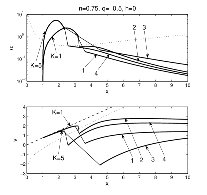
Figure 2: Global LH2 void solutions with shocks for parameters $(n=0.75,\ q=-0.5,\ \gamma=1.1875,\ h=0)$ and the void boundary $x^{*}=1$. The upper panel shows the reduced density $\alpha(x)$ and the lower panel shows the reduced radial velocity $v(x)$. In the upper panel, a logarithmic scale is used for $\alpha(x)$. In both panels, the dotted curve is the sonic critical curve, and in the lower panel the dashed curve is the void boundary line $nx-v=0$. The void solution with $K=1$ connects two solutions 1 and 2 whose parameters are: $A=7.3025,\ B=3.7802,\ x_{\rm sd}=3,\ \alpha_{\rm sd}=1.6366,\ v_{\rm sd}=1.9702,\ x_{\rm su}=3.6205,\ \alpha_{\rm su}=0.2519,\ v_{\rm su}=0.1559$ (solution 1), and $A=8.7808,\ B=6.3723,\ x_{\rm sd}=3.2,\ \alpha_{\rm sd}=1.1040,\ v_{\rm sd}=1.9755,\ x_{\rm su}=3.2529,\ \alpha_{\rm su}=0.3781,\ v_{\rm su}=1.1854$ (solution2), respectively. The void solution with $K=5$ connects two solutions 3 and 4 whose parameters are: $A=24.493,\ B=4.854,\ x_{\rm sd}=2.27,\ \alpha_{\rm sd}=2.8499,\ v_{\rm sd}=1.4515,\ x_{\rm su}=4.5410,\ \alpha_{\rm su}=0.2587,\ v_{\rm su}=-2.1237$ (solution 3), and $A=7.6878,\ B=5.4448,\ x_{\rm sd}=2.37,\ \alpha_{\rm sd}=2.0616,\ v_{\rm sd}=1.4308,\ x_{\rm su}=2.5603,\ \alpha_{\rm su}=0.3928,\ v_{\rm su}=-0.0456$ (solution4), respectively.

With $\alpha^{*}=0$ at the void boundary, the density first increases and then decreases as $x$ increases; and the radial velocity increases as $x$ increases. The density profiles of LH2 void solutions (see the upper panel of Figure 2) indicate a prominent shell-type morphology surrounding a central cavity in expansion. The peak density of the solution and the width of the shell is modulated primarily by $K$ parameter, which varies for different astrophysical gas flow systems. With different values of $x_{\rm sd}$, different dynamic behaviours of the corresponding upstream side can be obtained (e.g. the lower panel of Figure 2). In the vicinity of the upstream shock front, the fluid can be either an inflow (solutions 1 and 2) or an outflow (solutions 3 and 4). With adopted parameters, the fluid always merges into an asymoptotic outflow (parameter $B>0$) far from the system centre, whereas it possible to construct solutions with $B\leq 0$ for LH2 voids (see MHD examples below and examples in Figure 6 for a conventional polytropic gas). Numerical explorations indicate that it is generally not possible to make LH2 void solutions to cross the sonic critical curve smoothly. In other words, the inclusion of hydrodynamic shocks is necessary in order to construct sensible semi-complete global void solutions.

The possibility of asymptotic inflows at large $x$ associated with central void solutions deserves special attention. Without shocks, void solutions generally merge into asymptotic expansion solutions with flow velocities remaining positive. This establishes the physical links between central expanding voids and asymptotic outflows. In the presence of shocks, the upstream may have inflows, either near the shock front or sufficiently far from the system centre. This means that initially and at large radii a cloud system may involve inflow or contraction under the self-gravity. When the central engine forms an expanding void, a resulting shock may face the falling gas and expand outwards. For example, in Hu & Lou (2008a), the possibility of asymptotic inflows at large $x$ is interpreted as a special scenario for “champagne flows” in H II regions.

We emphasize that LH2 solutions here are the only void solutions in non-magnetized cases with $\alpha^{*}=0$. The shell-type appearance is a general feature for LH2 void solutions. Such solutions are applicable to shell-type morphologies, widely observed in various astrophysical gas systems, such as supernova remnants and hot bubbles (e.g. Ferrièrre 1998, 2001), H II regions (e.g. Hu & Lou 2008a) and even cavities in galaxy clusters (e.g. McNamara et al. 2005). The increasing velocity with radius of such solutions suggests a wind nature: the fast wind from the central cavity decelerates in the shell and the mass is accumulated in the shell. This is consistent with the picture of champagne flows of H II regions (e.g. Hu & Lou 2008a) and supernova remnants.

3.2 MHD Cases

With a random magnetic field, both LH1 and LH2 void solutions exist. As counterparts to hydrodynamic cases, we consider LH2 void solutions with the same parameters adopted in the previous section, except for the magnetic parameter being $h=0.3$. Such global MHD LH2 void solutions with shocks are shown in Figure 3.

Figure 3: Global MHD LH2 void shock solutions with parameters $(n=0.75,\ q=-0.5,\ \gamma=1.1875,\ h=0.3)$ and a void boundary $x^{*}=1$. The same format is adopted as in Figure 2. The void solution with $K=1$ does not allow a magnetosonic shock and it merges into the MHD free-expansion solution. The void solution of $K=5$ connects with solutions 1 and 2 whose parameters are: $A=12.325,\ B=3.977,\ x_{\rm sd}=4,\ \alpha_{\rm sd}=0.4915,\ v_{\rm sd}=2.2888,\ x_{\rm su}=5.5577,\ \alpha_{\rm su}=0.1273,\ v_{\rm su}=0.3533$ (solution 1), and $A=18.390,\ B=8.344,\ x_{\rm sd}=7,\ \alpha_{\rm sd}=0.2401,\ v_{\rm sd}=4.2102,\ x_{\rm su}=8.6661,\ \alpha_{\rm su}=0.0941,\ v_{\rm su}=3.2135$ (solution 2), respectively. The void solution of $K=10$ connects with solutions 3 and 4 whose parameters are: $A=7.5520,\ B=4.010,\ x_{\rm sd}=4,\ \alpha_{\rm sd}=0.4478,\ v_{\rm sd}=2.1273,\ x_{\rm su}=4.2913,\ \alpha_{\rm su}=0.1775,\ v_{\rm su}=0.8558$ (solution 3), and $A=15.175,\ B=7.706,\ x_{\rm sd}=7,\ \alpha_{\rm sd}=0.2317,\ v_{\rm sd}=4.1652,\ x_{\rm su}=8.0096,\ \alpha_{\rm su}=0.0999,\ v_{\rm su}=3.1276$ (solution 4), respectively.

The appearance of MHD LH2 void solution does not change very much with a magnetic parameter $h>0$. The density profiles also show shell-type morphology and the velocity still increases with radius (see Fig 3). Compared with non-magnetized cases shown in Figure 2 with the same void boundary $x^{*}$ and the same parameter $K$, the peak density in the shell is lower and the shell width appears broadened in MHD cases. The $K=1$ void solution in the non-magnetized case can involve a shock, otherwise it encounters the SCC. However, with the same value of $K$ in the magnetized case, the void solution cannot harbor any shocks and merge into the MHD free-expansion solution definitely. The $K=5$ and $K=10$ void solutions in the magnetized case can harbor MHD shocks. The MHD behaviour of the corresponding upstream sides, from our numerical exploration, is all outflow (Solutions 1, 2, 3 and 4 of Fig 3). With a larger $x_{\rm sd}$, or a faster shock, the upstream outflow has larger velocity, both near the shock front and far from the centre. The shell-type appearance is commonly observed for LH2 void solutions, for hydrodynamic and MHD cases.

We now consider MHD LH1 void solutions, for which the void boundary $nx-v=0,\ \alpha=0$ is also a critical curve and the asymptotic solution approaching the void boundary is an eigensolution. The regime of parameter in which the LH1 void solution exists is $q>0,\ \gamma+q\geq 1,\ h>0$ ($\gamma\geq 1$). Examples of MHD LH1 void solutions are shown in Fig 4, which do not encounter the critical curve and approach free-expansion asymptotic solution (37) at large $x$. For this reason, the three velocity curves in the bottom panel of Fig 4 are nearly identical. The density and velocity increases as $x$ increases. With a larger parameter $q$, the density profile appears more pronounced in the vicinity of void boundary. Because the free-expansion solution has infinite velocity and constant density far from the flow centre, the LH1 void solutions would be more suitable for astrophysical model if they are matched with another branch of solution with finite velocity and density at large $x$ by MHD shocks. Examples of shocks are shown in Fig 4 for $q=0.3$ with downstream shock positions $x_{\rm sd}=3$, $x_{\rm sd}=5$, and $x_{\rm sd}=8$, respectively. Again with a larger $x_{\rm sd}$, or a faster shock, the upstream outflow has a higher speed.

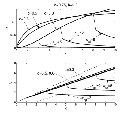
Figure 4: Semi-complete global MHD LH1 void solutions and shocks with the parameter $(n=0.75,\ h=0.3)$ and the void boundary $x^{*}=1$. The same format as Figure 2 is adopted. The void solutions merge to the free-expansion solution (37) and the constant value of $\alpha$ to be $\alpha_{\infty}=0.238$ (equation 40). The void solution of $q=0.3$ connects with three upstream solutions whose parameters are: $A=0.0968,\ B=1.6372,\ x_{\rm sd}=3,\ \alpha_{\rm sd}=0.0299,\ v_{\rm sd}=2.3340,\ x_{\rm su}=3.1374,\ \alpha_{\rm su}=0.0120,\ v_{\rm su}=1.8694$; $A=0.9024,\ B=2.8925,\ x_{\rm sd}=5,\ \alpha_{\rm sd}=0.0774,\ v_{\rm sd}=3.7655,\ x_{\rm su}=5.1942,\ \alpha_{\rm su}=0.0353,\ v_{\rm su}=3.0033$; and $A=5.0384,\ B=5.2269,\ x_{\rm sd}=8,\ \alpha_{\rm sd}=0.1300,\ v_{\rm sd}=5.8366,\ x_{\rm su}=8.2401,\ \alpha_{\rm su}=0.0689,\ v_{\rm su}=4.7681$, respectively.

Examples of MHD LH1 void solutions for the relativistic case of $q=2/3,\ \gamma=4/3$ are displayed in Fig. 5. We set free parameter $C=1$ and the arbitrary parameter $\lambda$ on the shock to be $\lambda=1$. With equations (12) and (13), we obtain the MCC with $\alpha=0.3897$ and $v=0.0151x$. In this case, the suitable expansion solution becomes the Einstein-de Sitter solution as shown in Fig. 5. Similarly, we are able to construct MHD shocks to match LH1 void solutions with another branch of solution (32) with finite velocity and density far from the flow centre.

In general, the reduced density of MHD LH1 void solutions increases with increasing $x$, and the density near the upstream side of shock is very low, as compared with the density near the downstream side of shock (see Figs. 4 and 5 for shocks). For the corresponding upstream solutions, the density decreases as $x$ increases and tends to zero at large $x$. With MHD shocks, we obtain again the shell-type morphology for the density. This shell-type morphology here is somehow different from the shell-type morphology of LH2 void solutions (e.g. Figs. 2 and 3). The LH2 void solutions have density peaks near the void boundary by themselves: the density increases and then decreases with increasing $x$. However, the LH1 void solutions must involve MHD shocks to have shell-type density profiles and the peak density is located on the downstream side of shock.

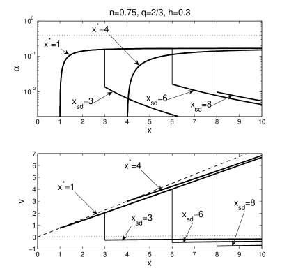
Figure 5: Semi-complete global MHD LH1 void shock solutions with parameters $n=0.75,\ q=2/3,\ \gamma=4/3,\ h=0.3,\ C=1$ and the void boundary $x^{*}=1$ and $x^{*}=4$. The same format as Figure 2 is adopted. The MCC is $\alpha=0.3897,\ v=0.0151x$. The inner void solution of $x^{*}=1$ connects with two upstream solutions whose parameters are: $A=0.2819,\ B=-0.3660,\ x_{\rm sd}=3,\ \alpha_{\rm sd}=0.1577,\ v_{\rm sd}=2.0388,\ x_{\rm su}=3,\ \alpha_{\rm su}=0.0136,\ v_{\rm su}=-0.2542$; and $A=2.0920,\ B=-0.7974,\ x_{\rm sd}=6,\ \alpha_{\rm sd}=0.1666,\ v_{\rm sd}=4.0166,\ x_{\rm su}=6,\ \alpha_{\rm su}=0.0163,\ v_{\rm su}=-0.4443$, respectively. The inner void solution of $x^{*}=4$ connects to one upstream solution whose parameters are: $A=2.7441,\ B=-1.5525,\ x_{\rm sd}=8,\ \alpha_{\rm sd}=0.1404,\ v_{\rm sd}=5.5306,\ x_{\rm su}=8,\ \alpha_{\rm su}=0.0097,\ v_{\rm su}=-0.7679$.

4 Hydrodynamic Self-Similar Void Solutions with $\alpha^{*}\neq 0$

By setting magnetic parameter $h=0$, we readily obtain a group of self-similar nonlinear ODEs describing the hydrodynamics of a general polytropic gas with specific entropy conserved along streamlines. We shall choose a non-zero $\alpha^{*}$ at the void boundary $nx-v=0$, or parameter $K$, in constructing solutions with a considerable freedom. We also insert hydrodynamic shocks to obtain semi-complete global solutions satisfying the asymptotic condition that $v(x\rightarrow\infty)=0$. According to Table 1, asymptotic behaviours near the void boundary can be generally classified as Type-N ($q=0,\ n\neq 1$), Type-N2 ($q=0,\ n=1$) and Type-D ($q>0$) separately.

4.1 Cases of $q=0$

With $q=0$ and $h=0$, the flow system is reduced to a conventional polytropic gas obeying $n+\gamma=2$ and have a constant specific entropy everywhere at all times. Such hydrodynamic flows are systematically and carefully analyzed and discussed by Wang & Lou (2007). Hu & Lou (2008a) constructed void solutions in a conventional polytropic flow to model the so-called ‘champagne flows’ in H II regions. In Figure 6, we present examples of void solutions with hydrodynamic shocks across the sonic singular surface. For the same void solution, by properly choosing the downstream shock position $x_{\rm sd}$, we can obtain various dynamic behaviours on the upstream side: outflow (e.g. $B>0$ in solution 3 of Figure 6), inflow (e.g. $B<0$ in solution 1 of Figure 6) and contraction (e.g. $B=0$ in solution 2 of Figure 6). Basically, upstream dynamic behaviours depend on the void boundary $x^{*}$, the density at the void boundary $\alpha^{*}$, and the downstream shock position $x_{sd}$. Extensive numerical explorations reveal that the isothermal case (Type-N2) is similar to other $q=0$ cases regarding the void solutions. Lou & Zhai (2009) provide a detailed analysis for isothermal voids.

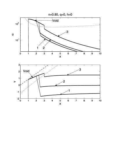
Figure 6: Void solutions with $n=0.85$, $\gamma=1.15$, $q=0$, $h=0$ for a conventional polytropic gas. The same format as Fig. 2 is adopted. The void solution of $x^{*}=1,\ \alpha^{*}=2$ connects with solutions 1, 2 and 3 whose parameters are: $A=2.2257,\ B=-1.8402,\ x_{\rm sd}=2,\ \alpha_{\rm sd}=1.4849,\ v_{\rm sd}=1.3202,\ x_{\rm su}=2.5521,\ \alpha_{\rm su}=0.1870,\ v_{\rm su}=-1.6783$ (solution 1); $A=2.5682,\ B=0,\ x_{\rm sd}=2.314,\ \alpha_{\rm sd}=1.2452,\ v_{\rm sd}=1.4646,\ x_{\rm su}=2.4721,\ \alpha_{\rm su}=0.2797,\ v_{\rm su}=-0.2876$ (solution 2); and $A=6.4646,\ B=3.2026,\ x_{\rm sd}=3,\ \alpha_{\rm sd}=0.8228,\ v_{\rm sd}=1.7353,\ x_{\rm su}=3.0056,\ \alpha_{\rm su}=0.5033,\ v_{\rm su}=1.2203$ (solution 3), respectively.

4.2 Cases of $q>0$

For $q>0$, asymptotic solution behaviours at the void boundary are of Type-D. We can construct void solutions with shocks. Examples of such void shock solutions with different values of $q$ are shown in Figs 7 and 8.

Dynamic behaviours of void solutions depend on the void boundary $x^{*}$ and the density parameter $K$. Without encountering the sonic critical point, some void solutions (see curves $2$, $3$ and $4$ in Fig 7) merge into one kind of asymptotic expansion solutions (e.g. asymptotic free-expansion solution, with $v\sim 2x/3$ for $q<2/3$, Einstein-de Sitter solution for $q=2/3$, or asymptotic thermal-expansion solution for $q>2/3$). As shown by Figure 7, void solutions with different void boundaries merge into the same asymptotic free-expansion solution, except for a slightly different $b$ parameter. Again, we shall connect these solutions with another asymptotic solution of finite velocity and density at large $x$ by shocks (see curves $5$ and $6$ in Fig. 7). By properly choosing the downstream shock position, we could readily obtain an inflow ($v<0$) or an outflow ($v>0$) for the upstream side of a shock. The radial flow velocity tends to zero at large radii. Some void solutions cross the critical curve smoothly (see curve 1 in Fig. 7).

Figure 7: Inflow velocities $-v(x)$ of void solutions with $n=0.85$, $\gamma=1.2875$, $q=0.5$, $h=0$. The upper dotted curve is the sonic critical curve (SCC), and the lower dotted curve is the void boundary $nx-v=0$. The solid curve 1 is a void solution with $x^{*}=0.4$, crossing the upper SCC smoothly at $x=4$, and matching asymptotic solution (32) with $A=19.852$ and $B=1.286$. Solid curves 2, 3, 4 are integrated from $x^{*}=1$, $x^{*}=2$, $x^{*}=3$, with $K=0.29$, and $v^{\prime}$ given by expression (16). These solutions merge to the free expansion asymptotic solutions with form $v=2x/3+b,\ \alpha_{\infty}=2/3$. The void solution of $x^{*}=1$ and $K=0.29$ connects with solutions 5 and 6 whose parameters are: $A=3.241,\ B=-0.987,\ x_{\rm sd}=2,\ \alpha_{\rm sd}=0.502,\ v_{\rm sd}=1.246,\ x_{\rm su}=4.045,\ \alpha_{\rm su}=0.114,\ v_{\rm su}=-0.607$ (solution 5), and $A=2.173,\ B=-0.143,\ x_{\rm sd}=2.4,\ \alpha_{\rm sd}=0.435,\ v_{\rm sd}=1.479,\ x_{\rm su}=3.425,\ \alpha_{\rm su}=0.126,\ v_{\rm su}=0.136$ (solution 6), respectively.

As shown in Fig. 8 of a relativistically hot gas, the critical curve can be obtained analytically from equations (12) and (13) with $\alpha=3.2843$ and $v=-2.1772x$. Void solutions merge into the Einstein-de Sitter solution as expected. The Einstein-de Sitter solution has a diverging velocity at large $x$. Again, this solution can be connected with an asymptotic solution (32) of finite velocity and density at large $x$ via shocks.

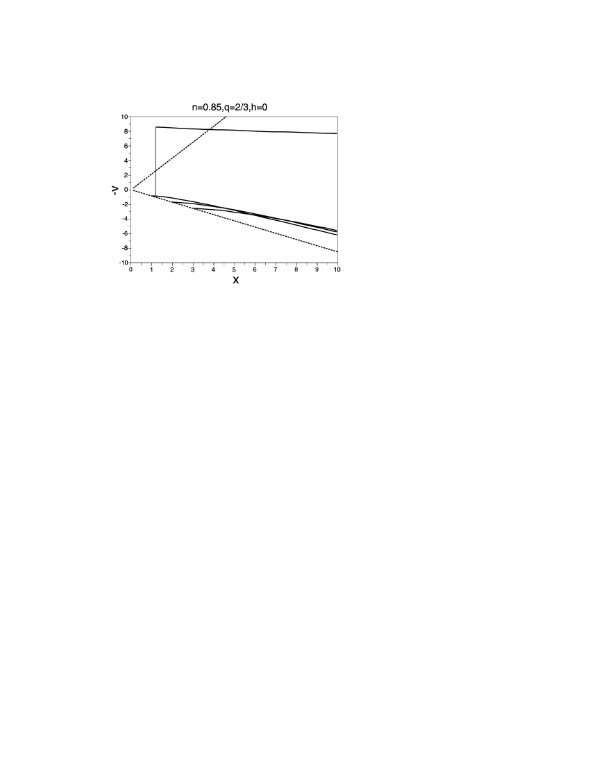
Figure 8: Void solutions and the Einstein-de Sitter solution with $n=0.85$, $\gamma=4/3$, $q=2/3$, $h=0$ and $C=1$. Inflow velocities $-v(x)$ are presented. The same format as Figure 7 is adopted. The critical curve is $v=-2.1772x$. The solid curves are integrated from the void boundary at $x^{*}=1$, $x^{*}=2$, $x^{*}=3$, with $K=0.2$ and $v^{\prime}$ given by expression (16), which match with the Einstein-de Sitter solution at large $x$. The void solution with $x^{*}=1,\ K=0.2$ connects to one upstream solution whose parameters are: $A=0.188,\ B=-12.131,\ x_{\rm sd}=1.2,\ \alpha_{\rm sd}=3.453,\ v_{\rm sd}=0.874,\ x_{\rm su}=1.2,\ \alpha_{\rm su}=0.0524,\ v_{\rm su}=-8.566$.

5 MHD Self-Similar Void Solutions with $\alpha^{*}\neq 0$

The magnetic force may play a key role in the vicinity of void boundary and smooths out all divergence of the non-magnetized cases. In a MHD flow ($q\geq 0$), $\alpha^{*}=0$ at the void boundary is allowed for non-trivial void solutions with $h>0$, e.g. MHD LH1 void solution. In this section, we compare $\alpha^{*}=0$ and $\alpha^{*}>0$ cases, and see if the boundary value of $\alpha^{*}$ modifies characteristic behaviours of void solutions.

5.1 Case of  $q=0$ for a conventional polytropic gas

Examples of global MHD void solutions for the case of $q=0$ are shown in Fig. 9. Numerical computations show that along the MCC, velocity gradient $v^{\prime}$ has one positive and another negative eigenvalues, corresponding to the MCC being saddle points (e.g. Jordan & Smith 1977). Solutions approaching this MCC, may either cross the critical curve smoothly and match with asymptotic solution (32) of finite velocity and density at large $x$ (see solution curve 1 in Fig. 9), or be turned back smoothly to match with another branch of solutions and merge into the Einstein-de Sitter solution at large $x$ (see solution curves 2, 3 and 4 in Fig. 9). By adjusting the $\alpha^{*}$ value at the void boundary, we can make the solution crossing the MCC smoothly. The only difference to integrate curves 1 and 2 in Fig. 9 is the $\alpha^{*}$ value. Compared with the case without magnetic field (see Fig. 6), a void solution in this case can merge into the Einstein-de Sitter solution at large $x$ without encountering the MCC. Void solutions can be connected with outer branch of the asymptotic solutions of finite velocity and density by MHD shocks (see solution curves 5 and 6 in Fig. 9). Similarly by adjusting the downstream shock position $x_{sd}$, one void solution on the downstream side can be connected to various upstream solutions with different behaviours at large $x$.

Figure 9: MHD void solutions with $n=0.85$, $\gamma=1.15$, $q=0$ and $h=0.3$. Inflow velocities $-v$ are plotted. The same format as Fig. 7 is adopted. Solid curve 1 is a void solution with $x^{*}=1$ and $\alpha^{*}=5$, crossing the MCC smoothly at $x=4$ to match with asymptotic solution (32) with $A=32$ and $B=5.413$ at large $x$. Solid curves 2, 3, 4 are integrated from the void boundary at $x^{*}=1$, $x^{*}=2$, $x^{*}=3$ respectively all with $\alpha^{*}=2$ and $v^{\prime}$ given by expression (25). These solutions are limited by the upper MCC and merge into the Einstein-de Sitter solutions $(v=2x/3\ ,\ \alpha=\hbox{ const})$. The void solution of $x^{*}=1$ and $\alpha^{*}=2$ connects with solutions 5 and 6 whose parameters are: $A=0.205,\ B=4.280,\ x_{\rm sd}=3,\ \alpha_{\rm sd}=0.556,\ v_{\rm sd}=1.714,\ x_{\rm su}=3.159,\ \alpha_{\rm su}=0.191,\ v_{\rm su}=0.123$ (solution 5), and $A=0.169,\ B=1.128,\ x_{\rm sd}=2.2,\ \alpha_{\rm sd}=0.868,\ v_{\rm sd}=1.356,\ x_{\rm su}=3.306,\ \alpha_{\rm su}=0.126,\ v_{\rm su}=-2.492$ (solution 6), respectively.

5.2 Case of  $q>0$

An example of $q=0.5$ is shown in Fig. 10, which can be compared with Fig. 7. The case of $q=2/3$ describes a relativistically hot gas. MHD void solutions in such case is shown in Fig. 11 for a comparison with Fig. 8.

Again the density at the void boundary $\alpha^{*}$ can be set to either zero, which leads to the LH1 void solution with eigensolution (15) (see curves $2,\ 3$ and $4$ of Fig. 10, and curve 1 of Fig. 11), or a nonzero finite value, which leads to a Type-Nq behaviour of equations (27)$-$(2.2.3) (see curves $2^{\prime},\ 3^{\prime}$ and $4^{\prime}$ of Fig. 10, and curves $2$ and $2^{\prime}$ of Fig. 11). In the absence of a magnetic force, only the Type-D behaviour is allowed in this range of $q$ and the density diverges on the void boundary. If not encountering the MCC, these solutions merge into one kind of expansion solutions at large $x$ (i.e. free-expansion for $q<2/3$, Einstein-de Sitter solution for $q=2/3$, and thermal-expansion for $q>2/3$). This property is the same as hydrodynamic cases, and we note that the constant density $\alpha_{\infty}$ of the free-expansion solution does depend on the magnetic parameter $h$. This suggests that for such void solutions, the magnetic force plays an important role. Similar to non-magnetized cases, we can avoid the velocity divergence of the expansion solutions by matching such solutions with asymptotic solutions of finite velocity and density at large $x$ via MHD shocks (e.g. curves $5,\ 6$ and $7$ of Fig. 10, and curves 3, 4 and 5 of Fig. 11), or making the void solutions crossing the MCC smoothly (see curve 1 of Fig. 10 and compare it with curve 1 of Fig. 7). From Figs. 10 and 11, the LH1 void solutions and the Type-Nq behaviour appear quite similar in terms of velocity profiles, except near the void boundary and different $b$ parameter in the corresponding expansion solutions. We will discuss the influence of the initial mass density $\alpha^{*}$ presently.

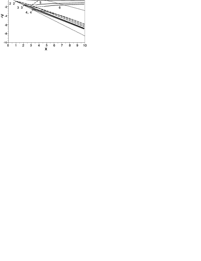
Figure 10: MHD void solutions with $n=0.85$, $\gamma=1.2875$, $q=0.5$, $h=0.3$. Inflow velocities $-v(x)$ are plotted. The same format as Fig. 7 is adopted. The solid curve 1 is a void solution with the void boundary at $x^{*}=0.3$, crossing the MCC smoothly at $x=5$ to match with asymptotic solution (32) with $A=25.977$ and $B=1.147$. The solid curves 2, 3, 4 are MHD LH1 void solutions, numerically integrated from the void boundary at $x^{*}=1$, $x^{*}=2$, $x^{*}=3$ with $\alpha^{*}=0$. Respectively, the dashed curves $2^{\prime}$, $3^{\prime}$, $4^{\prime}$ are Type-Nq void solutions, integrated from the void boundary at $x^{*}=1$, $x^{*}=2$, $x^{*}=3$ with $\alpha^{*}=2$. These solutions merge into the free expansion asymptotic solutions in the form of $v=2x/3+b$ at large $x$ with $\alpha_{\infty}=0.238$. The void solution 2 of $x^{*}=1,\alpha^{*}=0$ connects with solutions 5 and 6 whose parameters are: $A=0.256,\ B=1.692,\ x_{\rm sd}=2,\ \alpha_{\rm sd}=0.0646,\ v_{\rm sd}=1.475,\ x_{\rm su}=3.662,\ \alpha_{\rm su}=0.0182,\ v_{\rm su}=1.648$ (solution 5), and $A=0.805,\ B=2.119,\ x_{\rm sd}=3,\ \alpha_{\rm sd}=0.0943,\ v_{\rm sd}=2.142,\ x_{\rm su}=4.731,\ \alpha_{\rm su}=0.0299,\ v_{\rm su}=1.991$ (solution 6), respectively. The void solution 2’ of $x^{*}=1$ and $\alpha^{*}=2$ connects with solution 7 whose parameters are: $A=2.610,\ B=0.208,\ x_{\rm sd}=3,\ \alpha_{\rm sd}=0.292,\ v_{\rm sd}=1.772,\ x_{\rm su}=4.142,\ \alpha_{\rm su}=0.102,\ v_{\rm su}=0.445$.

The MCC has the form $\alpha=3.0088,\ v=-2.2087x$ for the case of $C=1$, $\gamma=4/3$, $n=0.85$, $q=2/3$ and $h=0.3$. The behaviour of MHD void solutions is similar to the hydrodynamic case. In such cases, it is unlikely for void solutions to encounter the MCC and the only way they cross this singular surface is via MHD shocks (see curves $3,\ 4$ and $5$ in Fig. 11).

Figure 11: MHD void solutions with $n=0.85$, $\gamma=4/3$, $q=2/3$, $h=0.3$ and $C=1$. $-v$ is plotted. The upper dotted curve is the MCC satisfying $v=-2.2087x$ and the lower dotted curve is the void boundary $nx-v=0$. The solid curves 1 is LH1 void solution, integrated from the void boundary at $x^{*}=1$ with $\alpha=0$. The solid curves $2$ and $2^{\prime}$ are Type-Nq void solutions, integrated from the void boundary at $x^{*}=1$ with $\alpha^{*}=2$ and $\alpha^{*}=10$. These solutions merge into the Einstein-de Sitter solution at large radii. The void solution 1 of $x^{*}=1,\alpha^{*}=0$ connects with solutions 3 and 4 whose parameters are: $A=0.379,\ B=1.255,\ x_{\rm sd}=3,\ \alpha_{\rm sd}=0.114,\ v_{\rm sd}=2.095,\ x_{\rm su}=3,\ \alpha_{\rm su}=0.0413,\ v_{\rm su}=1.292$ (solution 3); and $A=0.848,\ B=1.680,\ x_{\rm sd}=4,\ \alpha_{\rm sd}=0.123,\ v_{\rm sd}=2.750,\ x_{\rm su}=4,\ \alpha_{\rm su}=0.0459,\ v_{\rm su}=1.661$ (solution 4), respectively. The void solution 2’ of $x^{*}=1$ and $\alpha^{*}=10$ connects with solutions 5 whose parameters are: $A=2.699,\ B=-4.921,\ x_{\rm sd}=3,\ \alpha_{\rm sd}=0.864,\ v_{\rm sd}=1.544,\ x_{\rm su}=3,\ \alpha_{\rm su}=0.149,\ v_{\rm su}=-3.298$.

We further investigate the influence of $\alpha^{*}$ value at the void boundary on semi-complete global solutions. By comparing solutions from the same void boundary $x^{*}$ and different $\alpha^{*}$ values (see curves $1,\ 2,\ 2^{\prime}$ in Fig. 11), it appears that with larger $\alpha^{*}$ on the void boundary, the void solutions converge to the asymptotic solution more slowly. This means that with larger density gradient on the void boundary, the system has a larger transition zone where the magnetic force, the gravity and the thermal pressure force are all comparable. We refer to this zone as the void boundary layer. Outside the void boundary layer, the free expansion, thermal expansion or the Einstein-de Sitter solution would be a good approximation for the asymptotic behaviour. With an MHD shock inserted, the solution can be matched with an outflow (curves 3 and 4 in Fig. 11) or an inflow (curve 5 in Fig. 11). The dynamic behaviour of the outer upstream flow of the global void solution depends on the void boundary $x^{*}$, the value of $\alpha^{*}$ and the downstream shock point $x_{\rm sd}$. From the same void boundary $x^{*}$, we can adjust $\alpha^{*}$ values to let the solution either cross the MCC smoothly or merge into asymptotic expansion solutions (see curves 1 and 2 in Fig. 9).

As a further discussion, we obtain void solutions with different $\alpha^{*}$ values at the void boundary with parameters $(n=0.85,\ \gamma=1.7,\ q=2,\ h=0.3)$ (see Figure 12). In such cases, there is no MCC. The solution curves are very similar and merge quickly as a single curve (i.e. asymptotic thermal expansion solution). This suggests that the general behaviour of the void solution is not influenced by the initial $\alpha^{*}$ value. In other words, $\alpha^{*}$ at the void boundary is fairly arbitrary and only influences the dynamical behaviour near the void boundary (e.g. void boundary layer). For a realistic astrophysical flow, the dynamics on the void boundary cannot be described in a self-similar manner, due to unavoidable diffusion processes. Therefore, choices of $\alpha^{*}$ at the void boundary in our model serve only for starting a numerical integration. A more complete understanding of such system requires information for the relations between the $\alpha^{*}$ value on the void boundary and the initial physical conditions that generate voids, such as density perturbations and growths in supernova explosions (e.g. Cao & Lou 2009) or hot fast winds in planetary nebulae (e.g. Lou & Zhai 2009).

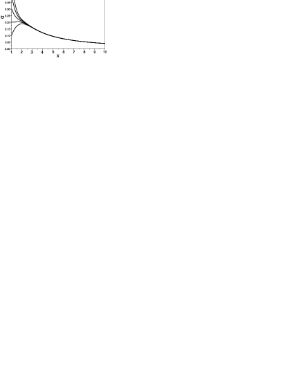
Figure 12: Influence of the initial value of $\alpha^{*}$ on the void solution. The five flow solution curves are integrated with $n=0.85$, $\gamma=1.7$, $q=2$, $h=0.3$, from the void boundary at $x^{*}=1$, and different initial values of $\alpha^{*}=0.5,\ 0.4,\ 0.3,\ 0.2,\ 0.1$ are chosen. The $v(x)$ part of these five solutions are nearly identical (not shown here). From this figure, for $x>2.5$, the five curves merge together, therefore the influence of the initial value of $\alpha^{*}$ is only significant around $1<x<2.5$.

6 Astrophysical Applications

Our self-similar solutions can be adapted to different astrophysical flow systems with various spatial and temporal scales. The sound parameter $k$ determines the dimensional quantities in physical space and $k$ varies for different astrophysical flow systems. From self-similar transformation (6), we have a relation

$$k^{1-3q/2}=\frac{p}{(4\pi G)^{\gamma-1}G^{q}(3n-2)^{q}\rho^{\gamma}M^{q}}$$

$$=\frac{k_{B}T}{\mu(4\pi G)^{\gamma-1}G^{q}(3n-2)^{q}\rho^{\gamma-1}M^{q}}\ \ ,$$ (43)

where $T$ is the thermal temperature, $k_{B}$ is Boltzmann’s constant, $\mu$ is the mean molecular (atomic) mass of gas particles and the second equality only holds for an ideal gas. Since the entropy is closely related to $p\rho^{-\gamma}$, the increase of entropy across a shock front from the upstream side to the downstream side would lead an increase of $k$ value in the same direction for $q<2/3$. For $\gamma>1$ and $q<2/3$, the temperature should also increase across a shock front in the same direction. It is still not trivial to estimate $k$ values from relation (43) above, because the enclosed mass $M$ varies in $r$. Numerical tests show that when $q$ is not too large, setting $q=0$ does not influence the magnitude order of $k$ value. Thus we use a simplified relation

$$k=\frac{p}{\rho^{\gamma}(4\pi G)^{\gamma-1}}=\frac{k_{B}T}{\mu\rho^{\gamma-1}(4\pi G)^{\gamma-1}}\ .$$ (44)

This is identical with relation (59) of Lou & Wang (2006) for a conventional polytropic gas. The relation does depend on the value of $\gamma$. For a late evolution phase of massive stars after the hydrogen burning, the central density and temperature are $\rho_{c}\sim 10^{8}$ g cm^-3 and $T_{c}\sim 10^{9}$ K. We estimate $k\sim 10^{16}-10^{17}$ cgs unit, depending on the value of $\gamma$. For the interstellar medium (ISM) in our own Galaxy, mainly composed of hydrogen, $\rho_{\rm ISM}\sim 10^{-20}-10^{-26}$ g cm^-3 and $T_{\rm ISM}\sim 10-10^{6}$ K (e.g. Ferrière et al. 2001) and we estimate $k\sim 10^{9}-10^{24}$ cgs unit, depending on the value of $\gamma$ in the range of $1\;\lower 4.0pt\hbox{${\buildrel\displaystyle<\over{\sim}}$}\;\gamma\;\lower 4.0pt\hbox{${\buildrel\displaystyle<\over{\sim}}$}\;4/3$.

The parameters we have adopted in our model are $(n,\ \gamma,\ q,\ h)$ with the relation $\gamma=2-n+(3n-2)q/2$. The physical meaning of these parameters is clear. Parameters $(n,\ \gamma,\ q)$ are relevant for general polytropic processes. By setting $q=0$, we retrieve the conventional polytropic gas with a constant specific entropy everywhere at all times and require $n+\gamma=2$. The polytropic index $\gamma$ is an approximation commonly invoked when energetic processes are not known (e.g. Weber & Davis 1967). For example, when applying our model to an exploding stellar envelope, such as supernovae, $\gamma$ would be close to unity, indicating a tremendous energy deposit. To apply our model to a slowly-evolving ISM, $\gamma$ should be very close to ratio of specific heats $c_{\rm p}/c_{\rm v}$ for an adiabatic process. This is consistent with the dynamic evolution shown by our self-similar solutions. For a fixed $x$ value, the corresponding radius $r$ expands with time obeying a power law of $\sim t^{n}$. For $n>1$, $r$ expands faster and faster, implying a continuous energy input into a gas flow. Another role of $n$ is that it scales the initial density distribution of a gas flow. According to asymptotic solution (32), the mass density scales as $x^{-2/n}$ at large $x$. The initial condition with $t\rightarrow 0^{+}$ corresponds to the asymptotic boundary condition with $x\rightarrow\infty$, so the scaling parameter $n$ determines the initial density profile when the solution takes asymptotic form (32) at large $x$.

Our general shock void solutions may be adapted to model planetary nebulae. In the late stages of stellar evolution, the compact star becomes an intense source of hot fast stellar wind and photoionization. The fast wind catches up with the fully photoionized slow wind and supports a fast wind bubble of hot gas. Chevalier (1997) developed an isothermal self-similar model without self-gravity to study the expansion of a photoionized stellar wind around a planetary nebula (see also Meyer 1997). The key idea of Chevalier (1997) is that the inner edge of the slow wind forms a contact discontinuity with the stationary driving fast wind. We have shown that this contact discontinuity in gravity-free cases corresponds to the void boundary in our formulation. Lou & Zhai (2009) presented an isothermal model planetary nebula involving an inner fast wind with a reverse shock; this shocked wind is connected to an expanding self-similar void solution through an outgoing contact discontinuity. In their model, the self-gravity is included and a variety of flow profiles are possible. We here provide a theoretical model formulation in a more general framework with a polytropic equation of state and the inclusion of self-gravity and the magnetic force. Our MHD shocked void solutions are also suitable to describe the self-similar dynamics of planetary nebulae combined with effects of central stellar winds and photoionization.

Another astrophysical context to apply our MHD void shock solutions is the expansion of H II regions surrounding new-born protostars, especially for “champagne flows” (e.g. Hu & Lou 2008a). Ultraviolet photons from nascent nuclear-burning protostars fully ionize and heat the surrounding gas medium and drive H II regions out of equilibrium. Such H II regions expand and gradually evolve to a “champagne flow” phase with outgoing shocks.

As a more detailed application of our void solutions, we revisit below the scenario for core-collapse supernovae, which has been investigated numerically over years (e.g. see Liebendörfer et al. 2005 for an overview). Neutrino-driven models are widely adopted for explaining the physical mechanism of type-II supernovae. The core collapse and bounce create a tremendous neutrino flux and within several hundred milliseconds after the core bounce, neutrino sphere is largely trapped and deposit energy and momentum in the dense baryonic matter. A typical scenario is that the neutrinos drive the stellar materials outwards, deposit large amount of outward momentum and re-generate the delayed rebound shock to push outwards. Janka & Müller (1995, 1996) successfully obtained numerical simulation for the first second of type-II supernovae based on such a scenario. Many recent numerical studies, with more careful consideration of the convection in the stellar envelope and diffusion processes, also confirm and consolidate the viability of such a neutrino reheating process (e.g. Buras et al. 2006; Janka et al. 2007, 2008). From simulations of Janka & Müller (1995, 1996) on progenitor stars with a mass range of $\sim 8-15M_{\odot}$, the neutrino sphere stops depositing energy $\sim 0.5$ s after the core bounce and then decouples from the baryonic matter. Once decoupled, neutrinos quickly escape from the stellar interior and may leave a cavity between the centre and the envelope within the exploding progenitor star. At the centre of the cavity may lay a nascent neutron star, a stellar mass black hole, or even shredded debris (e.g. Cao & Lou 2009).

We now show that the gravity of a remnant central object (if not completely destroyed by the rebound process) on the expanding stellar envelope may be neglected under certain situations. The equivalent Bondi-Parker radius $r_{\rm BP}$ is

$$r_{\rm BP}=\frac{GM_{*}}{2a^{2}}\ ,$$ (45)

where $M_{*}$ is the mass of the central object and $a$ is the sound speed of the surrounding medium, which mainly depends on temperature. Far beyond $r_{\rm BP}$, the gravity of a central mass may be ignored. In the following, we will see that at $\sim 1$ s after the core bounce, the stellar envelope has a temperature of the order of $\sim 10^{8}$ K (see Fig. 14) and a corresponding sound speed squared $a^{2}\sim 10^{17}\hbox{ cm}^{2}\hbox{ s}^{-2}$. With $M_{*}\sim M_{\odot}$, the Bondi-Parker radius at 1 s is estimated to be of the order of $\sim 10^{8}$ cm which is roughly the same as the void boundary. Therefore at the beginning, the gravity of the central object is only marginally ignorable. From self-similar transformation (6), the Bondi-Parker radius, which is proportional to $1/a^{2}\propto\rho/p$, has the time dependence of $t^{2-2n}$. The void boundary expands as $t^{n}$. As long as we require $n>2/3$, the Bondi-Parker radius expands slower than the void boundary; in other words, the gravity of the central object may be ignored shortly after the core bounce. We can then presume that the central cavity is an approximate void and apply our self-similar void solutions. Similar approximation has been applied to other astrophysical flow systems, in which the gravity of central object can be neglected with respect to the dynamics of the surrounding gas (e.g. see Tsai & Hsu 1995; Shu et al. 2002; Bian & Lou 2005 and Hu & Lou 2008 for applications to shocked “champagne flows” in H_II regions).

The model framework of self-similar dynamics described in this paper implies that the radius of a spherical shock $r_{s}$ evolves with time $t$ in a power-law manner, i.e. $r_{s}=k^{1/2}x_{s}t^{n}$. We may regard $k^{1/2}x_{s}$ and $n$ as two free parameters and attempt to fit the self-similar evolution to the results of a numerical simulation by Janka & Müller (1996; e.g. their case O3c with relevant parameters specified in the caption of our Figure 13). We use $k=4\times 10^{16}$ cgs unit for the inner part of the void solution (i.e. the downstream side of an outgoing shock). The best fit model is achieved at $n=1.57$ and the downstream shock position (or speed) of $x_{s}=7.36$ (see Fig. 13). The self-similar evolution fits almost perfectly with the simulation. It is striking to obtain such a good agreement for shock evolution, because the numerical simulation of Janka & Müller (1996) employed an equation of state that contains contributions from neutrinos, free nucleons, $\alpha$-particles and a representative heavy nucleus in nuclear statistical equilibrium. In other words, their model carries distinct features. With our simple approximation, we essentially parameterized all these complicated energetic processes by a general polytropic equation of state. We expect to obtain different best-fit scaling parameter $n$, in comparison with numerical results under different conditions, such as higher or lower initial neutrino luminosity. This fitting is suggestive that the polytropic approach is a fairly good approximation for shock evolution, and physically the rebound shock expands in a self-similar manner.

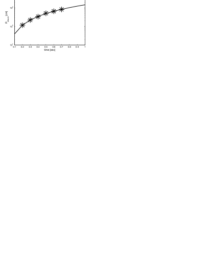
Figure 13: Shock positions as function of time after a core bounce. The solid curve shows the self-similar evolution, with parameters $n=1.57,\ k=4\times 10^{16}$ cgs unit and the downstream shock position $x_{s}=7.36$. The asterisks show the result of numerical simulation by Janka & Müller (1996) for a one-dimensional model of the core collapse of a progenitor with mass 15 M_⊙ and the iron core mass 1.31 M_⊙, and the initial neutrino luminosity 2.225$\times 10^{52}$ erg s^-1.

The numerical simulation of Janka & Müller (1996) ends at $\sim$ 1 s. Within this duration, neutrinos deposit enough momentum and kinetic energy in a shocked stellar envelope and the star is set to explode as the rebound shock emerges from the stellar photosphere. The subsequent dynamic evolution, including the travel of the rebound shock, can be readily described by our self-similar model. Soon after neutrinos decouple from the baryon matter, no more energy is provided and indeed the system begins to lose energy by radiation processes. Thus, we can no longer apply $n=1.57$ further. We therefore use their model parameters at $\sim 1$ s as the initial input parameters of subsequent dynamic evolution. We found that if $n=0.8,\ \gamma=1.2,\ q=0$ (i.e. a conventional polytropic gas), our self-similar model gives appropriate solutions and we do not include a random magnetic field in this preliminary illustration. The void solutions with these parameter are of Type-N and relevant examples are also shown in Fig. 6. The cavity radius is taken to be $\sim 1000$ km at $t=1$ s and the corresponding void boundary is then $x^{*}=0.5$. From the simulation case O3c of Janka & Müller (1996), the rebound shock is at $\sim 1.3\times 10^{9}$ cm at $t=1$ s, which correspond to a downstream shock position $x_{sd}=6.5$. We note that for these parameters the mass density cannot be set to zero at the void boundary, hence we should choose $\alpha^{*}$ properly such that the mass density on the void boundary at $t=1$ s is equal to the mass density given by the case 03c. The void solution at $t=1$ s is shown in Fig. 14.

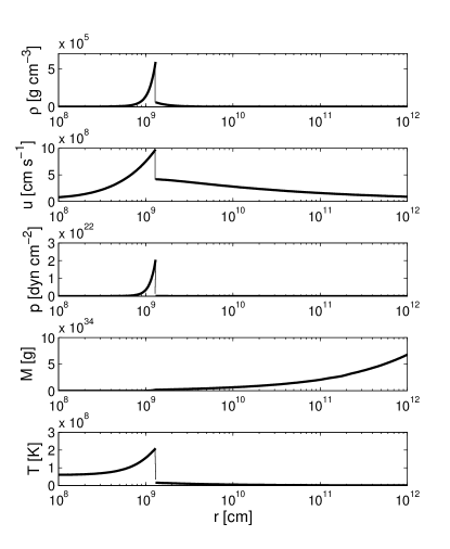
Figure 14: Self-similar void solution for an exploding progenitor star at $t=1$s. From top to bottom, the panels show the density, radial flow velocity, thermal pressure, enclosed mass and the thermal temperature. The solution is obtained with parameters $n=0.8,\ \gamma=1.2,\ q=0,\ h=0,\ k=4\times 10^{16}$ cgs unit, void boundary $x^{*}=0.5$, density at the void boundary $\alpha^{*}=0.001$ and the downstream shock position $x_{sd}=6.5$. Correspondingly at the moment shown, the void boundary is at $10^{8}$ cm and the rebound shock is at $1.3\times 10^{9}$ cm. Our solution is numerically integrated until $10^{12}$ cm.

The solution shown in Figure 14 corresponds well to the envelope of an exploding massive star. The enclosed mass is $\sim 25M_{\odot}$ with a radius of $\sim 10^{12}$ cm, grossly consistent with typical masses and radii of O and B stars. The enclosed mass mainly depends on the density $\alpha^{*}$ on the void boundary; by regarding $\alpha^{*}$ as a free parameter, the self-similar dynamics is capable of modelling stars with different masses. The solution shows an expansion velocity $\sim 10^{9}$ cm s^-1, a typical expansion velocity for type-II supernovae. The temperature increases from the void boundary to the rebound shock and decreases with $r$ outside the rebound shock. The temperature rises to $\sim 10^{8}$ K, grossly consistent with typical supernova temperature. Furthermore, we can compute the total energy of the entire system. We should consider the kinetic energy $E_{k}$, gravitational energy $E_{g}$ and the internal energy $E_{i}$. When calculating the internal energy, we assume that the gas is single-atomic, whose degree of freedom is 3. At $t=1$ s, the total energy $E_{total}$ is $6.54\times 10^{50}$ erg, in which the kinetic energy $E_{k}=1.63\times 10^{51}$ erg, the gravitational energy $E_{g}=-1.10\times 10^{51}$ erg, and the internal energy $E_{i}=1.21\times 10^{50}$ erg. We see that the kinetic energy is the major energy source, and the radial motion of the fluid has not been dissipated much to random motions, in agreement with the exploding star scenario. The total energy of our self-similar model is well consistent with the total energy $9.5\times 10^{50}$ erg given by the Case O3c of simulation (Janka & Müller 1996) which suggests that the energy of the stellar envelope of the self-similar model comes from the neutrino process before 1 s. Our calculations reveal that the energy does not vary much with time, consistent with our assumption that the system is nearly adiabatic. We conclude that in general, our self-similar void solution is plausible as it shows typical value of velocity, pressure, temperature, enclosed mass and total energy. We can also adjust the self-similar parameters to produce solutions for different objects.

Here we discuss two immediate utilizations of our self-similar solutions. First, as long as we know the evolution of a rebound shock, we can estimate the time when the shock breaks out of the stellar envelope. Assuming the stellar photosphere at a radius of $\sim 10^{12}$ cm, with the relation $r_{\rm shock}\propto t^{n}$, we estimate that the shock travels to the photosphere at $\sim 4\times 10^{3}$ s (i.e. $\;\lower 4.0pt\hbox{${\buildrel\displaystyle>\over{\sim}}$}\;1$ hour) after the core rebounce. From then on, we should be able to detect the massive star in act of an explosion. With advanced instrument, astronomers are now detecting more and more shock breakout events, and consolidate the association of long $\gamma$-ray bursts (GRBs) and supernovae (e.g. Campana et al. 2006). From Figure 14, the temperature around a shock in the stellar envelope is in the range of $\sim 10^{8}$ K and gradually decreases to the order of $\sim 10^{7}$ K as the shock breaks out of the stellar atmosphere. Such a temperature range will give rise to X-ray radiations. With our dynamical rebound shock model, coupled with radiation (e.g. the thermal bremsstrahlung) and transfer processes, we can calculate early X-ray emissions from supernovae in act of an explosion (Lou & Zhai 2009), and in turn, we may infer properties of GRB/SN progenitor by observations of shock breakout diagnostics. Hu & Lou (2008b) presented some preliminary model calculations along this line and found sensible agreement with X-ray observations of SN 2008D (e.g. Soderberg et al. 2008; Mazzali et al. 2008).

Secondly, after long temporal lapses, we intend to relate the central cavity of the stellar envelope with hot bubbles observed in our own Galaxy. A typical SNR grows for $\sim 1.5$ Myr and reaches a radius of $\sim 50$ pc (e.g. Ferrière 2001). We assume that the cavity and the stellar envelope (gradually evolving into a SNR) expand in a self-similar manner as the solution shown in Figure 14 after a SN breakout event. The cavity radius expands as $t^{n}$, and 1.5 Myr later, the radius of the cavity becomes $\sim 3$ pc. Possible explanations for the discrepancy are: first, in the ISM the sound scaling factor $k$ is much larger than that in the stellar envelope; therefore we can no longer assume $k$ to be an overall constant. Secondly, the typical scale of a SNR includes both the cavity radius and the radius of the matter shell in the surrounding; and the gas shell can well spread out to the ISM since the pressure in the ISM is very low.

As the last part of our discussion, we emphasize the shell-type solutions such as LH1 void solutions and LH2 void solutions, and corresponding examples are shown in Figs. 2, 3, 4 and 5. These void solutions have zero density at the void boundary and thus a sensible continuity across the void boundary. It is essential to consider the magnetic field for the LH1 void solutions, as our study shows that the magnetic field is indispensable to obtain shell-type LH1 solutions. As the shell-type SNRs are commonly observed, and the magnetic field generally exists in SNRs, our self-similar void solutions are likely to be a sensible dynamic approximation. In cases with $q>2/3$, LH1 shell-type solutions merge into the asymptotic thermal-expansion solution at large $x$ with a divergent velocity. These solutions do not encounter the MCC, indicating that the fluid keeps sub-magnetosonic for the entire flow system and such shell-type solutions cannot be matched with another asymptotic solutions of finite velocity and density at large $x$ by an MHD shock. In reality, the outer layer of shell-type SNRs is bounded by the ISM.

We define a shell width as the distance from the void boundary to the place where the density is $e^{-1}$ of the peak density and perform numerical exploration to examine how the shell width depends on magnetic field strength $h$ and the self-similar parameter $q$. One example of LH2 solutions with $n=0.75,\ x^{*}=1,\ K=1$ is shown in Figure 15. For certain $q$, the shell width has a maximum value with $h\;\lower 4.0pt\hbox{${\buildrel\displaystyle<\over{\sim}}$}\;1$. The shell width increases with $h$ rapidly in the regime $h\ll 1$ and decreases with $h$ gradually in the regime of $h>1$. For a larger $q$ value, the maximum shell width is larger, and the shell width at large $h$ is smaller. In general, we find that the magnetic field and the entropy distribution (or parameter $q$) influence the shell-type morphology significantly. This implies that shell structures in supernova remnants may reveal some information on the magnetism of interstellar media or the internal energy input or output of the gas.

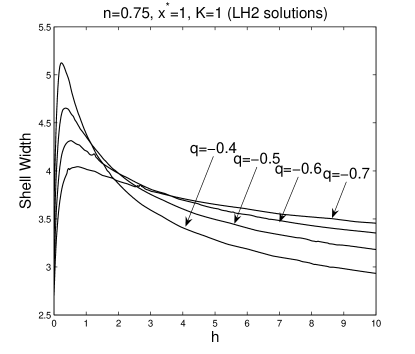
Figure 15: Shell width variation of LH2 solutions versus the magnetic parameter $h$ for different values of $q$ parameter. The shell width is defined as the distance from the void boundary to the place where the density is $e^{-1}$ of the peak density. The common parameters for these solutions are $n=0.75,\ x^{*}=1,\ K=1$.

7 Summary and Conclusions

In a general polytropic MHD formulation, we obtain novel self-similar void solutions for a magnetofluid under self-gravity and with quasi-spherical symmetry. For our MHD void solutions, the enclosed mass within the void boundary is zero and our solutions are valid from the void boundary outwards. We have carefully examined MHD and hydrodynamic behaviours near the void boundary and obtained complete asymptotic solutions in various parameter regimes. For clarity, we consider the situation of density being zero at the void boundary and other situations separately.

For the case of $\alpha^{*}=0$ at the void boundary, we derive novel LH1 solutions with $q>0$, for which the void boundary is also a critical curve, and LH2 solutions with $q<0$, for which the thermal pressure force becomes dominant approaching the void boundary. A random magnetic field must be present in order to construct LH1 solutions. Both LH1 and LH2 solutions have shell-type morphology in the density profile, whose peak density and the shell width are mainly determined by the values of the magnetic parameter $h$ and the parameter $q$. The shell width of the density profile expands with time also in a self-similar manner.

For the case of $\alpha^{*}\neq 0$ at the void boundary, the situation is quite different between the hydrodynamic and MHD cases. In hydrodynamic cases, asymptotic behaviours in the vicinity of void boundary depends on parameter $q$ and can be classified as Type-N ($q=0$) and Type-D ($q>0$). For the Type-D behaviour, the density at the void boundary diverges, and local diffusion process should occur. We systematically examined all these possibilities and present a few numerical solution examples. Our solutions are well compatible with previous self-similar solutions; for example, by setting $q=0$, our formulation reduces to self-similar solutions for a conventional polytropic gas (Lou & Wang 2007). Without magnetic field, for both Type-N and Type-D behaviours, the thermal pressure force dominates at the void boundary; actually Type-N solutions can be regarded as a natural extension of LH2 solutions in the regime of $q=0$, and Type-D solutions as a natural extension of LH2 solutions in the regime of $q>0$. Therefore, for all sensible void solutions in hydrodynamic framework, the thermal pressure is the dominant force at the void boundary. By including a random magnetic field, which is ubiquitous in astrophysical plasmas, the divergence at the void boundary appearing in the type-D behaviour can be removed, and the dominant force on the void boundary becomes the magnetic force.

Void solutions may go across the critical curve either smoothly or by an MHD shock and then merge into asymptotic solution (32) of finite density and velocity at large $x$. If void solutions do not encounter the critical curve, they generally merge into one kind of asymptotic expansion solutions at large $x$ with the velocity proportional to the radius. For $q<2/3$, void solutions merge into asymptotic free-expansion solutions, for which the thermal pressure force is negligible. For $q>2/3$, void solutions merge into asymptotic thermal-expansion solutions, for which the thermal pressure force is dominant. For $q=2/3$, void solutions merge into the Einstein-de Sitter solution, a semi-complete global exact solution. We are free to choose the position of void boundary $x^{*}$, the density on the void boundary $\alpha^{*}$ (or the density parameter $K$) and the downstream shock position $x_{\rm sd}$ to construct various void solutions with different asymptotic dynamic behaviours far from the void centre, including inflows, outflows, contraction and breeze for upstream solutions.

In this paper, we briefly discussed the case of $q=2/3$ and thus $\gamma=4/3$ for a relativistically hot gas (Goldreich & Weber 1980; Lou & Cao 2008; Cao & Lou 2009). One more parameter appears in the self-similar form of the equation of state denoted as $C$ in this case. We show solution examples of $C=1$. A more detailed study, including cases of $C\neq 1$ is forthcoming.

Finally, we provide examples of applications of our self-similar MHD void solutions. In principle, our solutions can be adapted to various astrophysical plasmas with a central cavity. The scale of a system can vary within the upper limit of neglecting the universe expansion. The input and output of energy can be approximated by properly choosing parameters $(n,\ \gamma,\ k)$. As more self-consistent solutions of an MHD problem usually require tremendous computational effort, our self-similar approach is valuable in conceptual modelling and in checking simulation results. We provide an application of our void solutions to the neutrino reheating mechanism for core-collapse supernovae and compare the dynamical results of self-similar solutions with previous numerical simulations. We find that our simplified model fits well with numerical simulations, suggesting that the self-similar approach is plausible and the exploding stellar envelope and the rebound shock do evolve in a self-similar manner. More specifically, we estimate that a rebound shock breaks out from the stellar photosphere $\sim 4000$ s after the core bounce, for a progenitor star of mass 25 M_⊙ and radius $\sim 10^{12}$ cm. We expect that, our general polytropic self-similar MHD solutions, coupled with radiative transfer processes, may offer physical insight for the rebound shock evolution of massive stars as well as on GRB-supernova associations. We also indicate potential applications of LH1 and LH2 void solutions, with shell-type morphology, on the shell-type supernova remnants as well as hot bubbles in the interstellar medium.

8 Acknowledgments

This research was supported in part by the Tsinghua Centre for Astrophysics, by the NSFC grants 10373009 and 10533020 and by the National Basic Science Talent Training Foundation (NSFC J0630317) at Tsinghua University, and by the SRFDP 20050003088 and 200800030071 and the Yangtze Endowment from the Ministry of Education at Tsinghua University. The kind hospitality of Institut für Theoretische Physik und Astrophysik der Christian-Albrechts-Universität Kiel is gratefully acknowledged.

Appendix A MHD shock jump conditions

MHD shocks can be constructed for self-similar solutions to cross the MSS. Despite discontinuities in pressure, mass density, temperature, magnetic field and velocity across the shock front, we require conservations of mass, radial momentum, MHD energy across a shock front in the comoving shock reference framework, respectively. They are

$$\big{[}\rho(u_{s}-u)\big{]}_{1}^{2}=0\ ,$$ (46)

$$\bigg{[}p+\rho(u_{s}-u)^{2}+\frac{<B_{t}^{2}>}{8\pi}\bigg{]}_{1}^{2}=0\ ,$$ (47)

$$\bigg{[}\frac{\rho(u_{s}-u)^{3}}{2}+\frac{\gamma p(u_{s}-u)}{(\gamma-1)}+\frac{<B_{t}^{2}>}{4\pi}(u_{s}-u)\bigg{]}_{1}^{2}=0\ ,$$ (48)

where $u_{s}$ is the shock travel speed in the laboratory framework of reference. Since we only consider the dominant transverse magnetic field parallel to the shock front in our theoretical model framework, the magnetic induction equation can be written as

$$\big{[}(u_{s}-u)^{2}<B_{t}^{2}>\big{]}_{1}^{2}=0\ .$$ (49)

The magnetic field average is made over a layer between $r$ and $r+dr$, and such average can still describe the discontinuity in the radial direction. Strictly speaking, the magnetic fields have weak radial components normal to the shock front. We presume that such radial components are extremely weak compared to the transverse components on large scales. In common with the conventional shock analysis (e.g. Zel’dovich & Raizer 1966, 1967), we use a pair of square brackets outside each expression enclosed to denote the difference between the upstream (subscript ‘1’) and downstream (superscript ‘2’) sides across a MHD shock front. Note that the definitions of the downstream and upstream sides are in the reference framework where the shock front is at rest, and the specific entropy increases from the upstream side to the downstream side. The sound parameter $k$ in transformation (6) is related to the polytropic sound speed and changes across a shock. We therefore relate upstream $k_{1}$ and downstream $k_{2}$ with a ratio factor $\lambda$ such that

$$k_{2}=\lambda^{2}k_{1}\ ,\quad\qquad h_{1}=h_{2}\ ,\quad\qquad x_{1}=\lambda x_{2}\ .$$ (50)

The latter two in condition (50) are for the jump of the magnetic energy density $<B_{t}^{2}>$ and the continuity of shock radius $r_{s}$ across the MHD shock front, which means while the dimensionless shock front $x_{\rm s}$ has different values across the shock, they correspond to the same shock front radius $r_{s}$. With the definition of $h$, $h_{1}=h_{2}$ actually means the transverse magnetic field is proportional to the mass density across the shock front, consistent with Dyson & Williams (1997). Using $h$ instead of $h_{1}$ and $h_{2}$ for the magnetic parameter and substituting equation (50) into MHD shock conditions (46)$-$(49), we obtain self-similar MHD shock conditions

$$\alpha_{1}(nx_{1}-v_{1})=\lambda\alpha_{2}(nx_{2}-v_{2})\ ,$$ (51)

$$\qquad C\alpha_{1}^{2-n+3nq/2}x_{1}^{2q}(nx_{1}-v_{1})^{q}$$

$$\qquad\quad+\alpha_{1}(nx_{1}-v_{1})^{2}+\frac{h\alpha_{1}^{2}x_{1}^{2}}{2}$$

$$\qquad\qquad=\lambda^{2}\bigg{[}C\alpha_{2}^{2-n+3nq/2}x_{2}^{2q}(nx_{2}-v_{2})^{q}$$

$$\qquad\qquad\quad+\alpha_{2}(nx_{2}-v_{2})^{2}+\frac{h\alpha_{2}^{2}x_{2}^{2}}{2}\bigg{]}\ ,$$ (52)

$$(nx_{1}-v_{1})^{2}+\frac{2\gamma}{(\gamma-1)}C\alpha_{1}^{1-n+3nq/2}$$

$$\qquad\times x_{1}^{2q}(nx_{1}-v_{1})^{q}+2h\alpha_{1}x_{1}^{2}$$

$$\qquad\quad=\lambda^{2}\bigg{[}(nx_{2}-v_{2})^{2}+\frac{2\gamma}{(\gamma-1)}C\alpha_{2}^{1-n+3nq/2}$$

$$\qquad\qquad\times x_{2}^{2q}(nx_{2}-v_{2})^{q}+2h\alpha_{2}x_{2}^{2}\bigg{]}\$$ (53)

in terms of the dimensionless reduced variables. Once we have $(x_{2},\ \alpha_{2},\ v_{2})$ on the downstream side of a shock, we can determine $(x_{1},\ \alpha_{1},\ v_{1})$ on the upstream side using MHD shock conditions $(\ref{equ181})-(\ref{equ183})$ (Wang & Lou 2008) or vice versa. In cases of $q=2/3$, there are only two independent relations among (51)$-$(53) (Lou & Cao 2008); therefore one may choose parameter $\lambda>0$ fairly arbitrarily, e.g. $\lambda=1$.

References

- [1] Arnal E. M., Mirabel I. F., 1991, A&A, 250, 171
- [2] Arnal E. M., 1992, A&A, 254, 305
- [3] Bian F.-Y., Lou Y.-Q., 2005, MNRAS, 363, 1315
- [4] Buras R., Janka T.-H., Rampp M., Kifonidis K., 2006, A&A, 457, 281
- [5] Campana S., Mangano V., Blustin A.J., Brown P., et al., 2006, Nature, 442, 1008
- [6] Cao Y., Lou Y.-Q., 2009, submitted
- [7] Cappa de Nicolau C. E., Niemela V. S., 1984, AJ, 89, 1398
- [8] Cappa de Nicolau C. E., Niemela V. S., Arnal E. M., 1986, AJ, 92, 1414
- [9] Cappa de Nicolau C. E., Niemela V. S., Dubner G. M., Arnal E. M., 1988, AJ, 96, 1671
- [10] Castor J., McCray R., Weaver R., 1975, ApJ, 200, L107
- [11] Chevalier R. A., 1997, ApJ, 488, 263
- [12] Chiueh T., Chou J.-K., 1994, ApJ, 431, 380
- [13] Colomb F. R., Dubner G. M., Giacani E. B., 1984, A&A, 130, 294
- [14] Crosthwaite L. P., Turner J. L., 2000, ApJ, 119, 1720
- [15] Dubner G. M., Niemela V. S., Purton C. R., 1990, AJ, 99, 857
- [16] Dyson J. E., Williams D. A., 1997, The Physics of The Interstellar Medium (Bristol and Philadelphia: Institute pf Physics Publishing)
- [17] Ferrière K., 1998, ApJ, 503, 700
- [18] Ferrière K., 2001, Rev. Mod. Phys., 73, 1031
- [19] Franco G. A. P., 2002, MNRAS, 331, 474
- [20] Franco J., Kurtz S., Hofner P., Testi L., García-Segura G. et al., 2000, ApJ, 542, L143
- [21] Gahm G. F., Gebeyehu M., Lindgren M., Magnusson P., Modigh P., Nordh H. L., 1990, A&A, 228, 477
- [22] Goldreich P., Weber S. V., 1980, ApJ, 238, 991
- [23] Hu R.-Y., Lou Y.-Q., 2008a, MNRAS, 390, 1619
- [24] Hu R.-Y., Lou Y.-Q., 2008b, AIP Proceedings 1065 of 2008 Nanjing Gamma-Ray Bursts Conference, eds. Y. F. Huang, Z. G. Dai, B. Zhang, Nanjing University, p 310
- [25] Hu R.-Y., Lou Y.-Q., 2009, MNRAS (2009arXiv:0902.3111) in press
- [26] Janka H.-T., Hillebrant W., 1989, A&AS, 78, 375
- [27] Janka H.-T., Müller E., 1995, ApJ, 448, L109
- [28] Janka H.-T., Müller E., 1996, A&A, 306, 167
- [29] Janka H.-T., Langanke K., Marek A., Martínez-Pinedo G., Müller B., 2007, Phys. Reports., 442, 38
- [30] Janka H.-T., Andreas M., Müller B., Scheck L., 2008, AIP Conference Proceedings, 983, 369
- [31] Jiang Y. F., Lou Y.-Q., 2009, submitted
- [32] Jordan D. W., Smith P., 1977, Nonlinear Ordinary Differential Equations (Oxford: Oxford University Press)
- [33] Liebendörfer M., Rampp M., Janka T.-H., Mezzacappa A., 2005, ApJ, 620, 840
- [34] Lou Y.-Q., 1993, ApJ, 414, 656
- [35] Lou Y.-Q., Cao Y., 2008, MNRAS, 384, 611
- [36] Lou Y.-Q., Jiang Y. F., Jin C. C., 2008, MNRAS, 386, 835
- [37] Lou Y.-Q., Jiang Y. F., 2008, MNRAS, 391, L44
- [38] Lou Y.-Q., Wang W.-G., 2006, MNRAS, 372, 885
- [39] Lou Y.-Q., Wang W.-G., 2007, MNRAS, 378, L54
- [40] Lou Y.-Q., Zhai X., ApSS, 2009, submitted
- [41] Mazzali P. A., et al., 2008, Science, 223, L109
- [42] McKee C., Tan J. C., 2002, Nature, 416, 59
- [43] McKee C. F., van Buren D., Lazareff B., 1984, ApJ, 278, L115
- [44] McNamara B. R., Nulsen P. E. J., Wise M. W., Rafferty D. A., Carilli C., Sarazin C. L., Blanton E. L., 2005, Nature, 433, 45
- [45] Meyer F., 1997, MNRAS, 285, L11
- [46] Myers, P. C., 1998, ApJ, 496, L109
- [47] Niemela V. S., Cappa de Nicolau C. E., 1991, A&A, 101, 572
- [48] Osorio M., Lizano S., D’Alessio P., 1999, ApJ, 525, 808
- [49] Press W. H., Flannery B. P., Teukolsky S. A., Vetterling W., 1986, Numerical Recipes (Cambridge: Cambridge University Press)
- [50] Riegler G. R., Agrawal P. C., Gull S. F., 1980, ApJ, 235, L71
- [51] Shu F. H., 1977, ApJ, 214, 488
- [52] Shu F. H., Adams F. C., Lizano S., 1987, Annu. Rev. Astron. Astrophys., 25, 23
- [53] Shu F. H., Lizano S., Galli D., Canto J., Laughlin G., 2002, ApJ, 580, 969
- [54] Suto Y., Silk J., 1988 ApJ, 326, 527
- [55] Soderberg A. M., Berger E., Page K. L., Schady P., Parrent J., et al., 2008, Nature, 453, 469
- [56] Tsai J. C., Hsu J. J. L., 1995, ApJ, 448, 774
- [57] Wallace B. J., Landecker T. L., Taylor A. R., 1994, A&A, 286, 565
- [58] Wang W.-G., Lou Y.-Q., 2007, ApSS, 311, 363
- [59] Wang W.-G., Lou Y.-Q., 2008, ApSS, 315, 135
- [60] Weaver R., McCray R., Castor J., 1977, ApJ, 218, 377
- [61] Weber E.J., Davis L. Jr., 1967, ApJ, 148, 217
- [62] Wolf S., Launhardt R., Henning T., 2003, ApJ, 592, 233
- [63] Yahil A., 1983, ApJ, 265, 1047
- [64] Yu C., Lou Y.-Q., 2005, MNRAS, 364, 1168
- [65] Yu C., Lou Y.-Q., Bian F.-Y., Wu Y., 2006, MNRAS, 370, 121
- [66] Zel’dovich Ya. B., Novikov I. D., 1971, Stars and Relativity C Relativistic Astrophysics, Vol. 1 (Chicago: The University of Chicago Press)
- [67] Zel’dovich Ya. B., Raizer Yu. P., 1966, Elements of Gas dynamics and the Classical Theory of Shock Waves (New York: Academic Press)
- [68] Zel’dovich Ya. B., Raizer Yu. P., 1967, Physics of Shock Waves and High-Temperatures Hydrodynamic Phenomena (New York: Academic Press)