Chiral Extrapolations of light resonances from dispersion relations and Chiral Perturbation Theory

Abstract:

We review our recent study of the pion mass dependence of the $\rho$ and $\sigma$ resonances, generated from one-loop $SU(2)$ Chiral Perturbation Theory (ChPT) with the Inverse Amplitude Method (IAM) which was modified to properly account for the Adler zero. The method is based on analyticity, elastic unitarity and ChPT at low energies, thus yielding the pion mass dependence of the resonance pole positions from the ChPT series up to a given order. We find that the $\rho\pi\pi$ coupling constant is almost $m_{\pi}$ independent and that our prediction compare well with some recent lattice results for the $\rho$ mass. These findings may be relevant for studies of the meson spectrum and form factors on the lattice.

1 Introduction

Light hadron spectroscopy at low energies lies beyond the realm of perturbative QCD. Although lattice QCD provides, in principle, a rigorous way to extract non–perturbative quantities from QCD, current lattice results are typically still obtained for relatively high quark masses. Thus, in order to make contact with experiment, appropriate extrapolation formulas need to be derived. This is typically done by using Chiral Perturbation Theory (ChPT)[1], which provides a model independent description of the dynamics of the lightest mesons, namely, the pions, kaons and etas, which are identified with the Goldstone Bosons (GB) associated to the QCD spontaneous Chiral Symmetry breaking. Hence, ChPT is built out of only those fields, as a low energy expansion of a Lagrangian whose terms respect all QCD symmetries, and in particular its symmetry breaking pattern. Actually, this chiral expansion becomes a series in momenta and meson masses, generically $O(p^{2}/\Lambda^{2})$, when taking into account systematically the small quark masses of the three lightest flavors that can be treated perturbatively. The chiral expansion scale is $\Lambda\equiv 4\pi f_{\pi}$, where $f_{\pi}$ denotes the pion decay constant. ChPT is renormalized order by order by absorbing loop divergences in the renormalization of parameters of higher order counterterms, known as low energy constants (LEC), which are the coefficients of the energy and mass expansion, so that they have no quark mass dependence. Their values depend on the specific QCD dynamics, and have to be determined either from experiment or from lattice QCD.

The relevant remark for us is that, thanks to the fact that ChPT has the same symmetries as QCD and that it couples to different kind of currents through the same pattern, the ChPT expansion provides a systematic and model independent description of how the observables depend on some QCD parameters, like the quark masses, and this can be implemented systematically up to the desired order in the ChPT expansion.

We review here our recent derivation of a modified version of the IAM [2] based on dispersion theory, unitarity and ChPT to next–to–leading order (NLO), which also accounts properly for the Adler zero. Within this approach we are able to predict the quark mass dependence of the $\sigma$ and $\rho$ mesons [3], thus providing an explicit representation of the LECs appearing in the ChPT analysis of the vector meson mass of Refs. [4, 5].

In this work we focus on the two lightest resonances of QCD, the $\rho$ and the $\sigma$. It is therefore enough to work with the two lightest quark flavors $u,d$ in the isospin limit with a mass $\hat{m}=(m_{u}+m_{d})/2$. Since $m_{\pi}$ is given by $m_{\pi}^{2}\sim\hat{m}+...$ [1], studying the $\hat{m}$ dependence is equivalent to study the $m_{\pi}$ dependence.

2 Unitarization and dispersion theory

The $\sigma$ and $\rho$ resonances appear as poles on the second Riemann sheet of the $(I,J)=(0,0)$ and $(1,1)$ $\pi\pi$ scattering partial waves of isospin $I$ and angular momentum $J$, respectively. Unitarity implies for these partial waves, and physical values of $s$ below inelastic thresholds, that

$${\mbox{Im}\,}t(s)=\sigma(s)|t(s)|^{2}\;\;\Rightarrow\;\;{\mbox{Im}\,}\frac{1}{t(s)}=-\sigma(s),\qquad{\rm with}\quad\sigma(s)=2p/\sqrt{s},$$ (1)

where s is the Mandelstam variable and $p$ is the center of mass momentum. Consequently, the imaginary part of the inverse amplitude is known exactly. Hoewever, ChPT ampitudes, being an expansion $t\simeq t_{2}+t_{4}+\cdots$, with $t_{k}=O(p^{k})$, can only satisfy Eq. (1) perturbatively

$${\mbox{Im}\,}t_{2}(s)=0,\;\;\;{\mbox{Im}\,}t_{4}(s)=\sigma(s)|t_{2}(s)|^{2},\;\;\dots\quad\Rightarrow\quad{\mbox{Im}\,}\frac{t_{4}(s)}{t_{2}^{2}(s)}=\sigma(s),$$ (2)

and cannot generate poles. Therefore the resonance region lies beyond the reach of standard ChPT. This region however, can be reached combining ChPT with dispersion theory either for the amplitude [6] or for the inverse amplitude through the IAM [7, 8, 9].

Here we review our recent derivation [2] of a modified IAM formula to properly account for the Adler zero region. The main ingredient is a dispersion relation for the inverse amplitude, whose analytic structure consist on a right cut from $s=4m_{\pi}^{2}$ to $s=\infty$, a left cut from $s=-\infty$ to $s=0$, and possible poles comming from zeros of the amplitude. Indeed, for the scalar waves the amplitude vanishes at the so called Adler zero, $s_{A}$, that lies in the real axis below threshold, thus within the ChPT region of applicability. Its position can be approximated from ChPT, i.e., $s_{A}=s_{2}+s_{4}+\cdots$, where $t_{2}$ vanishes at $s_{2}$, $t_{2}+t_{4}$ at $s_{2}+s_{4}$, etc.

We now write a once substracted dispersion relation for the inverse amplitude, where the substraction point has been chosen to be the Adler zero, $s_{A}$:

$$\frac{1}{t(s)}=\frac{s-s_{A}}{\pi}\int_{RC}ds^{\prime}\frac{{\mbox{Im}\,}1/t(s^{\prime})}{(s^{\prime}-s_{A})(s^{\prime}-s)}+LC(1/t)+PC(1/t),$$ (3)

where $LC$ stands for a similar integral over the left cut and $PC$ stands for the contribution of the pole at the Adler zero, which reads:

$$PC(1/t)=-(s-s_{A})\operatorname*{Res}_{s^{\prime}=s_{A}}\left(\frac{1/t(s^{\prime})}{(s^{\prime}-s)(s^{\prime}-s_{A})}\right)=\frac{1}{t^{\prime}(s_{A})(s-s_{A})}-\frac{t^{\prime\prime}(s_{A})}{2t^{\prime}(s_{A})^{2}}.$$

The different terms in Eq. (3), can be evaluated in the following way:

• The right cut can be exactly evaluated taking into account the elastic unitarity condition Eqs. (1), (2), ${\mbox{Im}\,}1/t(s^{\prime})=-\sigma(s^{\prime})=-{\mbox{Im}\,}t_{4}(s^{\prime})/t_{2}^{2}(s^{\prime})$, for $s^{\prime}\in(4m_{\pi}^{2},\infty)$.

• The pole contribution only involves amplitude derivatives evaluated at the Adler zero, which is a low energy point, so they can be can be safely approximated with ChPT.

• The left cut, which is $1/(s^{\prime}-s)$ suppressed for $s$ values near the physical region, is weighted at low energies, so it is appropiate to approximate it with ChPT.

• Finally, in the cut contributions we approximate $(s-s_{A})/(s^{\prime}-s_{A})\simeq(s-s_{2})/(s^{\prime}-s_{2})$, which is its LO chiral expansion and a remarkably good approximation as long as $s^{\prime}$ is is sufficiently far from $s_{2}$ and $s_{A}$, which is indeed the case for the cut integrals.

Altogether we are able to write Eq. (3) as

$$\frac{1}{t(s)}\simeq\underbrace{-RC(t_{4}/t_{2}^{2})-LC(t_{4}/t_{2}^{2})}_{-t_{4}(s)/t_{2}^{2}(s)+PC(t_{4}/t_{2}^{2})}+PC(1/t)=-\frac{t_{4}(s)}{t_{2}^{2}(s)}+PC(t_{4}/t_{2}^{2})+PC(1/t),$$ (4)

where we have taken into account that a once subtracted dispersion relation can be written for $t_{4}/t_{2}^{2}$, the substraction point being $s_{2}$:

$$\frac{t_{4}(s)}{t_{2}^{2}(s)}=\frac{s-s_{2}}{\pi}\int_{RC}ds^{\prime}\frac{{\mbox{Im}\,}\,t_{4}(s^{\prime})/t_{2}^{2}(s^{\prime})}{(s^{\prime}-s_{2})(s^{\prime}-s)}+LC(t_{4}/t_{2}^{2})+PC(t_{4}/t_{2}^{2}),$$ (5)

where $PC(t_{4}/t_{2}^{2})$ stands for the contribution of the triple pole at $s_{2}$. From Eq. (4) one easily arrives at the modified IAM (mIAM) formula [2]:

$$t^{mIAM}(s)\simeq\frac{t_{2}^{2}(s)}{t_{2}(s)-t_{4}(s)+A(s)},\quad A(s)=t_{4}(s_{2})-\frac{(s_{2}-s_{A})(s-s_{2})}{s-s_{A}}\Big{(}t^{\prime}_{2}(s_{2})-t^{\prime}_{4}(s_{2})\Big{)}.$$ (6)

The standard IAM formula is recovered for $A(s)=0$, which holds exactly for all partial waves except the scalar ones. In the original IAM derivation [7, 8] $A(s)$ was neglected, since it formally yields a NNLO contribution and is numerically very small, except near the Adler zero, where it diverges. However, if $A(s)$ is neglected, the IAM Adler zero occurs at $s_{2}$, correct only to LO, it is a double zero instead of a simple one, and a spurious pole of the amplitude appears close to the Adler zero on both the first and second sheet. All of these caveats are removed with the mIAM, Eq. (6). The differences in the physical and resonance region between the IAM and the mIAM are less than 1%. However, as we will see, for large $m_{\pi}$ the $\sigma$ poles appear as two virtual poles on the second sheet below threshold, one of them moving towards zero and approaching the Adler zero region, where the IAM fails. Thus, we will use for our calculations the mIAM, although it is only relevant for the mentioned second $\sigma$ pole, and only when it is very close to the spurious pole.

In summary, there are no model dependences in the approach, but just approximations to a given order in ChPT. Let us remark that, in our derivation, ChPT has been used always at low energies to evaluate parts of a dispersion relation, whose elastic unitarity cut is taken into account exactly. Thus, the IAM formula is reliable up to energies where inelasticities become important, even though ChPT does not converge at those energies, because ChPT is not being used there. This argument also holds when the $\sigma$ moves near threshold, because the Adler zero, which is the point where ChPT is used, is still at low energies far away from the pole. Note that the virtual pole that goes down in energies is on the second sheet, so does not prevent the use ChPT at the Adler zero, on the first sheet. Remarkably, the simple formula of the elastic mIAM, Eq.(6), (or the standard IAM one), while reproducing the ChPT expansion at low energies, is also able to generate both the $\rho$ and $\sigma$ resonances with values of the LECs compatible with standard ChPT [9]. In other words, the IAM generates the poles [8] associated to these resonances in the second Riemann sheet. The fact that resonances are not introduced by hand but generated from first principles and data, is relevant because the existence and nature of scalar resonances is the subject of a long-lasting intense debate.

To be precise, the IAM, when reexpanded, reproduces the ChPT series up to the order to which the input amplitude was evaluated and, in particular, the quark mass dependence agrees with that of ChPT up to that order. A few of the higher order terms are produced correctly by the unitarization but not the complete series— for a discussion of this issue for the scalar pion form factor see Ref.[10]. However, the formalism just described still provides us with a fair estimate of the quark mass dependence of the resonance properties.

3 Results

By changing $m_{\pi}$ in the amplitudes we see how the poles generated with the IAM evolve. We will use the LECs values $10^{3}l^{r}_{3}=0.8\pm 3.8$ and $10^{3}l^{r}_{4}=6.2\pm 5.7$ from [1] and fit the mIAM to data up to the resonance region to find $10^{3}l^{r}_{1}=-3.7\pm 0.2$ and $10^{3}l^{r}_{2}=5.0\pm 0.4$. These LECs are evaluated at $\mu=770$ MeV.

The values of $m_{\pi}$ considered should fall within the ChPT range of applicability and allow for some elastic $\pi\pi$ regime below $K\bar{K}$ threshold. Both criteria are satisfied if $m_{\pi}\leq 500$ MeV, since $SU(3)$ ChPT still works with such kaon masses, and because for $m_{\pi}\simeq 500$ MeV, the kaon mass becomes $\simeq 600$, leaving 200 MeV of elastic region. Of course, we expect higher order corrections, which are not considered here, to become more relevant as $m_{\pi}$ is increased. Thus, our results become less reliable as $m_{\pi}$ increases due to the $O(p^{6})$ corrections which we have neglected

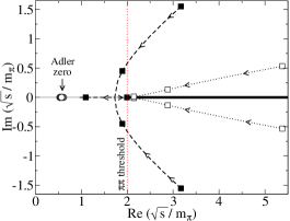
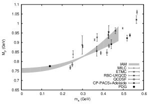
Figure 1: Left: Movement of the $\sigma$ (dashed lines) and $\rho$ (dotted lines) poles for increasing $m_{\pi}$ (direction indicated by the arrows) on the second sheet. The filled (open) boxes denote the pole positions for the $\sigma$ ($\rho$) at pion masses $m_{\pi}=1,\ 2,$ and $3\times m_{\pi}^{\rm phys}$, respectively. For $m_{\pi}=3m_{\pi}^{\rm phys}$ three poles accumulate in the plot very near the $\pi\pi$ threshold. Note that all poles are always far enough from the Adler zero (circles). Right: Comparison of our results for the $M_{\rho}$ dependence on $m_{\pi}$ with some recent lattice results from [11]. The grey band covers only the error coming from the LECs uncertainities.

Fig. 1 (left) shows the evolution of the $\sigma$ and $\rho$ pole positions as $m_{\pi}$ is increased. In order to see the pole movements relative to the two pion threshold, which is also increasing, all quantities are given in units of $m_{\pi}$, so the threshold is fixed at $\sqrt{s}=2$. Both poles moves closer to threshold and they approach the real axis. The $\rho$ poles reach the real axis as the same time that they cross threshold. One of them jumps into the first sheet and stays below threshold in the real axis as a bound state, while its conjugate partner remains on the second sheet practically at the very same position as the one in the first. In contrast, the $\sigma$ poles go below threshold with a finite imaginary part before they meet in the real axis, still on the second sheet, becoming virtual states. As $m_{\pi}$ is increased further, one of the poles moves toward threshold and jumps through the branch point to the first sheet and stays in the real axis below threshold, very close to it as $m_{\pi}$ keeps growing. The other $\sigma$ pole moves down in energies further from threshold and remains on the second sheet. This analytic structure, with two very asymmetric poles in different sheets for a scalar wave, could be a signal of a prominent molecular component [12, 13], at least for large pion masses. Similar pole movements have been also found within quark models [14] and in finite density analysis [15].

In Fig. 2 (left) we show the $m_{\pi}$ dependence of $M_{\rho}$ and $M_{\sigma}$ (defined from the pole position $\sqrt{s_{pole}}=M-i\Gamma/2$), normalized to their physical values. The bands cover the LECs uncertainties. We see that both masses grow with $m_{\pi}$, but $M_{\sigma}$ grows faster than $M_{\rho}$. Below $m_{\pi}\simeq 330$ MeV we only show one line because the two conjugate $\sigma$ poles have the same mass. Above 330 MeV, these two poles lie on the real axis with two different masses. The heavier pole goes towards threshold and around $m_{\pi}\simeq 465$ MeV moves into the first sheet. Note also that the $m_{\pi}$ dependence of $M_{\sigma}$ is much softer than suggested in [16], shown as the dotted line, which in addition does not show the two virtual poles.

In the right panel of Fig. 2 we show the $m_{\pi}$ dependence of $\Gamma_{\rho}$ and $\Gamma_{\sigma}$ normalized to their physical values, where we see that both widths become smaller. We compare this decrease with the expected reduction from phase space as the resonances approach the $\pi\pi$ threshold. We find that $\Gamma_{\rho}$ follows very well this expected behavior, which implies that the $\rho\pi\pi$ coupling is almost $m_{\pi}$ independent. In contrast $\Gamma_{\sigma}$ shows a different behavior from the phase space reduction expectation. This suggest a strong $m_{\pi}$ dependence of the $\sigma$ coupling to two pions, necessarily present for molecular states [13, 17].

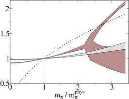
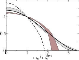
Figure 2: $m_{\pi}$ dependence of resonance masses (left) and widths (right) in units of the physical values. In both panels the dark (light) band shows the results for the $\sigma$ ($\rho$). The width of the bands reflects the uncertainties induced only from the uncertainties in the LECs. The dotted line shows the $\sigma$ mass dependence estimated in Ref. [16]. The dashed (continuous) line shows the $m_{\pi}$ dependence of the $\sigma$ ($\rho$) width from the change of phase space only, assuming a constant coupling of the resonance to $\pi\pi$.

Fig. 1 (right) shows our results for the $\rho$ mass (here defined as the point where the phase shift crosses $\pi/2$, except for those $m_{\pi}$ values where the $\rho$ becomes a bound state, where it is defined then from the pole position) dependence on $m_{\pi}$ compared with some recent lattice results [11], where we also quote the PDG value for the $\rho$ mass. Taking into account the incompatibilities within errors between different lattice colaborations, we find a qualitaive good agreement with the lattice resuts. Also, we have to take into account that the $m_{\pi}$ dependence in our approach is correct only up to NLO in ChPT, and we expect higher order corrections to be important for large pion masses.

4 Summary

We have reviewed our derivation of a modified version of the IAM [2], which is derived from the first principles of analyticity, unitarity, and ChPT at low energies and has the correct behaviour around the Adler zero. It is able to generate the $\sigma$ and $\rho$ resonance poles without any a priori assumptions, and yields the correct dependence on the pion mass up to NLO in ChPT. We have predicted the evolution of the resonance pole positions with increasing pion mass [3] and have seen that both resonances become bound states. We have also shown that the $\rho\pi\pi$ coupling constant is almost $m_{\pi}$ independent and we have found a qualitative agreement with some lattice results for the $\rho$ mass evolution with $m_{\pi}$. These findings might be relevant for studies of the meson spectrum and form factors—see Ref. [18]—on the lattice.

References

- [1] S. Weinberg, Physica A96 (1979) 327. J. Gasser and H. Leutwyler, Annals Phys. 158 (1984) 142; Nucl. Phys. B 250 (1985) 465.
- [2] A. Gómez Nicola, J.R. Peláez and G. Ríos, Phys. Rev. D 77 (2008) 056006.
- [3] C. Hanhart, J. R. Pelaez and G. Rios, Phys. Rev. Lett. 100, 152001 (2008)
- [4] P. C. Bruns and U.-G. Meißner, Eur. Phys. J. C 40 (2005) 97
- [5] D. Djukanovic, J. Gegelia, A. Keller and S. Scherer, [arXiv:hep-ph/0902.4347].
- [6] I. Caprini et al., Phys. Rev. Lett. 96 (2006) 132001
- [7] T. N. Truong, Phys. Rev. Lett. 61 (1988) 2526. Phys. Rev. Lett. 67, (1991) 2260; A. Dobado et al., Phys. Lett. B235 (1990) 134.
- [8] A. Dobado and J. R. Peláez, Phys. Rev. D 47 (1993) 4883; Phys. Rev. D 56 (1997) 3057.
- [9] F. Guerrero and J. A. Oller, Nucl. Phys. B 537 (1999) 459 [Erratum-ibid. B 602 (2001) 641]. J. R. Peláez, Mod. Phys. Lett. A 19, 2879 (2004) A. Gómez Nicola and J. R. Peláez, Phys. Rev. D 65 (2002) 054009 and AIP Conf. Proc. 660 (2003) 102. [hep-ph/0301049].
- [10] J. Gasser and U.-G. Meißner, Nucl. Phys. B 357 (1991) 90.
- [11] Ph. Boucaud et al. [ETM Collaboration], Phys. Lett. B 650, 304 (2007) C. Allton et al. [RBC and UKQCD Collaborations], Phys. Rev. D 76, 014504 (2007) C. W. Bernard et al.,Phys. Rev. D 64, 054506 (2001) C. R. Allton et al.Phys. Lett. B 628, 125 (2005) M. Gockeler et al.[QCDSF Collaboration],
- [12] D. Morgan, Nucl. Phys. A 543 (1992) 632; D. Morgan and M. R. Pennington, Phys. Rev. D 48 (1993) 1185.
- [13] V. Baru et al., Phys. Lett. B 586 (2004) 53.
- [14] E. van Beveren et al., AIP Conf. Proc. 660, 353 (2003); Phys. Rev. D 74, 037501 (2006).
- [15] D. Fernandez-Fraile, A. Gomez Nicola and E. T. Herruzo, Phys. Rev. D 76, 085020 (2007)
- [16] T. E. Jeltema and M. Sher, Phys. Rev. D 61 (2000) 017301
- [17] S. Weinberg, Phys. Rev. 130, 776 (1963); Y. Kalashnikova et al., Eur. Phys. J. A 24 (2005) 437.
- [18] F. K. Guo, C. Hanhart, F. J. Llanes-Estrada and U. G. Meissner, [arXiv:hep-ph/0812.3270].