Probing clustering features around Cl 0024+17

Abstract

I present a spatial analysis of the galaxy distribution around the cluster Cl 0024+17. The basic aim is to find the scales where galaxies present a significant deviation from an inhomogeneous Poisson statistical process. Using the generalization of the Ripley, Besag, and the pair correlation functions for non-stationary point patterns, I estimate these transition scales for a set of 1,000 Monte Carlo realizations of the Cl 0024+17 field, corrected for completeness up to the outskirts. The results point out the presence of at least two physical scales in this field at $31.4^{\prime\prime}$ and $112.9^{\prime\prime}$. The second one is statistically consistent with the dark matter ring radius ($\sim 75^{\prime\prime}$) previously identified by Jee et al. (2007). However, morphology and anisotropy tests point out that a clump at $\sim 120^{\prime\prime}$ NW from the cluster center could be the responsible for the second transition scale. These results do not indicate the existence of a galaxy counterpart of the dark matter ring, but the methodology developed to study the galaxy field as a spatial point pattern provides a good statistical evaluation of the physical scales around the cluster. I briefly discuss the usefulness of this approach to probe features in galaxy distribution and N-body dark matter simulation data.

1 Introduction

Galaxy clusters are the largest virialized structures in the universe. These systems are composed of three components behaving differently during collisions: galaxies, hot gas and dark matter. While the hot intergalactic gas presents strong eletromagnetic interactions during clusters enconteurs, both dark matter and galaxies are predicted to be collisioness, see e.g. [18]. Hence, clusters are important laboratories for studying the dynamics of the different kinds of matter in the universe. Indeed, galaxy clusters are themselves the result of several mergers of smaller groups of galaxies, see e.g. [10], a process still ongoing in many systems like, for instance, the so-called ’Bullet Cluster’ (1E 0657-56) [[17, 6]], and other clusters like Cl 0152-1357 and MS 1054, see [14, 15]. Also, cluster Cl 0024+17 has been a target of many studies since its discovery by [12]. This is an intermediate-redshift system (z=0.395) with both weak and strong lensing [25, 5, 7]. There are several indications that this cluster, an apparently relaxed system, is actually the portrait of a collision of two clusters, along our line of sight [8, 9, 20, 26, 16]. The weak lensing analysis presented by [16] shows a ring-like structure in the projected matter distribution at $r\sim 75^{\prime\prime}$ ($\sim$ 0.4 Mpc), surrounding a soft, dense core at $r\leq 50^{\prime\prime}$. The authors interpret this substructure as the result of a high-speed line-of-sight collision of two massive clusters $\sim$1-2 Gyr ago. An interesting question in this context refers to the behaviour of the galaxy component with respect to dark matter. In the case of the Bullet Cluster, Cl 0152-1357 and MS 1054-0321, the distribution of galaxies follows dark matter quite well [17, 6, 14, 15]. However, the recent work of [21], based on the 2D distribution of galaxies, suggests that the ringlike structure observed in dark matter measurements is not seen in the projected two-dimensional galaxy distribution.

In the present work, I introduce an alternative approach to probe both in radial and angular coordinates the projected galaxy distribution around galaxy clusters, and applied it to the case of Cl 0024+17. The basic aim is to find the scales where galaxies present a significant deviation from an inhomogeneous Poisson statistical process and compare that to the dark matter ring radius and the secondary clump present in the field.

2 Galaxy Sample

The sample of galaxies around Cl 0024+17 used in this work is taken from the catalog of Czoske et al. (2001). This corresponds to 295 galaxies in the range $0.37<z<0.41$, the most probable cluster members in the $\sim 0.3^{\circ}\times 0.3^{\circ}$ field. The center of the cluster was chosen to be the geometric center of the dark matter ring, see [16]. Distance $r$ for each galaxy was calculated from their equatorial coordinates, in arcsecs. Since the completeness of the sample varies from $>$80% at the cluster center to $<$50% in the outer regions, the catalog was corrected through 1,000 Monte Carlo realizations of the sample. This was done following approximately the completeness variation map of [8], adopting a procedure similar to [21]. One example of such realizations is presented in Figure 1, where black points are taken from the simulation and green points are the real galaxies from [8]. The background in this figure is a density map based on the void distance from each point with respect to a fine grid [3, 1]. This is just introduced to illustrate how the simulations fill the empty cells left by the original sample.

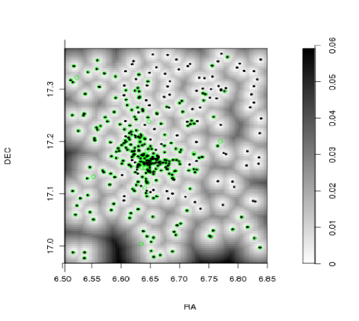
Figure 1: Simulated + real field on a void distance map. Simulated and real points are in black and green, respectively. The background is a density image built from the void distance matrix from each point with respect to a fine grid.

3 Methodology

3.1 Spatial Point Patterns

Galaxy distribution around Cl 0024+17 is the point pattern we want to probe. In statistical theory, a spatial point pattern (SPP) ${\bf x}=\{x_{1},...,x_{n}\}$ is simply a collection of points $x_{i}$ in some bounded area, and interpreted as a realization of a more generic point process ${\bf X}$. Analysis and modelling of SPP is a challenging topic in modern spatial spatistics. The mathematical theory was first developed to solve various problems where it is sensible to model the locations of events as random, [13]. Recently, statistical theory has made many developments with respect to SPP analysis. One of these advances is related to achievements in the study of nonstationary processes. Statistical stationarity (or homogeneity) means that the distribution of the point process is invariant under translations. This implies that the intensity $\lambda$, i.e. the expected number of points per unit area of the SPP, is constant. Nonstationarity, otherwise, allows for deterministic local variation of the intensity:$\lambda\rightarrow\lambda(u)$, where $u$ is a given location on the SPP. This is the case we are interested in this work, since galaxy distribution in the sampling window around the cluster is obviously inhomogeneous.

3.2 Ripley K-function

In spatial statistics, Ripley K-function [23] is a classical tool to analyse SPP. It is defined as the expected number of events within the distance $r$ of any given point divided by the intensity $\lambda$. The K-function, being a measure of the distribution of the inter-point distances,captures the spatial dependence between different regions of a SPP. Mathematically, the inhomogeneous K-function is defined as

$$K_{inhom}(r)={\rm E}\left[{1\over\lambda(u)}\sum_{x_{j}\in{\bf\rm X}}{1\over\lambda(x_{j})}{\bf 1}\{0<||u-x_{j}||\leq r\}~{}|~{}u\in{\bf\rm X}\right].$$ (1)

Thus, $\lambda(u)K(r)$ is the expected total ’weight’ of all random points within a distance $r$ of the point $u$, where the weight of a point $x_{i}$ is $1/\lambda(x_{i})$ [2], and for a Poisson process with intensity function $\lambda(u)$, the K-function reduces to $K_{inhom}=\pi r^{2}$.

A standard computational estimator of K is given by

$$\hat{K}_{inhom}(r)={1\over area(W)}\sum_{i}\sum_{j\neq i}{{\bf 1}\{||x_{i}-x_{j}||\leq r\}\over\hat{\lambda}(x_{i})\hat{\lambda}(x_{j})}e(x_{i},x_{j};r),$$ (2)

where $e(x_{i},x_{j};r)$ is an edge correction weight, $W$ is the observational window, and $\hat{\lambda}(u)$ is an estimate of the intensity function $\lambda(u)$.

Although the K-function is the classical tool to probe SPP, modern spatial statistics rarely uses K(r), but rather its variant, the L-function as introduced by [4]. In the planar case, the L-function estimator is defined as

$$\hat{L}_{inhom}(r)=\sqrt{{\hat{K}_{inhom}(r)\over\pi}}.$$ (3)

The advantage of using $L(r)$ is that it is always proportional to $r$, and in the Poisson case $L(r)=r$, [13]. Thus, $L(r)-r>0$ indicates clustering with respect to a Poisson process.

In this work, the L-function was applied to the galaxy distribution around Cl 0024+17 using the estimation algorithms provided in the library spatstat, developed by [3], and running under the R statistical package (www.cran.r-project.org). The edge correction used here is implemented in the tasks Kinhom and Linhom. It is briefly described in the next.

3.3 Edge Corrections

Edge corrections are used to correct biases in the estimation of K(or L)-function due to the loss of information near to the boundary of $W$. In this work, I have applied the following edge correction:

$$e(x_{i},x_{j};r)={{\bf 1}(b_{i}>r)\over{\sum_{j}{\bf 1}(b_{j}>r){1\over\lambda(x_{j})}}},$$ (4)

where $b_{i}$ is the distance from $x_{i}$ to the boundary of the window $W$. Among other options available in spatstat, this weighting function is considered the most computationally and statistically efficient when there are large numbers of points, see [2].

3.4 Intensity estimator $\hat{\lambda}(u)$

Finally, there remains the question of how to estimate the intensity function $\lambda(u)$. This is estimated using a ‘leave-one-out’ kernel smoother, as described in [2]. The estimate $\hat{\lambda}(x_{i})$ is computed by removing $x_{i}$ from the point pattern, then applying a Gaussian kernel smoothing to the remaining points, and finally evaluating the smoothed intensity at $x_{i}$ (in this work we set the kernel width equal to $30^{\prime\prime}$). This estimator is also included in Kinhom and Linhom.

4 Analysis of Cl 0024+17

I have used the routine Linhom to probe the galaxy distribution around Cl 0024+17. For each MC realization of this field, I found the scales where clustering weakens towards an inhomogeneous Poisson process. In Figure 1, regions above the line $L(r)=r$ describes clustered distribution of points. To test the null hypothesis of an inhomogeneous Poisson process I also plot in this figure the 95% envelopes computed from $M$ independent simulations of this process, with the same intensity as the galaxy field, i.e., $\hat{L}^{(j)}(r)$ for $j=1,...,M$. The upper and lower envelopes of these simulated curves are

$$\hat{L}^{lower}(r)=\min_{j}\hat{L}^{(j)}(r)$$ (5)

$$\hat{L}^{upper}(r)=\max_{j}\hat{L}^{(j)}(r).$$ (6)

If data come from a Poisson process, then $\hat{L}(r)$ and $\hat{L}^{(1)}(r)$,…,$\hat{L}^{(M)}(r)$ are statistically equivalent and independent, so the probability that $\hat{L}(r)$ lies outside the envelopes is equal to $2/(M+1)$ by symmetry. This corresponds to the significance level $\alpha$ in the test which rejects the null hypothesis. Hence, to compute the 95% envelopes ($\alpha=0.05$), we need only 39 MC simulations of the Poisson process, see e.g. [1].

In Figure 2, we see two different regions where the null hypothesis of a Poisson process is rejected at the 5% significance level. The transition scales where the clustered process weakens towards a Poisson process are marked with green dashed lines. A single transition around a cluster indicates its outer limit, the region where galaxy distribution declines in clustering (or intensity) and turns indistinguishble from a Poisson process. Two (or more) transitions indicate a recoverage of the clustering process. Any morphological feature could be responsible for that: clumps, rings, tails, etc. In the present analysis, about 88% of the MC simulations present two scales like those we see in Figure 2. The Shapiro-Wilk’s test fails to detect that the distributions of ${\rm 1^{st}}$ and ${\rm 2^{nd}}$ transition scales significantly deviate from normal distributions: $\mu_{1}=31.4^{\prime\prime};\sigma=8.4^{\prime\prime}$ (p-value=0.3603) and $\mu_{1}=112.9^{\prime\prime};\sigma=21.4^{\prime\prime}$ (p-value=0.7338). Also, Bartlett’s and Kruskal-Wallis’s tests strongly reject the hypotheses of equal variances and means, respectively, for these two distributions (p-value $<2.2\times 10^{-16}$ in both tests). All these results indicate the presence of two distinct physical scales in the Cl 0024+17 galaxy field, as we can see in Figure 3. Note that the dark matter ring is located at $r\sim 75^{\prime\prime}$ [16], and separations between this radius and the $1^{\rm st}$ and $2^{\rm nd}$ scales are equal to $\sim 5.17\sigma_{1}$ and $\sim 1.77\sigma_{2}$, respectively. This suggests that the dark matter ring is more likely to be associated to the second region. Also in this figure, it is presented the average correlation function for all set of MC simulations (see the small box). Note that the $1^{\rm st}$ transition scale corresponds just to a narrow diminishment interval in the correlation function, while the DM ring radius and the $2^{\rm nd}$ transition scale are approximately coincidents with the highest peaks of $\xi(r)$ after $\sim 50^{\prime\prime}$. Not by chance this scale roughly marks the intersection of the two Gaussian distributions. These results indicate that the system has a core at $\lesssim 50^{\prime\prime}$ (which agrees with [16]) and that there is an extended region after this radius with two significant peaks ($\sim 3\sigma$ above $\bar{\xi}$). One of them agrees well with the position of the DM ring radius while the other coincides with the mean of the $2^{\rm nd}$ transition scale.

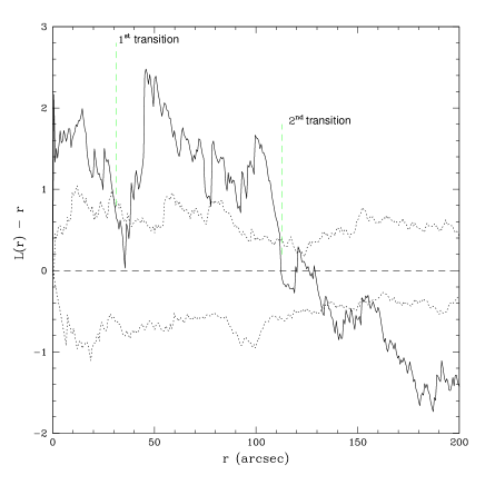
Figure 2: Besag L function for one realization of the Cl 0024+17 galaxy field (solid lines). The Poisson process corresponds to the line L(r)=r (dashed lines). The 95% lower and upper envelopes (averaged over all the MC realizatios of the galaxy field) are presented in dotted lines. Transition scales are marked with vertical green dashed lines

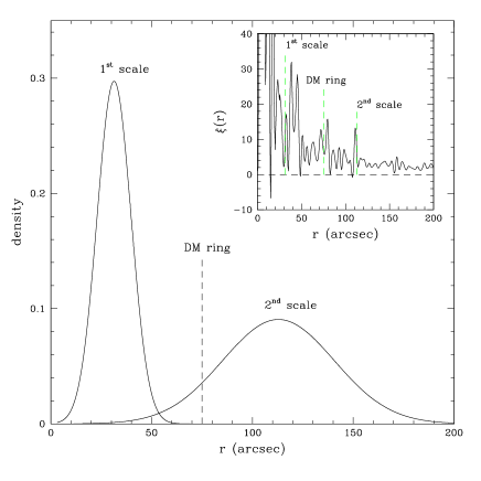
Figure 3: Normal distributions of the $1^{\rm st}$ and $2^{\rm nd}$ transition scales. Vertical dashed lines indicate the position of the DM ring radius. Small box: average correlation function for all MC simulations. DM ring, $1^{\rm st}$ and $2^{\rm nd}$ scales are indicated by green dashed lines.

5 Morphology test

One should be careful not to overinterpret the previous analysis by concluding that the second scale we see in Figure 3 implies that the galaxy distribution around Cl 0024+17 has a luminous counterpart of the dark matter ring. Indeed, this result may have to do with the way observations were done. For instance, the completeness map was constructed after a smoothing procedure using a Gaussian kernel of $30^{\prime\prime}$ [9]. This size is similar to that I have found for the first transition scale, but the separation between the two normal distributions is $\sim$2.7 times this smoothing scale, so it seems that the width of the kernel is not large enough to invalidate the results. On the other hand, the presence of a secondary peak in the distribution about $120^{\prime\prime}$ NW of the cluster center (see Figure 1 and Figure 4 of [9]) can be the responsible for the second scale detected in data. This can be seen in Figure 4, where I plot the perspective view of galaxy distribution also smoothed by a Gaussian kernel of width $30^{\prime\prime}$. Letters A and B indicate the first and second density peaks in the field. Note that the peaks are very close to each other, although clearly distinct. Less distinguishble, however, can be the effect of a spheroidal clump from a ring in the spatial analysis I have applied to data. One way to measure such morphologic effects is now presented.

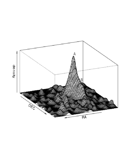
Figure 4: Perspective view of galaxy distribution around Cl 0024+17 smoothed by a Gaussian kernel of width $30^{\prime\prime}$. Letters A and B indicate the the first and second density peaks in the field.

I have built two mock samples made to mimic the cases we want to study. In Model I, we have a central cluster with radius equal to $\mu_{1}=31.4^{\prime\prime}$, plus a clump at $\sim 120^{\prime\prime}$ NW (radius defined as $\mu_{1}/2$) and a Poisson background with same intensity of the Cl 0024+17 field. Both the cluster and the clump have a Hernquist profile (Hernquist 1990), but the cluster is set to have $\sim 4.5$ times the density of the clump (after the Gaussian smoothing). Model II is the central cluster plus a ring at the second scale, $112.9^{\prime\prime}$,with width equal to $\sigma_{2}=21.4^{\prime\prime}$. The density of the cluster is also $\sim 4.5$ times the density of the ring. For each case, 1,000 mock fields were generated. Examples are presented in Figure 5, pannels a and c.

Analysis of these mock fields shows that: (i) in both cases two statistically distinct scales are found – Bartlett and Kruskal-Wallis tests reject the null hypotheses of equal variances and means at $>$99% confidence (see resultant normal distributions in Figure 5, pannels b and d); (ii) however, while in Model II about 94% of the realizations present two scales, this only happens for 61% of the Model I realizations; (iii) the $1^{\rm st}$ Gaussian is narrower for Model I ($\mu_{1}^{\rm I}=30.1,\sigma_{1}^{\rm I}=7.7,\mu_{1}^{\rm II}=31.3,\sigma_{1}^{\rm II}=9.7$) while the $2^{\rm nd}$ Gaussian is narrower for Model II ($\mu_{2}^{\rm I}=117.3,\sigma_{2}^{\rm I}=29.0,\mu_{2}^{\rm II}=120.0,\sigma_{2}^{\rm II}=19.3$); (iv) however, there is no evidence for difference in the results of Models 1 and 2 – Bartlett, ANOVA and Tukey tests indicate only a 0.001% probability of difference between the samples.

The morphology test presented here is quite naive in the sense that neither model reproduces the complexity of the real galaxy field. Exactly for this reason, it may indicate that the methodology presented in Section 3 is not accurate enough to discriminate different morphologies around the galaxy cluster. To improve the results, I have applied a wavelet analysis to the galaxy field of Cl 0024+17. Here I followed the method of [24]. Basically, the coordinates of the galaxies are convolved by a radial Mexican Hat filter on a grid of $N\times N$ pixels. The method leads to a multiscale analysis which starts below the biggest scales, where the whole cluster is detected as a unique structure, and ends with the smallest scale, when approximately only one galaxy lies into the operating area of the wavelet. To obtain the significance level of a given structure I have applied the replica procedure, where many simulations are made by drawing independently $X_{i}$ and $Y_{i}$ from the the $X$ and $Y$ distributions of the sample studied to destroy small-scale correlations, see e.g. [19]. The analysis is then performed on the ”random fields” for the same wavelet scale than the true field. The significance level of a given structure is estimated from the number of images $N_{ext}$ in which maxima greater than the maxima wavelet coefficients are found among the whole set of simulations $N_{set}$. Thus, $P_{SL}=N_{ext}/N_{set}$, see [19]. In Figure 6 we present the isosurfaces of the wavelet coefficients corresponding to the scales $a=64,32,16,~{}{\rm and},8$, respectively (in pixels units for a map of $128\times 128$ pixels). The wavelet scale used is $a=64$ pixels corresponding to 1.0 Mpc. In the top left low resolution image ($a=64$ pixels), we see the prominent central region of the cluster with some density enhament around it, which could suggest an almost symmetric substructure at first sight. However, with increasing resolution, this feature disappears, while at scales $a=32~{}{\rm and}~{}64$ a core + clump structure emerges. Finally, at scale $a=8$ (bottom right image) just a central peak remains. For the two intermediate scales I estimate the significance level of a model core + clump, having found $P_{SL}=0.023$ ($a=32$) and $P_{SL}=0.045$ ($a=16$) (for 1,000 MC simulations), which suggests that such a model cannot be rejected at these scales.

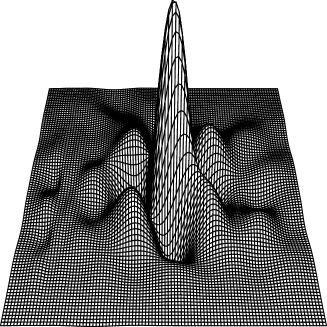
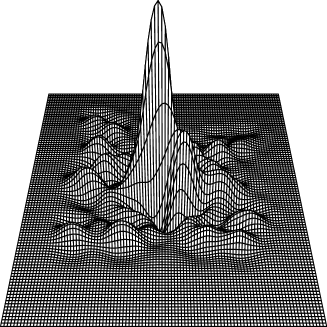
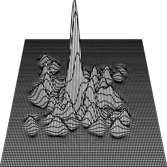
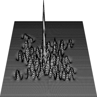
Figure 5: Isosurfaces of the wavelet coefficients in the wavelet analysis on a grid of $128\times 128$ pixels, with $a=64$ pixels corresponding to 1.0 Mpc. The images present decreasing wavelet scales: $a=64,32,16,~{}{\rm and},8$, respectively.

Figure 6: Morphology test. Pannels (a) and (c) exhibit examples of the distribution of points for the cases cluster+clump and cluster+ring, respectively. Pannels (b) and (d) show the result of the spatial analysis: normal distributions related to the scales detected for both geometries.

6 Anisotropy test

Spheroidal clumps and rings (and possibly other shapes) may produce approximately the same results after spatial analysis. However, in the case of comparing rings and clumps, there is a remaining property to be tested: the anisotropy of the signal around the cluster. This second test is now introduced.

For the projected distribution, anisotropy can be probed by the reduced second-order moment measure ${\mathcal{K}}$ of a point pattern (e.g. Illian et al. 2008 and references therein). In this work, we estimate ${\mathcal{K}}$ with using the library spatstat under R statistical package. The routine Kmeasure executes the following steps:

1. it takes a point pattern,

2. and forms the list of all pairs of distinct points in the pattern,

3. then computes the vectors that join the first point to the second point in each pair,

4. and treats these vectors as a pattern of ‘points’,

5. finally applyies a Gaussian kernel smoother to them (keeping the kernel width $30^{\prime\prime}$, see Sections 4 and 5).

The algorithm approximates the point pattern and its window by a binary pixel image, introduces a Gaussian smoothing kernel and uses the Fast Fourier Transform to make a density estimate $\kappa$. The density estimate of $\kappa$ is returned in the form of a real-valued pixel image. The $\hat{\mathcal{K}}$ estimator is defined as the the expected number of points lying within a distance $r_{max}$ of a typical point, and with displacement vector having an orientation in the range $[\alpha,\beta]$. This can be computed by summing the entries over the relevant region, i.e, the sector of the disc of radius $x$ centred at the origin with angular range $[\alpha,\beta]$. Hence, we can compute a measure of anisotropy, A, as integrals of the form

$$A\equiv\int_{0}^{r_{max}}\int_{\alpha}^{\beta}d\kappa(r,\theta).$$ (7)

Recall that Ripley function (both in first and second order) is used to test the hypothesis that a given planar point pattern is a realization of a Poisson process. In the case of vectors instead of points, the second-order orientation analysis can be done around the center of the field. A nearly flat anisotropy profile would be consistent with a Poisson process $A\approx 0$. Thus, the idea here is to look for significant anisotropies in integral (7) for angular steps ${\rm\Delta\theta=\beta-\alpha}$. The choice of ${\rm\Delta\theta}$ is arbitrary, and it was set to be ${\rm\Delta\theta}=15^{\circ}$, based in the following analysis. We take 1,000 realizations of a controlled sample corresponding to a point pattern given by a Poisson distribution plus a Hernquist spheroid (Hernquist 1990) located at $\sim 100^{\prime\prime}$ and making an angle of $45^{\circ}$ around the center. To justify our choice of $\Delta\theta$ we present in Figure 7 the analyses for the case for $\Delta\theta=5^{\circ},15^{\circ},~{}{\rm and}~{}30^{\circ}$. For $\Delta\theta=5^{\circ}$, we still detect the peak, but now there are secondary peaks and a more noisy behaviour for $\langle A\rangle$. For $\Delta\theta=30^{\circ}$, the peak is still there, but now it is less significant. This result suggests that in the limit of too small $\Delta\theta$ we have a noisy anisotropy curve (possibly with false peaks), while in the limit of very large $\Delta\theta$ the signal can be completely lost. Actually, in the approximate range $[12^{\circ},18^{\circ}]$ the resultant anisotropy profiles are almost indistinguishable, with relative differences $\lesssim 3\%$.

Figure 7: Anisotropy profiles of a controlled sample (Poisson + clump at $45^{\circ}$). Solid lines for $\Delta\theta=15^{\circ}$; dotted lines for $\Delta\theta=5^{\circ}$; and dashed lines for $\Delta\theta=30^{\circ}$.

Results of the anisotropy test for the averaged samples are presented in Figure 8. Note that Model I (although very simplified) reproduces fairly well the anisotropy profile of real data, exhibiting a peak around $110^{\circ}$ (or the supplementary angle $290^{\circ}$), a direction corresponding to the axis crossing the NW quadrant. On the contrary, Model II has a flatter anisotropy profile. In fact, Kolmogorov-Smirnov test is consistent with the null hypothesis that Data and Model I samples come from the same distribution. This is not true for the KS test comparing Data and Model II samples, and Model I and Model II samples (see p-values in Figure 8). I also have applied a Welch two-sample t-test to find if the anisotropy profiles are stochastically higher between each other. Again, the results indicate that both Data and Model I have profiles significantly higher than that of Model II. Also, there is not a significant difference between Data and Model I profiles (see p-values in Figure 8). This all means that the galaxy field around Cl 0024+17 is more consistent with an anisotropic cluster+clump distribution instead of a cluster+ring one.

Morphology and anisotropy tests are not totally conclusive, but they suggest that the second scale found in data is more probable to be associated to the clump at $\sim 120^{\prime\prime}$ NW from the cluster center than to a ring of galaxies, although this feature cannot be discarded by spatial analysis alone.

Figure 8: Anisotropy test. The anisotropy profiles for the averaged samples are presented as follows: Data – solid lines; Model I – dotted lines; Model II – dashed lines. p-values associated to KS test and Welch t-test are presented in the upper left corner table.

7 Summary and Discussion

By considering the planar galaxy distribution around Cl 0024+17 as a SPP, I have applied some tools of spatial statistics analysis to probe the existence of an extended structured in this cluster. The catalog was corrected through 1,000 MC realizations of original the sample, following the completeness map of [8]. Based on the Besag L-function curves I have identified two distinct physical scales where the null hypothesis that the data came of a Poisson process is rejected at 95% confidence. Values found for the two scales present normal distributions: $\mu_{1}=31.4^{\prime\prime};\sigma_{1}=8.4^{\prime\prime}$ and $\mu_{1}=112.9^{\prime\prime};\sigma_{2}=21.4^{\prime\prime}$. Both Bartlett and Kruskal-Wallis statistical tests indicate these normals are significantly unequal both in variances and means. This reinforces the idea of two density peaks in the Cl 0024+17 field. Also, the analysis of the averaged correlation function for all MC realizations suggests that at $\sim 50^{\prime\prime}$ may be the maximum scale for the core of the system. This scale is approximately at the intersection of the normal distributions found for the two transition scales. The DM ring radius and the $2^{\rm nd}$ transition scale are approximately coincidents with the highest peaks of $\xi(r)$ after $\sim 50^{\prime\prime}$. However, morphology and anisotropy tests based on simulations of 1,000 mock fields for cluster+clump and cluster+ring models are not conclusive about interpreting the second scale as a ring of galaxies. However, a wavelet analysis of the field points out that a cluster+clump model cannot be rejected at scales $a=32$ pixels (0.50 Mpc) and $a=16$ pixels (0.25 Mpc). Finally, the anisotropy test also suggests that the second scale found in data is more probable to be associated to the clump at $\sim 120^{\prime\prime}$ NW from the cluster center than to a ring of galaxies.

Summing up this work, the analyses presented in Sections 4, 5 and 6 are not indicative that galaxies follow dark matter around Cl 0024+17, but the methodology based on spatial patterns examination seems to have good sensitivity to find physical scales in galaxy systems (both in radial and angular coordinates). It could turn a useful tool to study galaxy (and maybe other astrophysical) systems in general. Spatial analysis (followed by subsidiary morphology and anisotropy tests) could be a poweful technique to probe remnant substructures of clusters collisions using galaxy data alone. Analysing a large dataset of galaxy clusters, we could identify candidates to bullet-type clusters by the presence of at least two transition scales. Also, the approach can introduce a new estimator for galaxy systems radii based only on the scales detected in data [22]. Finally, this method can be directly applied to data from N-body simulations of cluster collisions. Some sensitivity to initial conditions could be tested not only looking for bumps in the density projected along the collision axis, but also with the dark matter particles interaction range. This is an interesting test to be done, since a recent study suggests that the ring-like feature of Cl 0024+17 (and similar cases) would be associated to very improbable initial velocity distributions [27].

8 Acknowledgments

I thank the referee for very useful suggestions. I am grateful to A.C. Schilling and B. Carvalho for helpful statistical discussions. I also thank the support of CNPq, under grant 201322/2007-2. Finally, I thank the Fermilab for the hospitality.

References

- Baddeley [2008] Baddeley, A., Analysing spatial point patterns in R, Workshop Notes (2008)
- Baddeley et al. [2000] Baddeley, A., Moller, J. and Waagepetersen, R. 2000, Statistica Neerlandica, 54, 329
- Baddeley & Turner [2006] Baddeley, A. & Turner, R. 2006, in Case Studies in Spatial Point Process Modeling, Lecture Notes in Statistics 185, Springer-Verlag, New York, pp. 23-76
- Besag [1977] Besag, J.E. 1977, J. Roy. Statist. Soc. B, 39, 193
- Broadhurst et al. [2000] Broadhurst, T., Huang, X., Frye, B. & Ellis, R. 2000 ApJ, 534 L15
- Clowe et al. [2006] Clowe, D., Bradac, M., Gonzalez, A.H., Markevitch, A.V., Randall, S.W., Jones, C. & Zaritsky 2006, ApJ Letters, 648, L109
- Comerford et al. [2006] Comerford, J.M., Meneghetti, M., Bartelmann, M. & Schirmer, M. 2006, ApJ, 642, 39
- Czoske et al. [2001] Czoske, O., Kneib, J.-P., Soucail, G., Bridges, T.J., Mellier, Y. & Cuillandre, J.-C. 2001, A& A, 372 391
- Czoske et al. [2002] Czoske, O., Moore, B., Kneib, J.-P. & Sucail, G. 2002, A& A, 386, 31
- Davis et al. [1985] Davis,M., Efstathiou, G., Frenk, C., & White, S.D.M. 1985, ApJ, 292, 371
- Hernquist [1990] Hernquist, L. 1990, ApJ, 356, 359
- Humason& Sandage [1957] Humason, M.L. & Sandage, A. 1957, in Carnegie Yearbook 1956 (Washington, DC: Carnegie Inst. Washington), 61
- see e.g. Illian et al. [2008] Illian, J., Penttinen, A., Stoyan, H. & Stoyan, D. 2008, Statistical Analysis and Modelling of Spatial Point Patterns, Ed. John Wiley & Sons Ltd
- Jee et al. [2005a] Jee, M.J., White, R.L., Benitez, N., Ford, H.C., Blakeslee, J.P., Rosati, P., Demarco, R. & Illingworth, G.D. 2005a, ApJ, 618, 46
- Jee et al. [2005b] Jee, M.J., White, R.L., Ford, H.C., Blakeslee, J.P., Illingworth, G.D., Coe, D.A. & Tran, K.V.H. 2005b, ApJ, 634, 813
- Jee et al. [2007] Jee, M.J et al. 2007, ApJ, 661, 728
- Markevitch et. al. [2002] Markevitch, M., Gonzalez, A.H., David, L., Vikhlinin, A., Murray, S., Forman, W., Jones, C. & Tucker, W. 2002, ApJ, 567, L27
- Markevitch [2007] Markevitch, M. 2007, Phys. Rep. 443, 1
- Escalera & Mazure [1992] Escalera, E. & Mazure, A. 1992, ApJ, 388, 23
- Ota et al. [2004] Ota, N., Pointecouteau, E., Hattori, M. & Mitsuda, K. 2004, ApJ, 601 120
- Qin, Shan & Tilquin [2008] Qin, B., Shan, H.-Y. & Tilquin, A. 2008, ApJ 679, L81
- Ribeiro & Lopes [2009] Ribeiro, A.L.B. & Lopes, P.A.A. 2009, in preparation
- Ripley [1977] Ripley, B.D. 1977, J. Roy. Statist. Soc. B, 41, 368
- Slezak et al. [1990] Slezak, E., Bijaoui, A. and Mars, G. 1990, A& A, 227, 301
- Tyson et al. [1998] Tyson, J.A., Kochanski, G.P. & dell’Antonio, I.P. 1998, ApJ, 498, L107
- Zhang et al. [2005] Zhang, Y.-Y., Böhringer, H., Meiller, Y., Soucail, G. & Forman, W. 2005, A& A, 429, 85
- ZuHone, Lamb & Ricker [2008] ZuHone, J.A., Lamb, D.Q. & Ricker, P.M. 2008, astro-ph/0809.3252