A model for the orientational ordering of the plant microtubule cortical array

Abstract

The plant microtubule cortical array is a striking feature of all growing plant cells. It consists of a more or less homogeneously distributed array of highly aligned microtubules connected to the inner side of the plasma membrane and oriented transversely to the cell growth axis. Here we formulate a continuum model to describe the origin of orientational order in such confined arrays of dynamical microtubules. The model is based on recent experimental observations that show that a growing cortical microtubule can interact through angle dependent collisions with pre-existing microtubules that can lead either to co-alignment of the growth, retraction through catastrophe induction or crossing over the encountered microtubule. We identify a single control parameter, which is fully determined by the nucleation rate and intrinsic dynamics of individual microtubules. We solve the model analytically in the stationary isotropic phase, discuss the limits of stability of this isotropic phase, and explicitly solve for the ordered stationary states in a simplified version of the model.

I Introduction

Most plant cells grow by uniaxial expansion. Establishing and maintaining this characteristic anisotropic growth mode requires regulatory mechanisms that are robust, and, in addition, sensitive to the cell geometry. A major role in this process is played by microtubules, highly dynamic filamentous protein aggregates that form one of the components of the cytoskeleton of all eukaryotic organisms (see Ref. [1], chapter 16). In growing plant cells microtubules are confined to a thin layer of cytoplasm just inside the cell plasma membrane. Here they form the so-called cortical array, an ordered structure formed by highly aligned (bundles of) microtubules oriented transversely to the growth direction [2]. This structure is unique to plant cells and there is evidence that it controls the direction of cell expansion by guiding the mobile transmembrane protein complexes that deposit long cellulose microfibrils in the plant cell wall [3]. These cellulose microfibrils are the main structural elements of the cell wall, which, for mechanical reasons, are also transversely oriented to the cell axis in growing cells [4]. An in vivo image of the array and a schematic are shown in Figure 1.

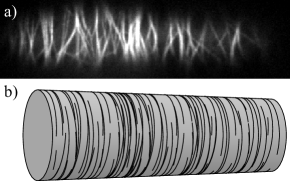
Figure 1: (a) Fluorescently labelled microtubules in a Tobacco BY-2 cell expressing GFP:TUA6. Image courtesy of Jelmer Lindeboom, Wageningen University. (b) Schematic representation of a plant cell cortical array.

In vivo imaging of microtubules labelled with fluorescent proteins in plant cells by several groups has shown how the cortical array is established both following cell division and after microtubule depolymerizing drug (oryzalin) treatment [5, 6, 7, 8, 3, 2]. In these studies microtubules are seen to nucleate at the cortex and then develop from an initially disorganized state into the transverse ordered array over a time period on the order of one hour. The nature of the self-organization process by which the specific spatial and orientational patterning of this cytoskeletal structure is achieved is as yet only partially understood and forms the subject of this work.

An important aspect of the problem is the nature of localization of the microtubules to the cortical region. Fluorescence recovery after photo-bleaching (FRAP) experiments by Shaw et al. [7] showed that the microtubules are fixed in space, so any apparent mobility of microtubules is due to ‘treadmilling’, the process of simultaneous polymerization at one end and depolymerization at the other end. So, cortical microtubules do not translate or rotate as a whole. The same authors also did not detect detachment or (re)attachment of microtubules to the cell cortex, apart from some growing ends of single microtubules moving out of focus and found no evidence for motors working in the cortical array. These experiments indicate that the microtubules in the cortical array are fixed to the inside of the cell membrane. Electron microscopy has also shown cross-bridges between cortical microtubules and the membrane [9]. It is therefore widely assumed that there are linker proteins that anchor the microtubules through the plasma membrane to the rigid cell wall, although their molecular identity is under debate [10, 11, 12, 13, 14]. Since the cortical microtubules are effectively confined to a 2D surface, they can interact through ‘collisions’ that occur when the polymerizing tip of a growing microtubule encounters a pre-existing microtubule. The resulting dynamical interaction events were first characterized by Dixit and Cyr [15] in tobacco Bright Yellow-2 (BY-2) cells. They observed three different possible outcomes: (i) zippering: a growing microtubule bending towards the direction of the microtubule encountered, which occurs only when the angle of incidence is relatively small ($\lesssim 40^{\circ}$) (ii) induced catastrophe: an initially growing microtubule switching to a shrinking state and retracting after the collision, an effect predominant at larger angles of incidence and (iii) cross-over: a growing microtubule ‘slipping over’ the one encountered and continuing to grow in its original direction.

There are clearly many coupled mechanisms at work in this complex biological system contributing to the assembly and maintenance of this microtubule cortical array structure. We are interested in understanding what are the main contributing factors and how their interplay leads to the observed orientational ordering. With this aim we develop a coarse-grained model, incorporating all the effects discussed above. Our emphasis on the plant-specific biological mechanism of the ordering in the cortical array distinguishes our approach from earlier work.

Over the years, various models for self-organization of cytoskeletal filaments (and polar rods in general) have been proposed [16, 17, 18, 19], and the model by Zumdieck et al. [20] was applied to the plant cortex. However, in each of these models the filaments are assumed to have rotational and, in most cases, translational degrees of freedom. This is inconsistent with the fact that the plant cortical microtubules are stably anchored. Inspired by the experimental results of Dixit and Cyr [15], Baulin et al. [21] were the first to report on a two dimensional dynamical system of treadmilling and colliding microtubules. Their focus was on establishing the minimal interactions needed to generate dynamical alignment. Using stochastic simulations they showed that a pausing mechanism, whereby a growing microtubule stalls against another microtubule until the latter moves away, can indeed lead to ordering. Stalling, however, is not often observed in the cortical array. Moreover their model lacks dynamic instabilities, i.e. catastrophes, both spontaneous and induced, and rescues, and employs a form of deterministic microtubule motion, which is arguably unrealistic in view of the observed dynamics.

The outline of the paper is as follows. In section II we formulate our course-grained model starting from a description of the dynamics of individual microtubules. We then construct the continuity equations that couple the densities of growing, shrinking and inactive microtubule segments due to the intrinsic and collisional dynamics. In the steady state we can reduce the initial set of equations to four coupled non-linear integral equations. We then perform a dimensional analysis to identify the relevant control parameter of the system. In section III we present the results of our model. We first solve the model analytically in the isotropic stationary state. Using a bifurcation analysis we then determine the critical values of the control parameter at which the system develops ordered solutions. We interpret these results in terms of the physical parameters of microtubule segment length and mesh size. Finally, we formulate a minimal model with realistic interaction parameters that we can solve numerically to obtain all stationary ordered solutions. We close by giving arguments for the stability of these solutions. The paper concludes with a discussion section. An appendix outlines further details of the numerical solution technique employed.

II Model

II.1 Description of the microtubules and their dynamics

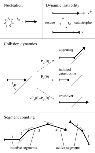
Figure 2: Schematic representation of the model interaction. The microtubule of interest is drawn in black and other microtubules that it encounters are in grey. The active segments of the black microtubule have an arrow head indicating growth or shrinkage whereas inactive segments end in the junction with the following segment depicted by a dot. See also the description of the parameters in table 1.

As described in the introduction we confine the configuration of the microtubules to a 2D plane. Since collision-induced zippering events can cause microtubules to bend along the direction of preexisting ones, we divide each microtubule into distinct segments with a fixed orientation. We treat these segments as straight rigid rods. This is justifiable since the persistence length $l_{p}$ of microtubules is long ($\sim\mathrm{mm}$) compared to the average length of a microtubule ($\sim 10\mu\mathrm{m}$) and, as mentioned above, adhesion to the plasma membrane further inhibits thermal motion.

Microtubules are known to be dynamic in that they are continually growing or shrinking by (de)polymerization. We use the standard two-state dynamic instability model of Dogterom and Leibler [22] which assumes that each microtubule has a ‘plus’ end, located on the final segment of each microtubule, that is either growing (labelled by $+$) with speed $v^{+}$ or shrinking (labelled by $-$) with speed $v^{-}$. This plus end can switch stochastically from growing to shrinking (a so-called ‘catastrophe’) with rate $r_{\textrm{c}}$, or from shrinking to growing (a so-called ‘rescue’) with rate $r_{\textrm{r}}$ in a process known as dynamic instability.

We model the creation of new microtubules with a constant, homogeneous, isotropic nucleation rate $r_{\textrm{n}}$ in the plane of the 2D model. In vivo nucleation appears to occur at the cortex and has been observed to occur in random orientations unattached to pre-existing microtubules [7]. Although microtubules have also been observed to nucleate from by $\gamma$-tubulin complexes binding to pre-existing microtubules [23, 24, 2] we ignore this possibility for simplicity’s sake. By the same token we disregard the possibility of the shrinking of microtubules at their less active ‘minus’ end, leading to motion through the ‘treadmilling’ mechanism [25]. The initial segment of each microtubule therefore remains attached to the nucleation point in our model.

We call the final segment of a microtubule, which contains the growing or shrinking tip, active and all the remaining ones, which do not change their length, inactive (labelled by $0$). A cartoon of an an individual microtubule according to these definitions is depicted in figure 2. When a microtubule collides with another microtubule and experiences a zippering event, its active segment is converted into an inactive segment, and a new active segment is created alongside the encountered microtubule. The inverse can also occur: if the active segment shrinks to zero length, a previously inactive segment in another direction can be reactivated. An induced catastrophe event simply causes the growing active segment to become a shrinking one, as is the case for spontaneous catastrophes. Finally, a crossover results in the growing active segment continuing to grow unperturbed.

In figure 3 we present the relative probabilities for zippering, induced catastrophes and crossovers as a result of collisions between microtubules, based on the data provided by Dixit and Cyr [15]. We assume that there are no microtubule polarity effects, as they were not reported. The probabilities $P_{\textrm{z}}(\theta-\theta^{\prime})$, $P_{\textrm{x}}(\theta-\theta^{\prime})$ and $P_{\textrm{c}}(\theta-\theta^{\prime})$ for zippering, cross-overs and induced catastrophes respectively are therefore even functions of the angle difference $\theta-\theta^{\prime}$ defined by their values on the interval $[0,\frac{\pi}{2}]$. In this article we will use only the following minimal set of properties, which are qualitatively supported by the data. Firstly, zippering becomes less likely for increasing angle of incidence, and is effectively zero at $\theta-\theta^{\prime}=\frac{\pi}{2}$, which is reasonable as the energy associated with bending the microtubule increases with angle. Secondly, the probability for induced catastrophes monotonically increases with increasing angle of incidence, reaching a maximum at $\theta-\theta^{\prime}=\frac{\pi}{2}$, consistent with observations that indicate that a microtubule which is hindered in its growth will undergo a catastrophe at a rate that depends inversely on its growth speed [26].

Figure 3: Probabilities for zippering, cross-overs and catastrophes as deduced from the observations of [15] (combined data from MBD-DsRed and YFP-TUA6 labelling). Light grey shaded region: fraction of zippering events. Dark grey shaded region: fraction of induced catastrophes. White region: fraction of crossovers. Every data point is located at the centre of the corresponding bin, and the shaded regions have been extended to the boundaries using horizontal lines. The corresponding lowest order Fourier coefficients of the interaction functions are: $\hat{c}_{0}=0.59$, $\hat{c}_{2}=-0.36$, $\hat{z}_{0}=0.24$ (computed using numerical integration of the product of $\left|\sin{\theta}\right|$ and a piecewise linear interpolation of the data).

II.2 Continuum model

Table 1: Overview of all parameters and variables in natural dimensions

Parameters	Description	Dimensions
$v^{+}$	growth speed	$\left[\text{length}\right]/\left[\text{time}\right]$
$v^{-}$	shrinkage speed	$\left[\text{length}\right]/\left[\text{time}\right]$
$r_{\textrm{c}}$	catastrophe rate	$1/\left[\text{time}\right]$
$r_{\textrm{r}}$	rescue rate	$1/\left[\text{time}\right]$
$r_{\textrm{n}}$	nucleation rate	$\left[\text{length}\right]^{-2}\left[\text{time}\right]^{-1}$
$P_{\textrm{c}}(\theta)$	probability of induced catastrophe upon collision	1
$P_{\textrm{z}}(\theta)$	probability of zippering upon collision	1
Synthetic parameters
$g=\frac{r_{\textrm{r}}}{v^{-}}-\frac{r_{\textrm{c}}}{v^{+}}$	growth parameter	$1/\left[\text{time}\right]$
$u=1+\frac{v^{+}}{v^{-}}$	speed ratio	1
$c(\theta)=\mathrm{sin}(|\theta|)P_{\textrm{c}}(\theta)\longleftrightarrow\left\{\hat{c}_{n}\right\}$	effective catastrophic collision probability	1
$z(\theta)=\mathrm{sin}(|\theta|)P_{\textrm{z}}(\theta)\longleftrightarrow\left\{\hat{z}_{n}\right\}$	effective zippering probability	1
Dependent variables
$k\left(\theta\right)$	microtubule length density	$\left[\text{length}\right]^{-1}\left[\text{radian}\right]^{-1}$
$l\left(\theta\right)$	average microtubule segment length	$\left[\text{length}\right]$
$\left\{m_{i}^{+}\left(l,\theta\right),m_{i}^{-}\left(l,\theta\right),m_{i}^{0}\left(l,\theta\right)\right\}$	density of growing/shrinking/inactive segments
	with length $l$ and direction $\theta$	$\left[\text{length}\right]^{-3}\left[\text{radian}\right]^{-1}$

Since there are many ($\approx 10^{2}$ - $10^{3}$) microtubules, each of which can have multiple segments, in the cortical array of a typical interphase plant cell we treat the system using a coarse-grained description. In this approach, instead of individual microtubules, we consider local densities of microtubule segments. This approximation is reasonable as long as the length scale of an individual microtubule segment is small compared to the linear dimensions of the cell. From the outset we assume that the system is (and remains) spatially homogeneous, and we will eventually restrict ourselves to the steady-state solutions. In order to deal with the memory effect caused by the isotropic nucleation, followed by subsequent reorienting zippering events, we need to keep track of the segment number $i$, which starts at $1$ for the segments connected to their nucleation site and increases by unity at each zippering event. Our fundamental variables are therefore the areal number densities $m_{i}^{\sigma}(l,\theta,t)$ of segments in state $\sigma\in\left\{0,-,+\right\}$ with segment number $i$ having length $l$ and orientation $\theta$ (measured from an arbitrary axis) at time $t.$ These densities obey a set of master equations that can symbolically be written as

$$\partial_{t}m_{i}^{+}(l_{i},\theta_{i},t) =\Phi_{\text{{growth}}}+\Phi_{\text{{rescue}}}-\Phi_{\text{{spont. cat.}}}$$

$$-\Phi_{\text{{induced cat.}}}-\Phi_{\text{{zipper}}}$$ (1a)

$$\partial_{t}m_{i}^{-}(l_{i},\theta_{i},t) =\Phi_{\text{{shrinkage}}}-\Phi_{\text{{rescue}}}+\Phi_{\text{{spont. cat.}}}$$

$$+\Phi_{\text{{induced cat.}}}+\Phi_{\text{{reactivation}}}$$ (1b)

$$\partial_{t}m_{i}^{0}(l_{i},\theta_{i},t) =+\Phi_{\text{{zipper}}}-\Phi_{\text{{reactivation}}}$$ (1c)

The flux terms $\Phi_{\text{{event}}}$ couple the equations for the growing, shrinking and inactive segments and between different values of $i$. Equations (1) must be supplemented by a set of boundary conditions for the growing segments at $l=0$. For the initial segment ($i=1$) this reflects the isotropic nucleation of new microtubules, given by

$$v^{+}m_{1}^{+}(l_{1}=0,\theta,t)=\frac{r_{\textrm{n}}}{2\pi},$$ (2)

where $r_{\textrm{n}}$ is nucleation rate. For the subsequent segments $i>1$, this ‘nucleation’ of growing segments is the result of the zippering of segments with index $i-1$. Defining $\varphi_{\text{zipper}}\left(\theta_{i-1}\rightarrow\theta_{i},l_{i-1},t\right)$ as the flux of $i$-segments with angle $\theta_{i}$ and length $l_{i}$ zippering into angle $\theta_{i+1}$ at time $t$ (this will be made explicit in equation (13)), we obtain the boundary condition

$$v^{+}m_{i\geq 2}^{+}(l_{i}=0,\theta_{i},t) =$$

$$\int\mathrm{d}l_{i-1}\int\mathrm{d}\theta_{i-1} \;\varphi_{\text{zipper}}\left(\theta_{i-1}\rightarrow\theta_{i},l_{i-1},t\right)\;.$$ (3)

Generally, this leads to a qualitatively different boundary condition for every value of $i$. The model therefore consists of an infinite set of coupled equations, three for every value of $i$. However, in section II.3 we will show that in the steady state, this can be reduced to a finite set by summing over all segment indices $i$. In the following, we derive explicit expressions for each of the flux terms $\Phi_{\text{{event}}}$.

II.2.1 Growth and shrinkage terms: $\Phi_{\text{growth}}$, $\Phi_{\text{shrinkage}}$

$\Phi_{\text{{growth}}}$ in Equation (1a) corresponds to the length increase of the growing segments. For segment growth in isolation, the length increase in a small time interval $\delta t$ is given by $v^{+}\delta t,$ where $v^{+}$ is the growth velocity, and we have $m^{+}(l+v^{+}\delta t,\theta,t+\delta t)=m^{+}(l,\theta,t)$. By expanding the left hand term to first order in $\delta t,$ we find

$$\partial_{t}m_{i}^{+}(l,\theta,t)=-v^{+}\partial_{l}m_{i}^{+}(l,\theta,t)\equiv\Phi_{\text{{growth}}}$$ (4)

A similar derivation yields that

$$\partial_{t}m_{i}^{-}(l,\theta,t)=v^{-}\partial_{l}m_{i}^{-}(l,\theta,t)\equiv\Phi_{\text{{shrink}}}$$ (5)

where $v^{-}$ is the shrinking velocity.

II.2.2 Dynamic instability terms: $\Phi_{\text{rescue}}$ ,$\Phi_{\text{spont. cat.}}$

$\Phi_{\text{{rescue}}}$ and $\Phi_{\text{{spont. cat.}}}$ in equations (1a) and (1b) correspond to the fluxes due to the spontaneous rescues and spontaneous catastrophe respectively and are simply given by

$$\Phi_{\text{{rescue}}}= r_{\textrm{r}}m_{i}^{-}(l_{i},\theta_{i},t)$$ (6)

$$\Phi_{\text{{spont. cat.}}}= r_{\textrm{c}}m_{i}^{+}(l_{i},\theta_{i},t)$$ (7)

where $r_{\textrm{r}}$ is the spontaneous rescue rate and $r_{\textrm{c}}$ is the spontaneous catastrophe rate.

So far, we have described the first three terms of equations (1a) and (1b) (growth, shrinkage and dynamic instability terms). Together, these fully describe a system of non-interacting microtubules, in which also the boundary condition (3) vanishes due to the absence of zippering. In this special case we recover the well-known equations introduced by Dogterom and Leibler [22] (for $i=1$).

II.2.3 Interaction terms: $\Phi_{\text{induced cat.}}$, $\Phi_{\text{zipper}}$

An interaction can occur when a growing active microtubule segment collides with another segment, irrespective of the latter’s state and length. This prompts the definition of the total length density $k(\theta,t)$ of all microtubule segments in direction $\theta$ at time $t$, given by:

$$k(\theta,t)=\sum_{i}\int\mathrm{d}l_{i}\,l_{i}(m_{i}^{+}(l_{i},\theta,t)+m_{i}^{-}(l_{i},\theta,t)+m_{i}^{0}(l_{i},\theta,t))\;$$ (8)

The density of collisions of a microtubule segment growing in direction $\theta$ with other segments in direction $\theta^{\prime}$ is determined by the geometrical projection

$$\left|\mathrm{sin}(\theta-\theta^{\prime})\right|k(\theta^{\prime},t),$$ (9)

where the presence of the $\mathrm{sin}(\theta-\theta^{\prime})$ factor ensures the correct geometrical weighting reflecting the fact that parallel segments do not collide. When a collision occurs, one of the three possible events, induced catastrophe $\left(c\right),$ zippering $\left(z\right)$ or cross-over $\left(x\right)$ occurs, with probabilities $P_{\textrm{c}}\left(\theta-\theta^{\prime}\right),$ $P_{\textrm{z}}\left(\theta-\theta^{\prime}\right)$ and $P_{\textrm{x}}\left(\theta-\theta^{\prime}\right)$ respectively. These probabilities can (and in-vivo do, see Figure 3) depend on the relative angle $\theta-\theta^{\prime}$ between the incoming segment and the  ‘scatterer’. For convenience sake we absorb the geometrical factor $\left|\mathrm{sin}(\theta-\theta^{\prime})\right|$ into the probabilities, by defining $f\left(\theta-\theta^{\prime}\right)=\left|\mathrm{sin}(\theta-\theta^{\prime})\right|P_{f}\left(\theta-\theta^{\prime}\right)$ for all events $f\in\left\{c,z,x\right\}.$ The incoming flux of growing microtubule segments with given segment number, length and orientation is given by $v^{+}m_{i}^{+}(l,\theta,t).$ With these definitions we can write the interaction terms as

$$\Phi_{\text{induced cat.}} =v^{+}m_{i}^{+}(l_{i},\theta_{i},t)\int\mathrm{d}\theta^{\prime}\,c(\theta_{i}-\theta^{\prime})k(\theta^{\prime},t)\;$$ (10)

$$\Phi_{\text{zipper}} =v^{+}m_{i}^{+}(l_{i},\theta_{i},t)\int\mathrm{d}\theta^{\prime}\,z(\theta_{i}-\theta^{\prime})k(\theta^{\prime},t)\;$$ (11)

The analogous term for crossovers is not used, because the occurrence of a crossover event has no effect on the growth of a microtubule.

II.2.4 Reactivation term: $\Phi_{\text{reactivation}}$

The reactivation term $\Phi_{\text{reactivation}}$ corresponds to the flux of active microtubule segments, with segment number $i+1,$ that, by shrinking to length zero, reactivate a previously inactive segment, effectively undoing a past zippering event and so create a new, shrinking, active segment with segment number $i.$ The incoming flux of of such segments coming from a given direction $\theta_{i+1}$ is given by $v^{-}m_{i+1}^{-}(l_{i+1}=0,\theta_{i+1},t)$. The reactivation flux is given by

$$\Phi_{\text{reactivation}}=\\ \int d\theta_{i+1}\,v^{-}m_{i+1}^{-}(l_{i+1}=0,\theta_{i+1},t)p_{\text{unzip}}(\theta_{i},l_{i}|\theta_{i+1},t),$$ (12)

where the ‘unzippering’ distribution $p_{\text{unzip}}(\theta_{i},l_{i}|\theta_{i+1},t)$ gives the probability that the shrinking microtubule reactivates an inactive segment with orientation $\theta_{i}$ and length $l_{i}$. This distribution will be determined below.

A microtubule that has zippered will take a certain amount of time $\tau$ to undergo a catastrophe and return to the zippering location, where $\tau$ is a stochastic variable. The unzipppering flux from direction $\theta_{i+1}$ at time $t$ consists of microtubules that had zippered at a range of times $t-\tau$ and have now returned to the zippering location. This implicitly defines an originating time distribution $p_{\text{origin}}\left(t-\tau|\theta_{i+1},t\right)$ for the returning microtubules. Furthermore, because the evolution of a microtubule between the zippering event and its return to the same location does not depend on the previous segments, the segment that is re-activated by a microtubule returning to the zippering position after a time $\tau$ should be selected proportional to the ‘forward’ zippering flux at time $t-\tau$. The forward flux $\varphi_{\text{zipper}}\left(\theta_{i}\rightarrow\theta_{i+1},l_{i},t\right)$ of microtubules with length $l_{i}$ and angle $\theta_{i}$ zippering into angle $\theta_{i+1}$ is defined in accordance with equation (11) as

$$\varphi_{\text{zipper}}\left(\theta_{i}\rightarrow\theta_{i+1},l_{i},t\right)=\\ v^{+}m_{i}^{+}(l_{i},\theta_{i},t)z(\theta_{i}-\theta_{i+1})k(\theta_{i+1},t).$$ (13)

At each of the originating times $t-\tau$, the distribution of microtubules that zipper into the direction $\theta_{i+1}$ with length $l_{i}$ and orientation $\theta_{i}$ is given by

$$p_{\text{zip}}(\theta_{i},l_{i}|\theta_{i+1},t-\tau)=\frac{\varphi_{\text{zipper}}\left(\theta_{i}\rightarrow\theta_{i+1},l_{i},t-\tau\right)}{\int\mathrm{d}l^{\prime}\mathrm{d}\theta^{\prime}\;\varphi_{\text{zipper}}(\theta^{\prime}\rightarrow\theta_{i+1},l^{\prime},t-\tau)\;}.$$ (14)

The probability distributions $p_{\text{origin}}\left(t-\tau|\theta_{i+1},t\right)$ and $p_{\text{zip}}(\theta_{i},l_{i}|\theta_{i+1},t-\tau)$ can be combined to determine the unzippering distribution

$$p_{\text{unzip}}(\theta_{i},l_{i}|\theta_{i+1},t)=\int_{0}^{t}\!\mathrm{d}\tau\,p_{\text{origin}}\left(t-\tau|\theta_{i+1},t\right)\times\\ \frac{\varphi_{\text{zipper}}\left(\theta_{i}\rightarrow\theta_{i+1},l_{i},t-\tau\right)}{\int\mathrm{d}l^{\prime}\mathrm{d}\theta^{\prime}\;\varphi_{\text{zipper}}(\theta^{\prime}\rightarrow\theta_{i+1},l^{\prime},t-\tau)\;},$$ (15)

where we assume the system evolved from an initial condition at $t_{0}=0$ in which no microtubules were present. Clearly all the complicated history dependence of the system is hidden in the originating time distribution. However, in the steady state situation we consider below, the time-dependence drops out and the details of this distribution become irrelevant.

II.3 The steady state

We now consider the steady state of the system of equations we have formulated. Setting the time derivatives to zero, the sum of equations (1a) to (1c) yields $\Phi_{\text{{growth}}}+\Phi_{\text{{shrinkage}}}=0$, which together with equation (4) and (5) implies $\partial_{l_{i}}\left[v^{+}m_{i}^{+}(l_{i},\theta_{i})-v^{-}m_{i}^{-}(l_{i},\theta_{i})\right]=0$. Because physically acceptable solutions should be bounded as $l_{i}\rightarrow\infty,$ we obtain the length flux balance equation

$$v^{+}m_{i}^{+}(l_{i},\theta_{i})=v^{-}m_{i}^{-}(l_{i},\theta_{i}),$$ (16)

showing that the growing and shrinking segments have, up to a constant amplitude, the same orientational and length distribution. This allows us to eliminate $m_{i}^{-}(l_{i},\theta_{i})$ from (1a) to obtain

$$\partial_{l_{i}}m_{i}^{+}(l_{i},\theta_{i})=m_{i}^{+}(l_{i},\theta_{i})\times\\ \left\{g-\int\mathrm{d}\theta^{\prime}\;\left[c(|\theta_{i}-\theta^{\prime}|)+z(|\theta_{i}-\theta^{\prime}|)\right]k(\theta^{\prime})\right\},$$ (17)

where the growth parameter

$$g=\frac{r_{\textrm{r}}}{v^{-}}-\frac{r_{\textrm{c}}}{v^{+}}.$$ (18)

characterizes the behaviour of the bare, non-interacting, system in which microtubules remain bounded in length for $g<0$ and become unbounded for $g\geq 0.$ As the bracketed factor on the right hand side of (17) does not depend on the segment length nor on the segment number, we immediately obtain that $m_{i}^{+}(l_{i},\theta_{i})$ has an exponential length distribution

$$m_{i}^{+}(l_{i},\theta_{i})=m_{i}^{+}(\theta_{i})e^{-l_{i}/l(\theta_{i})}$$ (19)

where the average segment length $l\left(\theta_{i}\right)$ in the direction $\theta_{i}$ is given by

$$\frac{1}{l(\theta)}=-g+\int\mathrm{d}\theta^{\prime}\,(c(\theta-\theta^{\prime})+z(\theta-\theta^{\prime}))k(\theta^{\prime}).$$ (20)

The nucleation boundary conditions (2) and (3) are now transformed into independent nucleation equations that are expressed in terms of the amplitudes $m_{i}^{+}(\theta_{i})$

$$v^{+}m_{1}^{+}(\theta) =\frac{r_{\textrm{n}}}{2\pi},$$ (21)

$$m_{i\geq 2}^{+}(\theta) =k(\theta)\int\mathrm{d}\theta^{\prime}\;z(\theta^{\prime}-\theta)l(\theta^{\prime})m_{i-1}^{+}(\theta^{\prime}).$$ (22)

We now note that under these conditions equation (1c) is already satisfied, as can be explicitly checked by considering $\Phi_{\text{reactivation}}$ (12) and using that in the steady state $\varphi_{\text{zipper}}$ does not depend on time and the integral over $p_{\text{origin}}$ is by definition equal to 1. This, in combination with the results (16), (19) and (22), yields the identity with $\Phi_{\text{zipper}}.$ We therefore need an independent argument to fix the densities of the inactive segments. To obtain this we use the steady state rule that population size $=$ nucleation rate $\times$ average lifetime. Consider a newly ‘born’ growing segment, created either by a nucleation or a zippering event. Its average life time is by definition the average time until it shrinks back to zero length, i.e. the average return time. Clearly this time only depends on its orientation $\theta$, the steady state microtubule length density $k\left(\theta^{\prime}\right)$ and the dynamical instability parameters, but not on the segment number. We therefore denote it by $\tau\left(\theta\right)$. The steady state density of inactive segments with length $l_{i}$, orientation $\theta$ and segment number $i$ is then given by

$$m_{i}^{0}\left(l_{i},\theta\right)=\int\mathrm{d}\theta^{\prime}\,\!\,\varphi_{\text{zipper}}\left(\theta\rightarrow\theta^{\prime},l_{i}\right)\tau\left(\theta^{\prime}\right),$$ (23)

where $\varphi_{\text{zipper}}$ is defined by equation (13), as inactive segments are created by a zippering event. Because the only length-dependent term on the right-hand side is $m^{+}(l_{i},\theta)$, it follows that the length-dependence of the inactive segment distributions is proportional to those of the active segments, i.e.

$$m_{i}^{0}\left(l_{i},\theta\right)=m_{i}^{0}\left(\theta\right)e^{-\frac{l_{i}}{l\left(\theta\right)}}.$$ (24)

At the same time, the total integrated length density of segments, both active and inactive, with segment number $i+1$ in the direction $\theta^{\prime}$ is given by

$$N_{i+1}^{\text{total}}\left(\theta^{\prime}\right)=\int\mathrm{d}l_{i+1}\,\times\\ \left[m_{i+1}^{0}\left(l_{i+1},\theta^{\prime}\right)+m_{i+1}^{+}\left(l_{i+1},\theta^{\prime}\right)+m_{i+1}^{-}\left(l_{i+1},\theta^{\prime}\right)\right]\\ =\int\mathrm{d}\theta^{\prime\prime}\,\!\int\mathrm{d}l_{i}\,\varphi_{\text{zipper}}\left(\theta^{\prime\prime}\rightarrow\theta^{\prime},l_{i}\right)\tau\left(\theta^{\prime}\right),$$ (25)

where the last equality follows from the fact that every segment with index $i+1$ has been created by a zippering event of a segment with index $i$. We solve this for $\tau\left(\theta^{\prime}\right)$ and insert the result in (23), which, after expanding $\varphi_{\text{zipper}}$ (13), produces the following expression for $m_{i}^{0}\left(\theta\right)$:

$$m_{i}^{0}\left(\theta\right)=m_{i}^{+}(\theta)\int\mathrm{d}\theta^{\prime}\,\!\,z(\theta-\theta^{\prime})l(\theta^{\prime})\times\\ \frac{\left[m_{i+1}^{0}\left(\theta^{\prime}\right)+m_{i+1}^{+}\left(\theta^{\prime}\right)+m_{i+1}^{-}\left(\theta^{\prime}\right)\right]}{\int\mathrm{d}\theta^{\prime\prime}\,\!z(\theta^{\prime\prime}-\theta^{\prime})l\left(\theta^{\prime\prime}\right)m_{i}^{+}(\theta^{\prime\prime})}.$$ (26)

We use the nucleation equation (22) to replace the integral in the denominator of the integrand on the right hand side of this expression. In addition, we define the quantity $Q_{i}(\theta)$ through

$$m_{i}^{0}\left(\theta\right) =Q_{i}\left(\theta\right)\left[m_{i}^{+}\left(\theta\right)+m_{i}^{-}\left(\theta\right)\right]$$

$$=\left(1+\frac{v^{+}}{v^{-}}\right)Q_{i}\left(\theta\right)m_{i}^{+}\left(\theta\right)$$

$$\equiv uQ_{i}\left(\theta\right)m_{i}^{+}\left(\theta\right)$$ (27)

and equation (26) leads to the following recursion relation for $Q_{i}\left(\theta\right)$

$$Q_{i}\left(\theta\right)=\int\mathrm{d}\theta^{\prime}\;z\left(\theta-\theta^{\prime}\right)k\left(\theta^{\prime}\right)l\left(\theta^{\prime}\right)\left(1+Q_{i+1}\left(\theta^{\prime}\right)\right).$$ (28)

We now argue that the ratio $Q_{i}(\theta)$ is in fact independent of the segment number. Using the fact that the growing, shrinking and inactive segments have an identical exponential profile, it follows from (27) that $Q_{i}(\theta)$ is equal to the ratio between inactive and active segments

$$Q_{i}(\theta)=\frac{m_{i}^{0}\left(\theta\right)}{um_{i}^{+}\left(\theta\right)}=\frac{N_{i}^{0}\left(\theta\right)}{N_{i}^{+}\left(\theta\right)+N_{i}^{-}\left(\theta\right)}.$$ (29)

After a new microtubule segment has been created it will generally spend some time in an active state and some time time in an inactive state. The expected lifetime $\tau(\theta)$ can also be separated into the expected active and inactive lifetimes for any newly created segment: $\tau\left(\theta\right)=\tau_{\text{active}}\left(\theta\right)+\tau_{\text{inactive}}\left(\theta\right)$. These lifetimes are necessarily proportional to the total number of active and inactive segments, so that $Q_{i}(\theta)=\tau_{\text{inactive}}\left(\theta\right)/\tau_{\text{active}}\left(\theta\right)$. As we have argued before, these lifetimes do not depend on the segment number, and, hence, neither does $Q_{i}(\theta)$. An alternative route to the same conclusion follows from expanding out the forward recursion in (28) to show that $Q_{i}\left(\theta\right)$ can for every $i$ formally be written as the same infinite series of multiple integrals involving $z\left(\theta-\theta^{\prime}\right)$, $k\left(\theta\right)$ and $l\left(\theta\right)$. We therefore write the self-consistency relationship

$$Q\left(\theta\right)=\int\mathrm{d}\theta^{\prime}\;z\left(\theta-\theta^{\prime}\right)k\left(\theta^{\prime}\right)l\left(\theta^{\prime}\right)\left(1+Q\left(\theta^{\prime}\right)\right).$$ (30)

The final closure of this set of equations is provided by the definition of the length density (8) applied to the steady state

$$k(\theta) =\sum_{i}\int\mathrm{d}l_{i}\,l_{i}\left[m_{i}^{+}(l_{i},\theta)+m_{i}^{-}(l_{i},\theta)+m_{i}^{0}(l_{i},\theta)\right]\;$$

$$=ul(\theta)^{2}(1+Q(\theta))\sum_{i}m_{i}^{+}(\theta).$$ (31)

II.4 Dimensional analysis

In order to simplify our equations for further analysis and to identify the relevant control parameter we perform a dimensional analysis. We therefore introduce a common length scale and rescale all lengths with respect to this length scale. For example, our primary variables $m_{i}^{+}(\theta)$ have dimension $\left[\text{length}\right]^{-3}\left[\text{radian}\right]^{-1}$. Taking our cue from (21) and (31) we adopt the length scale

$$l_{0}=\left(\frac{1}{\pi}\frac{v^{+}}{u\frac{r_{\textrm{n}}}{2\pi}}\right)^{\frac{1}{3}},$$ (32)

where the additional factor of $\pi^{-1}$ within the parentheses is added to suppress explicit factors involving $\pi$ in the final equations. This definition allows us to define the dimensionless variables

$$L\left(\theta\right) =l\left(\theta\right)/l_{0}$$ (33a)

$$K\left(\theta\right) =\pi k\left(\theta\right)l_{0}$$ (33b)

$$M_{i}^{+}\left(\theta\right) =\pi m_{i}^{+}\left(\theta\right)l_{0}^{3}$$ (33c)

$$G =gl_{0}.$$ (33d)

In the absence of interactions, (20) shows that the average length $$l l=-1/g G=-l_{0}/l G<0 G$$ of the microtubule is given by . This implies , meaning that, for , can be interpreted as a measure for the non-interacting microtubule length.

In addition, we adopt the dimensionless operator notation

$$\mathbf{F}\left[h\right]\left(\theta\right)=\frac{1}{\pi}\int_{0}^{2\pi}\mathrm{d}\theta^{\prime}\;f\left(\theta-\theta^{\prime}\right)h\left(\theta^{\prime}\right),$$ (33e)

where $F\in\left\{C,Z\right\}$. We are now in a position to express the equations in terms of the dimensionless quantities. Applying (33c) to the nucleation equations (21) and (22) yields expressions for the growing segment densities $M_{i}^{+}(\theta)$. Furthermore, the $M_{i}^{+}(\theta)$ for the different segment labels can be absorbed into a single microtubule plus end density (density of active segments), given by

$$T\left(\theta\right)=uL\left(\theta\right)\sum_{i=1}^{\infty}M_{i}^{+}\left(\theta\right).$$ (34)

Performing all substitutions, the final set of dimensionless equations reads

Segment length $\displaystyle\frac{1}{L\left(\theta\right)}$ $\displaystyle=-G+\mathbf{C}\left[K\right]\left(\theta\right)+\mathbf{Z}\left[K\right]\left(\theta\right)$ (35a) Density $\displaystyle K(\theta)$ $\displaystyle=L(\theta)(1+Q(\theta))T(\theta)$ (35b) Inactive-active ratio $\displaystyle Q\left(\theta\right)$ $\displaystyle=\mathbf{Z}\left[LK\left(1+Q\right)\right]\left(\theta\right)$ (35c) Plus end density $\displaystyle T\left(\theta\right)$ $\displaystyle=L\left(\theta\right)+L\left(\theta\right)K\left(\theta\right)\mathbf{Z}\left[T\right]\left(\theta\right)$ (35d) with $\displaystyle G$ $\displaystyle=\left[\frac{2v^{+}v^{-}}{r_{\textrm{n}}\left(v^{+}+v^{-}\right)}\right]^{\frac{1}{3}}\left(\frac{r_{\textrm{r}}}{v^{-}}-\frac{r_{\textrm{c}}}{v^{+}}\right)$ (35e)

Looking at the resulting equations, we see that the segment length $L$ is determined by the intrinsic growth dynamics ($G$) and the collisions leading to induced catastrophes and zippering. The segment length density $K$ is the product of the plus end density, the ratio of all segments to active segments ($1+Q$) and the average segment length. The ratio $Q$ of inactive to active segments is modulated by the zippering operator, and the plus end density $T$ consists of contributions from direct nucleation and zippered segments. We only consider parameter regions with physically realizable solutions that have have real and positive values for $L$, $K$, $Q$ and $T$.

Finally, we note that the interaction operators defined by (33e) are convolutions of the operand with the interaction functions $c(\theta)$ and $z(\theta)$. Both interaction functions are symmetric and $\pi$-periodic, and can therefore be written in terms of their Fourier coefficients as

$$f(\theta) =\frac{\hat{f}_{0}}{2}+\sum_{n=1}^{\infty}\hat{f}_{2n}\mathrm{cos}(2n\theta)$$ (36)

$$\hat{f}_{2n} =\frac{1}{\pi}\int_{0}^{2\pi}\mathrm{d}\theta\,f(\theta)\mathrm{cos}(2n\theta)$$ (37)

Using the identity $\mathrm{cos}(\theta-\theta^{\prime})=\mathrm{cos}(\theta)\mathrm{cos}(\theta^{\prime})+\mathrm{sin}(\theta)\mathrm{sin}(\theta^{\prime})$ we find that the functions $\mathrm{cos}(2n\theta)$ and $\mathrm{sin}(2n\theta)$ are eigenfunctions of the operators $\mathbf{C}$ and $\mathbf{Z}$, with the Fourier coefficients $\hat{c}_{2n}$ and $\hat{z}_{2n}$, respectively, as eigenvalues:

$$\mathbf{F}\left[\mathrm{cos}(2n\theta)\right]=\hat{f}_{2n}\mathrm{cos}(2n\theta)$$ (38)

This convenient property will be exploited in later sections.

III Results

III.1 Isotropic solution

In the isotropic phase all angular dependence drops out. Because $\textbf{C}[1]=\hat{c}_{0}$ and $\textbf{Z}[1]=\hat{z}_{0}$ we are left with the set of equations

$$\frac{1}{\bar{L}} =-G+\left(\hat{c}_{0}+\hat{z}_{0}\right)\bar{K}$$ (39a)

$$\bar{K} =\bar{L}(1+\bar{Q})\bar{T}$$ (39b)

$$\bar{Q} =\hat{z}_{0}\bar{L}\bar{K}(1+\bar{Q})$$ (39c)

$$\bar{T} =\bar{L}+\hat{z}_{0}\bar{L}\bar{K}\bar{T}$$ (39d)

where the overbar denotes quantities evaluated in the isotropic phase. Solving for $\bar{Q}$ and $\bar{T}$ and inserting this into equation (39b) readily gives

$$\bar{K}=\frac{\bar{L}^{2}}{(1-\hat{z}_{0}\bar{L}\bar{K})^{2}},$$ (40)

which can be combined with equation (39a) to yield the following relationship between $G$ and the density

$$\bar{K}\left(\hat{c}_{0}\bar{K}-G\right)^{2}=1.$$ (41)

We see that the isotropic density is an increasing function of the microtubule dynamics parameter $G$ and does not depend on the amount of zippering. This can be understood by the fact that zippering only serves to reorient the microtubules, which has no net effect in the isotropic state. In the absence of induced catastrophes ($\hat{c}_{0}=0$), the density $\bar{K}$ diverges as $G\uparrow 0$, consistent with the result by Dogterom and Leibler [22]. In the presence of induced catastrophes a stationary isotropic solution exists for all values of $G$, although this solution need not actually be stable.

III.2 Bifurcation analysis

We now search for a bifurcation point by considering the existence of steady-state solutions which are small perturbations away from the isotropic solution. These solutions are parametrized as follows

$$L =\bar{L}\left(1+\lambda\right)$$ (42a)

$$K =\bar{K}\left(1+\kappa\right)$$ (42b)

$$Q =\bar{Q}\left(1+\chi\right)$$ (42c)

$$T =\bar{T}\left(1+\tau\right)$$ (42d)

Inserting these expressions into (35), subtracting the isotropic solutions and expanding to first order in the perturbations gives

$$\lambda =-\bar{N}\left(\mathbf{C}[\kappa]+\mathbf{Z}[\kappa]\right)$$ (43a)

$$\kappa =\lambda+\tau+\hat{z}_{0}\bar{N}\chi$$ (43b)

$$\chi =\frac{1}{\hat{z}_{0}}\mathbf{Z}\left[\lambda+\kappa+\hat{z}_{0}\bar{N}\chi\right]$$ (43c)

$$\tau =\lambda+\bar{N}(\hat{z}_{0}\kappa+\mathbf{Z}[\tau]),$$ (43d)

where $\bar{N}=\bar{L}\bar{K}$. Note that in these equations, $\bar{N}$ has become the control parameter instead of $G$. Using (43b) and exploiting the linearity of $\mathbf{Z}$, we expand

$$\mathbf{Z}\left[\kappa\right] =\mathbf{Z}\left[\tau\right]+\mathbf{Z}\left[\lambda+\kappa+\hat{z}_{0}\bar{N}\chi\right]-\mathbf{Z}\left[\kappa\right]$$ (44)

$$=\frac{1}{\bar{N}}(\tau-\lambda)-\hat{z}_{0}\kappa+\hat{z}_{0}\chi-\mathbf{Z}\left[\kappa\right].$$ (45)

Solving this for $\mathbf{Z}\left[\kappa\right]$ and inserting the result into equation (43a), combined with (43b), yields the relation

$$(1-\hat{z}_{0}\bar{N})\kappa=-2\bar{N}\mathbf{C}[\kappa]$$ (46)

In the absence of induced catastrophes ($\mathbf{C}[\kappa]=0$; only zippering), a bifurcation can only occur if $\hat{z}_{0}\bar{N}=1$, which only happens for diverging density and $G=0$ (as seen from equations (40-41)), therefore in this case there is no bifurcation. In the generic case where induced catastrophes are present, (46) can be satisfied only if $\kappa(\theta)$ is an eigenfunction of $\mathbf{C}$. We know that the family of functions $\mathrm{cos}(2n\theta)$, $n\geq 1$, are eigenfunctions of $\mathbf{C}$ with eigenvalues $\hat{c}_{2n}$, and therefore get a set of bifurcation values for $\bar{N}$, one for each eigenvalue: $N_{2n}^{*}=(-2\hat{c}_{2n}+\hat{z}_{0})^{-1}$. In addition, we know that the isotropic solution must be stable as $G\to-\infty$, because in this limit the microtubules have a vanishing length and do not interact. Therefore, the relevant bifurcation point is that for the lowest value of $G$, corresponding with the most negative eigenvalue of $\mathbf{C}$ (see also section III.5). Assuming that the induced catastrophe probability increases monotonically with the collision angle, $\hat{c}_{2}$ is always the most negative eigenvalue, so

$$N^{*}=\frac{1}{-2\hat{c}_{2}+\hat{z}_{0}}.$$ (47)

We now derive the location of this bifurcation point in terms of the control parameter $G$. Denoting $\bar{N}=\bar{L}\bar{K}$, equation (40) can be transformed to $\bar{N}(1-\hat{z}_{0}\bar{N})^{2}=\bar{L}^{3}$, into which we can substitute $G\bar{L}=(\hat{c}_{0}+\hat{z}_{0})\bar{N}-1$ from equation (39a) and solve for $G$ giving

$$G^{3}\bar{N}(1-\hat{z}_{0}\bar{N})^{2}=\left[(\hat{c}_{0}+\hat{z}_{0})\bar{N}-1\right]^{3}$$ (48)

Combining this with the result (47) yields

$$G^{*} =(-2\hat{c}_{2})^{1/3}\left(\frac{\hat{c}_{0}}{-2\hat{c}_{2}}-1\right).$$ (49)

The implication is that the location of the bifurcation point as a function of the control parameter $G$ is determined entirely by the eigenvalues of the induced catastrophe function $c(\theta)$. Like the density in the isotropic phase, the location of the bifurcation point, this time perhaps more surprisingly, does not depend on the presence or amount of zippering.

III.3 Segment length and mesh size

An attractive interpretation of the microtubule length density $K(\theta)$ is that it represents the density of ‘obstacles’ that are pointing in the direction $\theta$ as seen by a microtubule growing in the perpendicular direction. From the obstacle density we can define a mesh size $\xi(\theta)$ - the average distance between obstacles. Taking into account the geometrical factor $\mathrm{sin}(\theta)$, we obtain

$$\xi(\theta)=\left[\frac{1}{\pi l_{0}}\int_{0}^{2\pi}\mathrm{d}\theta^{\prime}\,\left|\mathrm{sin}(\theta-\theta^{\prime})\right|K(\theta^{\prime})\right]^{-1}.$$ (50)

In the case of the isotropic solution, this simplifies to $\bar{\xi}=\pi l_{0}/(4\bar{K})$. Using this equality we can derive an expression for the average microtubule length $\bar{\Lambda}$ in the isotropic phase, expressed in units of the mesh size. The length of each segment is given by $\bar{L}$ and the number of segments per microtubule is given by $(1+\bar{Q})$, so using (40) we find

$$\bar{\Lambda}=\frac{l_{0}\bar{L}(1+\bar{Q})}{\bar{\xi}}=\frac{4\bar{K}^{3/2}}{\pi}$$ (51)

Inserting this result into (41) provides the relationship between $\bar{\Lambda}$ and $G$

$$G=\left(\frac{4}{\pi\bar{\Lambda}}\right)^{\frac{1}{3}}\left(\frac{\pi\hat{c}_{0}\bar{\Lambda}}{4}-1\right)$$ (52)

As was the case for the density, we see that the microtubule length as a function of mesh size does not depend on the amount of zippering. However, it should be noted that the mesh size is defined through the average distance between single microtubules. In real systems, zippering would naturally lead to bundling, which in turn produces a system that has a larger mesh size between bundles (see also the discussion).

Combining equations (51) and (47), the expression for $\bar{\Lambda}$ at the bifurcation point becomes

$$\bar{\Lambda}^{*} =-\frac{2}{\pi\hat{c}_{2}}$$ (53)

Assuming a monotonically increasing induced catastrophe probability $P_{\textrm{c}}(\theta)$, we know that the minimum value for $\hat{c}_{2}$ is reached when every collision at an angle larger than $45^{\circ}$ leads to a catastrophe. From (53), we see that this implies $\Lambda^{*}\geq 3/(2\sqrt{2})$, meaning that for a bifurcation to occur, the microtubules need to be longer (sometimes much longer) than the mesh size, as is to be expected.

Equation (52) can also provide an interpretation of the length scale $l_{0}$. In the absence of catastrophic collisions, we find

$$\bar{\Lambda}|_{\hat{c}_{0}=0}=\frac{4}{\pi}(-G^{-3})=\frac{4}{\pi}\left(\frac{l}{l_{0}}\right)^{3},$$ (54)

where $l=-1/g$ is the average length of the microtubules. $l_{0}$ is therefore a measure of the microtubule length that is required to enable a significant number of interactions ($\bar{\Lambda}=4/\pi$ for $l=l_{0}$). If the free microtubule length $l$ is (much) shorter than $l_{0}$, the system is dominated by the (isotropic) nucleations, keeping the system in an isotropic state. On the other hand, when $l\gg l_{0}$, the interactions dominate and, depending on the interaction functions, the system has the potential to align.

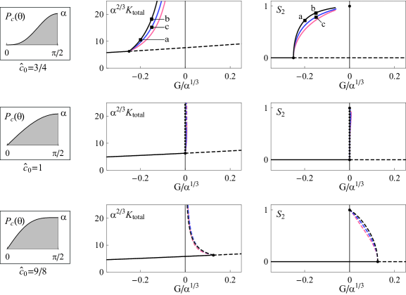
Figure 4: Bifurcation diagrams for the simplified interaction functions using three different induced catastrophe parameters. The figures on the left depict the probability $P_{\textrm{c}}(\theta)$ to induce a catastrophe upon collision, along with the corresponding values of $\hat{c}_{0}$. The centre and right columns depict the corresponding bifurcation diagrams as a function of $G$, expressed in terms of the total density $K_{\textrm{total}}$ and the 2D nematic order parameter $S_{2}$, respectively, where $K_{\textrm{total}}=\int K(\theta)\mathrm{d}\theta$. The isotropic solutions are by definition disordered, so $S_{2}=0$, and their density is computed from (41). The bifurcation point is determined using (49), with $\hat{c}_{2}=-1/2$. For each diagram, ordered solutions have been computed for $\hat{z}_{0}=0$ (black), $\hat{z}_{0}=1$ (blue) and $\hat{z}_{0}=10$ (red). The solutions have been computed using the method discussed in appendix A. Solid lines indicate stable solutions and dashed lines indicate unstable solutions (see also section III.5). Note that the case of $\hat{c}_{0}=1$ in the absence of zippering is a singular case where the stability cannot be determined, because non-isotropic solutions only exist for $G=0$. This has been indicated by a dotted line. The $S_{2}$-diagrams include the asymptotic limit point at $G=0$ with absolute ordering (at infinite density). The labels a, b and c indicate the parameter values of the results depicted in figure 5. The fact that the solutions for $S_{2}$ in the case $\hat{c}_{0}=\frac{3}{4}$ do not reach the asymptotic point $(G=0,S_{2}=1)$ is a consequence of the slowdown in convergence of the path-following method as $G\uparrow 0$.

III.4 Ordered solutions for simplified interaction functions

To find solutions beyond the immediate vicinity of the bifurcation point, we are hampered by the fact that these solutions are part of an infinite-dimensional solution space. In appendix A it is shown that the solutions can be constrained to a finite-dimensional space by restricting the interaction functions $c(\theta)$ and $z(\theta)$ to a finite number of Fourier modes.

In this section, we will define a set of simplified interaction functions by restricting ourselves to Fourier modes up to and including $\cos(4\theta)$. These modes provide us with just enough freedom for the model to exhibit rich behaviour. Using the fact that $c(0)=z(0)=z(\pi/2)=0$, we find that $\hat{z}_{2}=0$ and that both $\hat{z}_{4}$ and $\hat{c}_{4}$ are determined by the remaining parameters. Furthermore, we introduce an overall factor of $\alpha$ in both equations, allowing us to set $\hat{c}_{2}=-1/2$, so that $c(\pi/2)=\alpha$. We thus obtain a system that is fully specified by the parameters $\hat{c}_{0}$, $\hat{z}_{0}$ and $\alpha$.

$$c(\theta) =\alpha\left[\frac{\hat{c}_{0}}{2}-\frac{1}{2}\mathrm{cos}(2\theta)+\frac{1}{2}(1-\hat{c}_{0})\mathrm{cos}(4\theta)\right]$$ (55a)

$$z(\theta) =\alpha\left[\frac{\hat{z}_{0}}{2}(1-\mathrm{cos}(4\theta))\right]$$ (55b)

For $\alpha=1$, $\hat{c}_{0}$ and $\hat{z}_{0}$ are the actual Fourier coefficients of the interaction functions. Demanding that $P_{\textrm{c}}(\theta)=c(\theta)/\mathrm{sin}(\theta)$ is monotonically increasing on the interval $[0,\pi/2]$ leads to the constraint

$$\frac{3}{4}\leq\hat{c}_{0}\leq\frac{9}{8}$$ (56)

and $\hat{z_{0}}$ is a positive real number. Of course, the total probability of zippering and catastrophe induction may not exceed $1$, placing an upper bound on $\alpha$. In the absence of zippering, we have $\alpha\leq 1$.

It should be noted that the value of $\alpha$ has no qualitative effect on the results. This can be understood by realizing that the set of equations (35) is invariant under the substitutions

$$\mathbf{C} \to\alpha\mathbf{C} L \to\alpha^{-1/3}L$$

$$\mathbf{Z} \to\alpha\mathbf{Z} K \to\alpha^{-2/3}K$$

$$G \to\alpha^{1/3}G T \to\alpha^{-1/3}T$$

where the first substitution reflects the presence of $\alpha$ in the definitions (55). The existence of this scaling relation implies that all functional dependencies between any of these parameters and variables remain unchanged when subjected to the inverse scaling. Explicitly, the relevant parameters become $\mathbf{C}/\alpha$, $\mathbf{Z}/\alpha$ and $\alpha^{-1/3}G$ and the variables $\alpha^{1/3}L$, $\alpha^{2/3}K$ and $\alpha^{1/3}T$. With this in mind, we have used the arbitrary choice $\alpha=1$ for our numerical calculations, indicating the appropriate scaling on the axes of figures 4 and 5.

Equation (49) indicates that, for the simplified interaction functions, the bifurcation point is located in the range

$$-\frac{1}{4}\leq G^{*}\leq\frac{1}{8}$$ (57)

and from (41) and (53) we find that $K^{*}=\alpha^{-2/3}$ and $\Lambda^{*}=4/(\alpha\pi)$. We have used the numerical procedure described in appendix A to determine the ordered solutions of (35), starting from the bifurcation point. This has been done for nine different parameter values. For the values of $\hat{c}_{0}$ we used the extreme values $3/4$ and $9/8$, as well as $1$, the latter corresponding to $G^{*}=0$. For each of these three cases, we have varied the zippering parameter $\hat{z}_{0}$, choosing values of $0$, $1$ and $10$. Figure 4 shows the results, depicting both the total density of the system and the degree of ordering as a function of $G$. The degree of ordering is measured by the order parameter $S_{2}$, defined as

$$S_{2}[K(\theta)]=\frac{|\int_{0}^{2\pi}\mathrm{d}\theta\,\mathrm{e}^{i2\theta}K(\theta)|}{\int_{0}^{2\pi}\mathrm{d}\theta\,K(\theta)},$$ (58)

which is the standard 2D nematic liquid crystal order parameter (yielding 0 for a completely disordered system and 1 for a fully oriented system).

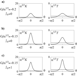
Figure 5: Three stable ordered solutions that correspond to the points labelled (a), (b) and (c) in figure 4. The (unstable) isotropic solutions for the same parameter values are indicated with a dashed line. The parameter values for (a) and (b) differ only in the value of $G$, whereas the parameter values for (b) and (c) differ only in the value of $\hat{z}_{0}$. All results have been calculated using the method described in appendix A.

III.5 Stability of solutions

The bifurcation constraint (46) indicates that the space of bifurcating functions $\kappa_{n}$ is spanned by the functions $\mathrm{cos}(2n\theta)$ and $\mathrm{sin}(2n\theta)$ for a given value of $n\geq 1$. These solutions are therefore symmetric with respect to an arbitrary axis that we choose to place at $\theta=0$. Even after the restriction to this symmetry axis there are still two solution branches emanating from the bifurcation point, differing in the sign of the coefficient of the perturbation. These branches correspond to solutions peaked around $\theta=0$ and $\theta=\pi/(2n)$, respectively, that are identical except for this rotation. The symmetry of these solutions indicates that the bifurcation is of the pitchfork type. In figure 5 we plot the solutions with a maximum at $\theta=0$.

The presence of a pitchfork bifurcation implies a loss of stability of the originating branch [27]. In our system, we know that the isotropic solution must be stable in the limit $G\to-\infty$. Therefore, the local stability of the isotropic solution is lost at the first bifurcation point (for the lowest value of $G$), corresponding to the eigenfunction $\mathrm{cos}(2\theta)$. Because this eigenfunction is orthogonal to the eigenfunctions related to the subsequent bifurcation points ($\mathrm{cos}(2n\theta),n>2$), the stability of the unstable mode will not be regained at any point along the isotropic solution and the isotropic solution itself remains unstable for all higher values of $G$. This also means that the solution branches originating at further pitchfork bifurcations will be unstable near the isotropic solution. In this paper we restrict ourselves to the analysis of the first bifurcation point and the corresponding ordered solution branch. Because the solutions on this branch already have the lowest symmetry permitted by the interaction functions, there are no further bifurcation points along this branch.

Generically [27, chap. IV], the branches of the initial pitchfork bifurcation are stable for a supercritical bifurcation (branches bending towards higher values of $G$) and unstable for a subcritical bifurcation (branches bending towards lower values of $G$). In addition, turning points in the bifurcating branches generally correspond to an exchange of stability [28, page 22]. This analysis allows us to assign stability indicators to the bifurcation diagrams in figure 4, even in the absence of a detailed study of the time-dependent equations (1).

IV Discussion and conclusions

Based on biological observations, we have constructed a model for the orientational alignment of cortical microtubules. The model has a number of striking features. First of all, for a given set of induced catastrophe and zippering probabilities ($P_{\textrm{c}}(\theta)$ and $P_{\textrm{z}}(\theta)$), it allows us to identify a single dimensionless control parameter $G$, which is fully determined by the nucleation rate and intrinsic dynamics of individual microtubules. This result by itself may turn out to be very useful in comparing different in vivo systems or the same system under different conditions or in different developmental stages. For increasing values of $G$, the isotropic stationary solutions to the model show an increase both in density and in abundance of interactions, as measured by the ratio of microtubule length to the mesh-size. Secondly, the bifurcation point, i.e. the critical value of $G^{*}$ of the control parameter at which the system develops ordered stationary solutions from the isotropic state, is determined solely by the probability of collisions between microtubules that lead to an induced catastrophe.

Indeed, from the numerical solutions of the minimal model introduced in Section III.4 it appears, perhaps surprisingly, that the co-alignment of microtubules due to zippering events, if anything, diminishes the degree of order. These results identify the “weeding out” of misaligned microtubules — by marking them for early removal by the induced switch to the shrinking state — as the driving force for the ordering process. Finally, in spite of not being able to directly assess the stability of the solutions in the time-domain, we have provided arguments that stable ordered solutions are possible for the regime $G<0$, i.e. where the length of individual microtubules is intrinsically bounded.

For $G>0$, individual microtubules have the tendency to grow unbounded, unless they are kept in check by catastrophic collisions. Although (locally) stable solutions may exist for values of $G$ that are not too large, for every $G>0$ there exists a class of aligned ‘runaway’ solutions with diverging densities. The computed ordered solutions, regardless of their stability, converge to a point with $G=0$, for which the microtubules are perfectly aligned ($S_{2}=1$) and the system is infinitely dense. The existence of this point can be understood by the fact that the alignment also serves to decrease the number of collisions, and in the limit of a perfectly aligned system, the (relative) number of collisions vanishes.

How realistic is the model presented? To answer this question we need to consider several known factors that have not been included. First of all, microtubules typically can de-attach from their nucleation sites and then perform so called treadmilling motion, whereby the minus-end shrinks at a more or less steady pace, which is small compared to both the growth- and the shrinking speed of the more active plus end. In the case that no zippering occurs at all it is relatively easy to show that the effect of treadmilling simply leads to a renormalization of the parameter $G$ and the interaction functions $c(\theta)$ and $z(\theta)$, but leaving the qualitative behaviour of the model identical to the one discussed here. When zippering does occur, one expects the treadmilling to enhance the degree of ordering in an ordered state, as over time it “eats-up” the, by definition less ordered, initial segments of each microtubule. This effect is also consistent with the observation in figure 5c that in the case with zippering the active tips are on average more strongly aligned than the average segment. In fact, given that the comparison between figures 5b and 5c also shows that, all else being equal, zippering sharpens the orientational distribution of the active tips as compared to the case with no zippering, it is conceivable that the combination of zippering and treadmilling could lead to more strongly ordered systems for the same value of the control parameter.

Next it is known that in vivo severing proteins, such as katanin are active in, and crucial to, the formation of the cortical array [29]. Although in principle the effect of severing proteins could be included in the model, it would present formidable problems in the analysis as well as introduce additional parameters into the model for which precise data is lacking.

Another effect that has not been taken into account explicitly is microtubule bundling. Whenever a microtubule zippers alongside another segment, they form a parallel bundle [30]. However, the coarse-grained nature of our model precludes the formation of bundles and only allows for alignment of the segments. This means that a microtubule that is growing in a different direction encounters each microtubule separately rather than as a single bundle. It is to be expected that the catastrophe and zippering rates stemming from $N$ individual collisions will be higher than those from a single collision with a bundle of $N$ microtubules. Hence, in realistic systems the event rate is likely to be lower than that predicted by the model, or, in other words, corresponds to a lower value of the scaling parameter $\alpha$. Bundles are also thought to be more than just adjacently aligned microtubules, because they may be stabilized through association with bundling proteins that could potentially decrease the catastrophe rate of individual microtubules within a bundle (see [31]). This is a non-trivial effect that should be considered separately and is likely to lead to an increased tendency to form an ordered structure.

Finally, our model implicitly assumes that there is an infinite supply of free tubulin dimers available for incorporation into microtubules. Although there is no definite experimental evidence for this, it is reasonable to assume that in vivo there is a limit to the size of the free tubulin pool. Such a finite tubulin pool would have marked consequences for the behaviour of the model, because the growth speed, and possibly also the nucleation rate, are dependent on the amount of free tubulin, or equivalently the total density of microtubules $k_{tot}$. To a first approximation the growth speed is given by $v^{+}(k_{tot})=v^{+}(k_{tot}=0)\left(1-\frac{k_{tot}}{k_{max}}\right)$ where $k_{max}$ the maximally attainable density when all tubulin is incorporated into microtubules. This allows for stable states to develop even when $G(k_{tot}=0)>0$, because under this pool-size constraint the length of individual microtubules will always remain bounded, and the system will settle into a steady state with $G(k_{tot})<G(k_{tot}=0)$. This behaviour could provide a biologically motivated mechanism by which a solution with a particular density is selected.

To see whether our model, in spite of its approximate nature, makes sense in the light of the available data we first use the collision event probabilities obtained by Dixit and Cyr [15] (see figure 3) to obtain an estimate for the bifurcation value of the control parameter of $G^{*}=-0.15$ for the case of Tobacco BY-2 cells. An ordered phase of cortical microtubules should therefore be possible provided $G>G^{*}$. Given the available data on the microtubule instability parameters in this same system taken from Dhonukshe et al. [10] and Vos et al. [32] we would predict using the definition (35e) that this requires the nucleation rate of new microtubules to be larger than 0.05 min${}^{-1}\mu$m^-2 (Dhonukse) and 0.01 min${}^{-1}\mu$ m^-2 (Vos) respectively. Both these estimates for a lower bound on the nucleation rate are reasonable as they imply the nucleation of order $10^{3}$ microtubules in the whole cortex over the course of the build-up towards full transverse order, comparable to the number that is observed.

Finally, we should point out that our model so far only addresses the question of what causes cortical microtubules to align with respect to each other. Given that in growing plant cells the cortical array is invariably oriented transverse to the growth direction, the question of what determines the direction of the alignment axis with respect to the cell axes is as, if not more, important from a biological perspective. We hope to address this question, as well as the influence of some of the as yet neglected factors mentioned above, in future work.

Appendix A Numerical evaluation of the ordered solutions

The solutions to the set of equations (35) lie in an infinite-dimensional solution space. This creates significant hurdles for the numerical search for solutions. In this section, we will see that it is possible to restrict the solutions to a finite-dimensional space by imposing constraints on the interaction operators $\mathbf{C}$ and $\mathbf{Z}$. In addition, we present a method to follow the branch of ordered solution in this finite-dimensional space, starting from the bifurcation point (49).

We start by reformulating the set of equations (35) by replacing $L(\theta)$ and $T(\theta)$ through the definitions

$$S(\theta) =\frac{1}{L(\theta)}, U(\theta) =\frac{1}{K(\theta)}\left(\frac{T(\theta)}{L(\theta)}-1\right).$$ (59)

Following these substitutions, the interaction operators are all applied at the outermost level of the equations, enabling us to make use of their properties in Fourier space. Explicitly, we obtain

$$S(\theta) =-G+\mathbf{C}\left[K\right]\left(\theta\right)+\mathbf{Z}\left[K\right]\left(\theta\right)$$ (60)

$$Q\left(\theta\right) =\mathbf{Z}\left[K\left(1+Q\right)/S\right]\left(\theta\right)$$ (61)

$$U(\theta) =\mathbf{Z}\left[(1+KU)/S\right](\theta)$$ (62)

and

$$K(\theta) =\frac{1+Q(\theta)}{S^{2}(\theta)-U(\theta)(1+Q(\theta))}.$$ (63)

Denoting the Fourier components of $S(\theta)$, $Q(\theta)$ and $U(\theta)$, by $\hat{s}_{n}$, $\hat{q}_{n}$ and $\hat{u}_{n}$, respectively, the interacting microtubule equations reduce to a (potentially infinite) set of scalar integral equations:

$$\hat{s}_{2n} =-2\delta_{n,0}G+\frac{\hat{c}_{2n}+\hat{z}_{2n}}{\pi}\int_{0}^{2\pi}\mathrm{d}\theta\,\mathrm{cos}(2n\theta)K(\theta)$$ (64a)

$$\hat{q}_{2n} =\frac{\hat{z}_{2n}}{\pi}\int_{0}^{2\pi}\mathrm{d}\theta\,\frac{\mathrm{cos}(2n\theta)K(\theta)\left(1+Q(\theta)\right)}{S(\theta)}$$ (64b)

$$\hat{u}_{2n} =\frac{\hat{z}_{2n}}{\pi}\int_{0}^{2\pi}\mathrm{d}\theta\,\frac{\mathrm{cos}(2n\theta)(1+K(\theta)U(\theta))}{S(\theta)}.$$ (64c)

From the structure of these equations, we immediately see that we can greatly reduce the dimensionality of the problem by setting a number of Fourier coefficients $\hat{z}_{2n}$ and $\hat{c}_{2n}$ to zero. In other words, by restricting our space of interaction functions $c(\theta)$ and $z(\theta)$, the problem can be reduced to a finite number of scalar equations.

Applied to the simplified interaction functions introduced in section III.4, we know that the sets of stationary solutions form lines in the 8-dimensional phase space spanned by the variables $\{\hat{s}_{0},\hat{s}_{2},\hat{s}_{4},\hat{q}_{0},\hat{q}_{4},\hat{u}_{0},\hat{u}_{4}\}$ and the parameter $G$. At least two of such solution lines exist, one corresponding to the isotropic solution and the other to the ordered solution, and these lines intersect at the bifurcation point.

Within this 8-dimensional space, we have used a numerical path-following method similar to the one described in [33, 34] that follows the ordered solution branch by searching for a local minimum in the root mean error of the constituent equations (64). The search for ordered solutions is initiated at the bifurcation point, with coordinates

$$S^{*} =\frac{\hat{z}_{0}-2\hat{c}_{2}}{(-2\hat{c}_{2})^{2/3}}, Q^{*} =-\frac{\hat{z}_{0}}{2\hat{c}_{2}}, U^{*} =\frac{\hat{z}_{0}}{(-2\hat{c}_{2})^{1/3}},$$ (65)

so that in the case of our simplified interaction model

$$\{G,\hat{s}_{0},\hat{s}_{2},\hat{s}_{4},\hat{q}_{0},\hat{q}_{4},\hat{u}_{0},\hat{u}_{4}\}_{0}=\\ \{c_{0}-1,2(\hat{z}_{0}+1),0,0,2\hat{z}_{0},0,2\hat{z}_{0},0\}.$$ (66)

The initial instability affects only the $\mathrm{cos}(2\theta)$ mode. This mode only appears in the equation for $\hat{s}_{2}$ and the remaining parameters are affected only by higher order corrections. For this reason we choose the initial direction of the path to be the unit vector in the $\hat{s}_{2}$-direction and the path is traced from there.

References

- [1] Bruce Alberts, Alexander Johnson, Julian Lewis, Martin Raff, Keith Roberts, and Peter Walter. Molecular Biology of the cell. Garland Science, 4th edition, 2002.
- [2] D.W. Ehrhardt and S.L. Shaw. Microtubule dynamics and organization in the plant cortical array. Annu. Rev. Plant Biol., 57:859–75, 2006.
- [3] A. Paradez, A. Wright, and D.W. Ehrhardt. Microtubule cortical array organization and plant cell morphogenesis. Curr. Opin. Plant Biol., 9(6):571–578, 2006.
- [4] D.J. Cosgrove. Growth of the plant cell wall. Nat. Rev. Mol. Cell Biol., 6:850–861, 2005.
- [5] G.O. Wasteneys and R.E. Williamson. Reassembly of microtubules in nitella tasmanica - quantitative-analysis of assembly and orientation. Eur. J. Cell Biol., 50(1):76–83, 1989.
- [6] F. Kumagai, A. Yoneda, T. Tomida, T. Sano, T. Nagata, and S. Hasezawa. Fate of nascent microtubules organized at the M/G1 interface, as visualized by synchronized tobacco BY-2 cells stably expressing GFP-tubulin: time-sequence observations of the reorganization of cortical microtubules in living plant cells. Plant Cell Physiol., 42(7):723–732, 2001.
- [7] S.L. Shaw, R. Kamyar, and D.W. Ehrhardt. Sustained microtubule treadmilling in Arabidopsis cortical arrays. Science, 300(5626):1715–1718, June 13 2003.
- [8] J.W. Vos, B. Sieberer, A.C.J. Timmers, and A.M.C. Emons. Microtubule dynamics during preprophase band formation and the role of endoplasmic microtubules during root hair elongation. Cell Biol. Int., 27(3):295, 2003.
- [9] A.R. Hardham and B.E. Gunning. Structure of cortical microtubule arrays in plant cells. J. Cell Biol., 77(1):14–34, 1978.
- [10] P. Dhonukshe, A.M. Laxalt, J. Goedhart, T.W.J. Gadella, and T. Munnik. Phospholipase d activation correlates with microtubule reorganization in living plant cells. Plant Cell, 15(11):2666–2679, 2003.
- [11] J.C. Gardiner, J.D. Harper, N.D. Weerakoon, D.A. Collings, S. Ritchie, S. Gilroy, R.J. Cyr, and J. Marc. A 90-kd phospholipase d from tobacco binds to microtubules and the plasma membrane. Plant Cell, 13(9):2143–2158, 2001.
- [12] T. Hashimoto and T. Kato. Cortical control of plant microtubules. Curr. Opin. Plant Biol., 9(1):5–11, 2006.
- [13] T. Hamada. Microtubule-associated proteins in higher plants. J. Plant Res., 120(1):79–98, 2007.
- [14] V. Kirik, U. Herrmann, C. Parupalli, J.C. Sedbrook, D.W. Ehrhardt, and M. Hülskamp. Clasp localizes in two discrete patterns on cortical microtubules and is required for cell morphogenesis and cell division in arabidopsis. J. Cell Sci., 120(24):4416–4425, 2007.
- [15] R. Dixit and R. Cyr. Encounters between dynamic cortical microtubules promote ordering of the cortical array through angle-dependent modifications of microtubule behavior. Plant Cell, 16(12):3274–3284, 2004.
- [16] E. Geigant, K. Ladizhansky, and A. Mogilner. An integro-differential model for orientational distributions of f-actin in cells. SIAM J. Appl. Math, 59:787–809, 1998.
- [17] K. Kruse, J.F. Joanny, F. Jülicher, J. Prost, and K. Sekimoto. Generic theory of active polar gels: a paradigm for cytoskeletal dynamics. Eur. Phys. J. E, 16:5–16, 2005.
- [18] I.S. Aranson and L.S. Tsimring. Theory of self-assembly of microtubules and motors. Phys. Rev. E, 74(3):031915, 2006.
- [19] V. Rühle, F. Ziebert, R. Peter, and W. Zimmermann. Instabilities in a two-dimensional polar-filament-motor system. Eur. Phys. J. E, 27:243–251, 2008.
- [20] A. Zumdieck, M. Cosentino Lagomarsino, C. Tanase, K. Kruse, B.M. Mulder, M. Dogterom, and F. Jülicher. Continuum description of the cytoskeleton: ring formation in the cell cortex. Phys. Rev. Lett., 95(25):258103, 2005.
- [21] V.A. Baulin, C.M. Marques, and F. Thalmann. Collision induced spatial organization of microtubules. Biophys. Chemist., 128:231–244, 2007.
- [22] M. Dogterom and S. Leibler. Physical aspects of the growth and regulation of microtubule structures. Phys. Rev. Lett., 70(9):1347–1350, 1993.
- [23] T. Murata, S. Sonobe, T.I. Baskin, S. Hyodo, S. Hasezawa, T. Nagata, T. Horio, and M. Hasebe. Microtubule-dependent microtubule nucleation based on recruitment of gamma-tubulin in higher plants. Nat. Cell Biol., 7(10):961–968, 2005.
- [24] T. Murata and M. Hasebe. Microtubule-dependent microtubule nucleation in plant cells. J. Plant Res., 120(1):73–78, 2007.
- [25] R.L. Margolis and L. Wilson. Microtubule treadmilling: what goes around comes around. BioEssays, 20:830 – 836, 1998.
- [26] M.E. Janson, M.E. de Dood, and M. Dogterom. Dynamic instability of microtubules is regulated by force. J. Cell Biol., 161(6):1029–1034, 2003.
- [27] M. Golubitsky and D.G. Schaeffer. Singularities and Groups in Bifurcation Theory, volume 1. Springer-Verlag, 1984.
- [28] G. Iooss and D.D. Joseph. Elementary Stability and Bifurcation Theory. Springer-Verlag, 1980.
- [29] A. Roll-Mecak and R.D. Vale. Making more microtubules by severing: a common theme of noncentrosomal microtubule arrays. J. Cell Biol., 175:849–851, 2006.
- [30] D.A. Barton, M. Vantard, and R.L. Overall. Analysis of cortical arrays from Tradescantia virginiana at high resolution reveals discrete microtubule subpopulations and demonstrates that confocal images of arrays can be misleading. Plant Cell, 20:982–994, 2008.
- [31] J. Gaillard, E. Neumann, D. van Damme, V. Stoppin-Mellet, C. Ebel, E. Barbier, D. Geelen, and M. Vantard. Two Microtubule-associated Proteins of Arabidopsis MAP65s Promote Antiparallel Microtubule Bundling. Mol. Biol. Cell, 19(10):4534–4544, 2008.
- [32] J.W. Vos, M. Dogterom, and A.M.C. Emons. Microtubules become more dynamic but not shorter during preprophase band formation: a possible ”search-and-capture” mechanism for microtubule translocation. Cell Motil. Cytoskeleton, 57(4):246–258, 2004.
- [33] E.L. Allgower and K. Georg. Introduction to Numerical Continuation Methods, volume 45 of Classics in Applied Mathematics. SIAM, 2003.
- [34] P. Deuflard, B. Fiedler, and P. Kunkel. Efficient numerical pathfollowing beyond critical points. SIAM J. Numer. Anal., 24(4):912–927, 1987.