Dynamical spin-spin correlation functions in the Kondo model out of equilibrium

Abstract

We calculate the dynamical spin-spin correlation functions of a Kondo dot coupled to two noninteracting leads held at different chemical potentials. To this end we generalize a recently developed real-time renormalization group method in frequency space (RTRG-FS Schoeller09 ) to allow the calculation of dynamical correlation functions of arbitrary dot operators in systems describing spin and/or orbital fluctuations. The resulting two-loop RG equations are analytically solved in the weak-coupling regime. This implies that the method can be applied provided either the voltage $V$ through the dot or the external magnetic field $h_{0}$ are sufficiently large, $\max\{V,h_{0}\}\gg T_{K}$, where the Kondo temperature $T_{K}$ is the scale where the system enters the strong-coupling regime. Explicitly, we calculate the longitudinal and transverse spin-spin correlation and response functions as well as the resulting fluctuation-dissipation ratios. The correlation functions in real-frequency space can be calculated in Matsubara space without the need of any analytical continuation. We obtain analytic results for the line-shape, the small- and large-frequency limits and several other features like the height and width of the peak in the transverse susceptibility at $\Omega\approx\tilde{h}$, where $\tilde{h}$ denotes the renormalized magnetic field. Furthermore, we discuss how the developed method can be generalized to calculate dynamical correlation functions of other operators involving reservoir degrees of freedom as well.

I Introduction

The single-impurity Kondo model Kondo64 is unquestionably one of the most important models studied in condensed matter physics over the past decades. The investigation of its equilibrium properties has caused the development of important theoretical tools such as renormalization group methods or the Bethe Ansatz for impurity systems Wilson75 ; TsvelikWiegmann83 ; Andrei-83 ; Hewson93 . More than 20 years ago it was also realized GlazmanRaikh88 ; NgLee88 ; Kawabata91 that the Kondo model can be used to describe transport experiments through quantum dots. The developments in the ability to engineer devices on the nanoscale has led to the experimental realization of Kondo physics in such systems Goldhaber-98 ; Cronenwett-98 ; Schmid-98 ; Goldhaber-98prl ; Simmel-99 ; Wiel-00 ; Nygard-00 . One particular advantage of these quantum dots is the almost full control over system parameters like temperature, bias and gate voltages, magnetic field, and exchange couplings. These possibilities have triggered a great interest in the theoretical study of quantum dots out of equilibrium. A wide range of theoretical methods has been applied in the past, including non-equilibrium perturbation theory Rosch-01 ; ParcolletHooley02 ; Mao-03 ; ShnirmanMakhlin03 ; Rosch-03prl ; Paaske-04prb1 ; Paaske-04prb2 ; Rosch-05 ; DoyonAndrei06 ; Chung-09 , the flow-equation method Kehrein05 ; Kehreinbook ; FritschKehrein09ap ; FritschKehrein09 , Coulomb gas representations MitraMillis07 ; Segal-07 , real-time and functional renormalization group methods Schoeller00 ; SchoellerKoenig00 ; KeilSchoeller01 ; Jakobs-07 ; Korb-07 ; Schoeller09 ; SchoellerReininghaus09 , a non-equilibrium extension of the numerical renormalization group (NRG) method Anders08prl ; Anders08 , and time-dependent density matrix renormalization group (DMRG) techniques BohrSchmitteckert07 ; Boulat-08 ; Kirino-08 ; Dias-08 ; Heidrich-Meisner-09 . These studies established the importance of relaxation and decoherence effects for the understanding of non-equilibrium physics. From an experimental point of view various measurable quantities like the steady-state current, the magnetization, and the static susceptibility have been calculated.

Beside the application of these techniques there were also attempts to employ the known integrability of certain impurity models in equilibrium, notably the Anderson impurity model and the interacting resonant level model, to investigate their non-equilibrium properties. Konik et al. Konik-01 ; Konik-02 calculated the differential conductance in the Anderson impurity model by combining the well-known scattering states of the equilibrium system TsvelikWiegmann83 with a Landauer-Büttiker formalism. In this work the chemical potentials in the leads were coupled to dressed excitations rather than free electrons and the calculation was restricted to a subset of the excitations. In contrast, a different approach was recently put forward by Metha and Andrei MehtaAndrei06 to treat the interacting resonant level model. They constructed a new set of scattering states of Bethe-Ansatz form which share the quantum numbers of free electrons in the incoming channel, hence allowing the application of a finite voltage in the usual manner. However, questions concerning the existence of these scattering states and issues related to the used regularization scheme of the theory remain open. Nevertheless, the interacting resonant level model has become one of the benchmark systems in the study of non-equilibrium physics Borda-07 ; Doyon07 ; Golub07 ; NishinoHatano07 ; SchillerAndrei07 ; BoulatSaleur08 ; Boulat-08 ; Borda-08 ; Nishino-09 .

Despite the large number of studies of impurity models out of equilibrium only few results are known for the dynamical correlation functions. The spin dynamics of a non-equilibrium quantum dot has been studied by using a Majorana fermion representation Mao-03 ; ShnirmanMakhlin03 , which yields the qualitative low-frequency properties of the correlation functions. The transverse susceptibility in a Kondo model was studied by Paaske et al. Paaske-04prb2 using non-equilibrium perturbation theory together with a pseudo-fermion representation of the Kondo spin. They showed that the Fourier transform of the transverse susceptibility possesses a peak if its frequency equals the value of the applied magnetic field, $\Omega\approx h_{0}$, and that the width of this peak is given by the transverse spin relaxation rate $\tilde{\Gamma}_{2}$. Their derivation was, however, restricted to either the regime $h_{0}\ll\tilde{\Gamma}_{2}$ or $\max\{|\Omega-h_{0}|,\tilde{\Gamma}_{2}\}\ll\max\{h_{0},V\}$, where $V$ denotes the applied voltage. Very recently, Fritsch and Kehrein FritschKehrein09ap ; FritschKehrein09 applied the flow-equation method to study the longitudinal correlation function as well as the magnetization and T-matrix in a Kondo model in and out of equilibrium. The numerical solution of the two-loop scaling equations allowed them to study the correlation function for all combinations of the parameters voltage, temperature, and magnetic field, provided the weak-coupling condition (i.e. the presence of a large enough infrared cutoff) was satisfied. In particular, these numerical solutions were used to compare the effects of an applied voltage and a finite temperature, revealing qualitative differences such as the appearance of Kondo splitting in the non-equilibrium situation. In general, however, this method cannot provide analytic expressions for the line shape.

In this article we will generalize the real-time renormalization group method in frequency space Schoeller09 to allow the calculation of dynamical correlation functions of arbitrary dot operators in systems describing spin and/or orbital fluctuations. In this setting the quantum dot is coupled to non-interacting leads which are held at different chemical potentials. The derived two-loop RG equations can be solved analytically in the weak-coupling regime. Explicitly, we calculate the longitudinal and transverse spin-spin correlation and response functions in a two-lead Kondo model in a magnetic field $h_{0}$ up to order $J_{c}^{2}$. Here $J_{c}$ denotes the effective coupling at the energy scale $\Lambda_{c}=\max\{V,h_{0}\}$ where the flow of the coupling constant is cut-off. In order to satisfy the weak-coupling condition $J_{c}\ll 1$ either the applied voltage or the magnetic field have to be sufficiently large compared to the Kondo temperature, $\Lambda_{c}\gg T_{K}$, where $T_{K}$ is the scale where the system enters the strong-coupling regime. We note that the applied formalism does not rely on a fermionic representation of the Kondo spin but rather deals with its matrix representation in Liouville space directly. The longitudinal response function possesses a peak at the spin relaxation rate $\tilde{\Gamma}_{1}$, which gets suppressed in a finite magnetic field. Interestingly, in the case of a strong magnetic field, $V<\tilde{h}$ where $\tilde{h}=(1-J_{c}+\ldots)h_{0}$ denotes the renormalized magnetic field (see Eq. (182) for the precise value), the longitudinal correlation and response function show “kink-like” structures at the frequencies $\Omega=\tilde{h},\tilde{h}\pm V$, which were also observed using the flow-equation method FritschKehrein09 . Here we additionally provide the line shape close to these “kinks” and show that the real part of the response functions shows characteristic logarithmic features at $\Omega=\tilde{h},\tilde{h}\pm V$. Furthermore we study the longitudinal and transverse fluctuation-dissipation ratios. As expected these ratios show a revival of the fluctuation-dissipation theorem CallenWelton51 ; Landau5 provided the applied voltage is small compared to the magnetic field or the considered oscillation frequency.

This article is organized as follows. In the next two sections we will define the general set up we want to study and define the used notations. This will include the Kondo model, the notion of Liouville operators as well as the definition of the symmetrized correlation function and susceptibility. In Sec. IV we will then derive perturbative expansions for the kernels needed to calculate these correlation functions. This will be performed in Liouville space; the expansion is done in powers of the exchange coupling between the dot and the reservoirs. These perturbative expansions can be applied to any model describing spin and/or orbital fluctuations as well as correlation functions of arbitrary operators. In Sec. V we will use these results to derive the RG equations for the kernels of pure dot operators. In the following section we will further specialize to the two-lead Kondo model, where we use the explicit expressions of the Liouville operator and the coupling between the dot and the reservoirs to derive analytic results for the effective kernels appearing in the correlation functions. Finally, these expressions for the kernels are used in Secs. VII and VIII to calculate the longitudinal and transverse correlation and response functions.

II Kondo model

The real-time renormalization group in frequency space was applied in Ref. SchoellerReininghaus09, to calculate various quantities including the spin relaxation and dephasing rates, the renormalized magnetic field, the magnetization and the current in the anisotropic Kondo model in a finite magnetic field out of equilibrium. In this reference all notations which we will use in the following were originally set up. In order to increase the readability of the present manuscript we will briefly recall the basic formulas and notations.

We consider a quantum dot with fixed charge in the Coulomb blockade regime coupled to external reservoirs. As shown in detail in Ref. Korb-07, , a standard Schrieffer-Wolff transformation leads to a Hamiltonian of the form

$$H\,=\,H_{res}\,+\,H_{S}\,+\,V\,=\,H_{0}\,+\,V,$$ (1)

where $H_{res}$ is the reservoir part, $H_{S}$ characterizes the isolated quantum dot, and $V$ describes the coupling between reservoirs and quantum dot. They are given explicitly by

$$H_{res}\, = \,\sum_{\nu\equiv\alpha\sigma\dots}\int d\omega\,(\omega+\mu_{\alpha})\,a_{+\nu}(\omega)a_{-\nu}(\omega),$$ (2)

$$H_{S}\, = \,\sum_{s}\,E_{s}\,|s\rangle\langle s|,$$ (3)

$$V\, = \,{1\over 2}\,\sum_{\eta\eta^{\prime}}\sum_{\nu\nu^{\prime}}\int d\omega\int d\omega^{\prime}\,g_{\eta\nu,\eta^{\prime}\nu^{\prime}}(\omega,\omega^{\prime})$$ (4)

$$\hskip 56.9055pt\,\times:a_{\eta\nu}(\omega)\,a_{\eta^{\prime}\nu^{\prime}}(\omega^{\prime}):.$$

Here, $a_{\eta\nu}$ are the fermionic creation ($\eta=+$) and annihilation ($\eta=-$) operators in the reservoirs and $\nu$ is an index characterizing all quantum numbers of the reservoir states, which contains the reservoir index $\alpha\equiv L,R\equiv\pm$ and the spin quantum number $\sigma\equiv\uparrow,\downarrow\equiv\pm$. We measure the energy $\omega$ of the reservoir states relative to the chemical potential $\mu_{\alpha}$ of reservoir $\alpha$. The eigenstates and eigenenergies of the isolated quantum dot are denoted by $\left|s\right\rangle$ and $E_{s}$. The interaction $V$ is quadratic in the reservoir field operators, which arises from second order processes of one electron hopping on and off the quantum dot coherently. This keeps the charge fixed and allows only spin/orbital fluctuations. The coupling vertex $g_{\eta\nu,\eta^{\prime}\nu^{\prime}}(\omega,\omega^{\prime})$ is an arbitrary operator acting on the dot states. It is written in its most general form, depending on the quantum numbers and energies of the reservoir states in an arbitrary way. As explained in Ref. Schoeller09, , the RG approach can be set up in its most convenient form if one assumes that the frequency dependence of the initial vertices is rather weak and varies on the scale of the band width $D$ of the reservoirs. For the model we have in mind, the isotropic spin-$\tfrac{1}{2}$ Kondo model in a magnetic field, this is certainly satisfied. Therefore, we will assume this in the following and introduce below [see Eq. (14)] a convenient cutoff function into the free reservoir Green’s functions.

To achieve a more compact notation for all indices, we write $1\equiv\eta\nu\omega$ and sum (integrate) implicitly over all indices (frequencies). The interaction is then written in the compact form

$$V\,=\,{1\over 2}\,g_{11^{\prime}}\,:a_{1}a_{1^{\prime}}:.$$ (5)

$:\dots:$ denotes normal-ordering of the reservoir field operators, meaning that no contraction is allowed between reservoir field operators within the normal-ordering. Within the normal-ordering of Eq. (5), the field operators can be arranged in an arbitrary way (up to a fermionic sign), therefore the coupling vertex can always be chosen such that antisymmetry holds:

$$g_{11^{\prime}}\,=\,-\,g_{1^{\prime}1}.$$ (6)

Furthermore, due to the hermiticity of $V$, the vertex has the property

$$g_{11^{\prime}}^{\dagger}\,=\,g_{\bar{1}^{\prime}\bar{1}},$$ (7)

where $\bar{1}\equiv-\eta,\nu,\omega$.

Figure 1: Isotropic spin-1/2 Kondo model coupled via exchange to two reservoirs. $J_{LL}$ and $J_{RR}$ involve exchange between the electron spins of the left/right reservoir and the local spin, $J_{RL}=J_{LR}$ transfers an electron from one reservoir to the other during the exchange process. We assume that the Kondo model was derived from an Anderson impurity model via a Schrieffer-Wolff transformation, which implies the relation $J_{LL}\,J_{RR}=J_{RL}^{2}$.

The specific model we want to study is the isotropic Kondo model in an external magnetic field $h_{0}>0$ (see Fig. 1). In this case the above relations read explicitly

$$H_{S} = h_{0}\,S^{z},$$ (8)

$$g_{11^{\prime}} = {1\over 2}\left\{\begin{array}[]{ll}(J_{\alpha\alpha^{\prime}})_{0}S^{i}\sigma^{i}_{\sigma\sigma^{\prime}}&\text{for $\eta=-\eta^{\prime}=+$}\\[5.69054pt] -(J_{\alpha^{\prime}\alpha})_{0}S^{i}\sigma^{i}_{\sigma^{\prime}\sigma}&\text{for $\eta=-\eta^{\prime}=-$}\end{array}\right.\,,$$ (11)

where $i\in\{x,y,z\}$, $S^{i}$ is the $i$-component of the spin-$\tfrac{1}{2}$ operator of the quantum dot, $\sigma^{i}$ is a Pauli matrix, and $(J_{\alpha\alpha^{\prime}})_{0}$ are the initial exchange couplings. We will be interested in the antiferromagnetic model here, i.e., we assume $(J_{\alpha\alpha^{\prime}})_{0}>0$ initially. If one derives the Kondo model via a Schrieffer-Wolff transformation from an Anderson impurity model (see, e.g., Ref. Korb-07, ), one further finds

$$(J_{\alpha\alpha^{\prime}})_{0}\,=\,2\sqrt{x_{\alpha}x_{\alpha^{\prime}}}\,J_{0},\quad\sum_{\alpha}\,x_{\alpha}\,=\,1.$$ (12)

Although the general formalism and many of the following formulas are also valid for an arbitrary number of reservoirs, we will consider the case of two reservoirs only with chemical potentials given by

$$\mu_{L}={V\over 2},\quad\mu_{R}=-{V\over 2},$$ (13)

where $V$ is the applied voltage which we assume to be positive, $V>0$.

A contraction is defined with respect to a grand-canonical distribution of the reservoirs, given by

$${a_{1}\,a_{1^{\prime}}\begin{picture}(-20.0,11.0)\put(-22.0,8.0){\line(0,1){3.0}} \put(-22.0,11.0){\line(1,0){12.0}} \put(-10.0,8.0){\line(0,1){3.0}} \end{picture}\begin{picture}(20.0,11.0)\end{picture}}\,\equiv\,\langle a_{1}a_{1^{\prime}}\rangle_{\rho_{res}}\,=\,\delta_{1\bar{1}^{\prime}}\,\rho(\omega)\,f_{\alpha}(\eta\omega).$$ (14)

$f_{\alpha}(\omega)=(e^{\omega/T_{\alpha}}+1)^{-1}=1-f_{\alpha}(-\omega)$ is the Fermi distribution function corresponding to temperature $T_{\alpha}$ (note that the chemical potential does not enter this formula since $\omega$ is measured relative to $\mu_{\alpha}$). Furthermore, $\delta_{11^{\prime}}\equiv\delta_{\eta\eta^{\prime}}\delta_{\nu\nu^{\prime}}\delta(\omega-\omega^{\prime})$ is the $\delta$-function in compact notation. Furthermore, we have introduced the cutoff by the band width $D$ into the reservoir contraction via the density of states

$$\rho(\omega)\,=\,{D^{2}\over D^{2}+\omega^{2}}.$$ (15)

In order to calculate the dynamical spin-spin correlation functions we have to know the time evolution of the density matrix $\rho(t)$. Formally, this follows from the solution of the von Neumann equation

$$\rho(t) = e^{-\text{i}H(t-t_{0})}\,\rho(t_{0})\,e^{\text{i}H(t-t_{0})}$$ (16)

$$= e^{-\text{i}L(t-t_{0})}\,\rho(t_{0}),$$

where

$$L\,=\,\left[H,.\right]_{-},$$ (17)

is the Liouvillian acting on usual operators in Hilbert space via the commutator. The form (1) of the Hamiltonian yields a similar decomposition of the Liouvillian,

$$L=L_{res}+L_{S}^{(0)}+L_{V},$$ (18)

with $L_{res}=\left[H_{res},.\right]_{-}$, $L_{S}^{(0)}=\left[H_{S},.\right]_{-}$, and $L_{V}=\left[H_{V},.\right]_{-}$. We would like to note that the concept of Liouville space and superoperators have been used in various contexts, for example in quantum statistical mechanics FickSauermann ; Lawrie94 .

Initially, we assume that the density matrix is a product of an arbitrary dot part $\rho_{S}(t_{0})$ and a grandcanonical distribution $\rho_{res}$ for the reservoirs,

$$\rho(t_{0})=\rho_{S}(t_{0})\,\rho_{res}.$$ (19)

Furthermore, we introduce the Laplace transform

$$\tilde{\rho}(z)=\int_{t_{0}}^{\infty}dt\,e^{\text{i}z(t-t_{0})}\,\rho(t)={\text{i}\over z-L}\,\rho(t_{0}),$$ (20)

where we will frequently use the notation $z=E+\text{i}\omega$. The stationary density matrix is defined as

$$\rho^{st}=\lim_{t\rightarrow\infty}\rho(t)=\lim_{t_{0}\rightarrow-\infty}\rho(t),$$ (21)

which is understood in the sense $\mbox{Tr}(O\rho^{st})=\lim_{t\rightarrow\infty}\mbox{Tr}(O\rho(t))$ for any local operator $O$, and can be calculated using

$$\rho^{st}=-\text{i}\lim_{z\rightarrow\text{i}0+}\,z\,\tilde{\rho}(z)=\lim_{z\rightarrow\text{i}0+}\frac{z}{z-L}\rho(t_{0}).$$ (22)

The existence of a stationary state was proven in Ref. DoyonAndrei06, using non-equilibrium pertubation theory to all orders as well as in Ref. Schoeller09, using the RTRG-FS, which in particular clarified the generation of the relaxation and dephasing rates under the RG flow. The reduced density matrix of the dot is obtained by tracing out the reservoir degrees of freedom

$$\tilde{\rho}_{S}(z)=\mbox{Tr}_{res}\,\tilde{\rho}(z)={\text{i}\over z-L_{S}^{eff}(z)}\,\rho_{S}(t_{0}),$$ (23)

where $L_{S}^{eff}(z)$ denotes the effective Liouvillian of the quantum dot formally defined in (63) below. The stationary reduced density matrix can then be obtained similar to (22),

$$\rho_{S}^{st}=\lim_{t\rightarrow\infty}\rho_{S}(t)=\lim_{z\rightarrow\text{i}0+}\frac{z}{z-L_{S}^{eff}(z)}\,\rho_{S}(t_{0}).$$ (24)

III Correlation functions

The quantities of interest in this article are the two-point correlation function of two operators $A$ and $B=A^{\dagger}$ as well as their dynamical susceptibility with respect to the steady state,

$$S_{AB}(t)\! = \!\frac{1}{2}\Bigl{\langle}\left[A(t)_{\mathrm{H}}\!-\!\bigl{\langle}A\bigr{\rangle}_{st},B(0)_{\mathrm{H}}\!-\!\bigl{\langle}B\bigr{\rangle}_{st}\right]_{+}\Bigr{\rangle}_{st},\qquad$$ (25)

$$\chi_{AB}(t)\! = \!\text{i}\,\Theta(t)\Bigl{\langle}\left[A(t)_{\mathrm{H}},B(0)_{\mathrm{H}}\right]_{-}\Bigr{\rangle}_{st}.$$ (26)

where

$$\bigl{\langle}O\bigr{\rangle}_{st}=\lim_{t_{0}\rightarrow-\infty}\mbox{Tr}\Bigl{(}O\,e^{\text{i}Lt_{0}}\,\rho(t_{0})\Bigr{)}=\lim_{t_{0}\rightarrow-\infty}\mbox{Tr}\Bigl{(}O\,\rho(0)\Bigr{)}.$$ (27)

Here the trace is taken over the dot states as well as the reservoir degrees of freedom, $\mbox{Tr}=\mbox{Tr}_{S}\,\mbox{Tr}_{res}$. The time-evolution of the operators in the Heisenberg picture is given by

$$A(t)_{\mathrm{H}}=e^{\text{i}Ht}\,A\,e^{-\text{i}Ht}=e^{\text{i}Lt}\,A.$$ (28)

Instead of calculating (25) and (26) in real time we will study their respective Fourier transforms

$$S_{AB}(\Omega) = \int_{-\infty}^{\infty}dt\,e^{\text{i}\Omega t}\,S_{AB}(t),$$ (29)

$$\chi_{AB}(\Omega) = \int_{-\infty}^{\infty}dt\,e^{\text{i}\Omega t}\,\chi_{AB}(t),$$ (30)

where $\Omega=\Omega\pm\text{i}\delta$ for $t>0$ ($t<0$). The susceptibility admits the standard decomposition $\chi_{AB}(\Omega)=\chi_{AB}^{\prime}(\Omega)+\text{i}\,\chi_{AB}^{\prime\prime}(\Omega)$.

In order to calculate $S_{AB}(\Omega)$ and $\chi_{AB}(\Omega)$ we introduce the auxiliary correlation functions

$$C^{\pm}_{AB}(\Omega)=\int_{-\infty}^{0}dt\,e^{-\text{i}\Omega t}\,\Bigl{\langle}\left[A(0)_{\mathrm{H}},B(t)_{\mathrm{H}}\right]_{\pm}\Bigr{\rangle}_{st}$$ (31)

with $\Omega=\Omega+\text{i}\delta$. Its relations to the correlation functions are given by (see App. A)

$$S_{AB}(\Omega) = Re\,C^{+}_{AB}(\Omega)-2\pi\,\bigl{\langle}A\bigr{\rangle}_{st}\bigl{\langle}B\bigr{\rangle}_{st}\,\delta(\Omega),\quad$$ (32)

$$\chi_{AB}(\Omega) = \text{i}\,C^{-}_{AB}(\Omega).$$ (33)

The static susceptibility is related to the dynamical susceptibility via

$$\chi_{AB}=\frac{\partial M}{\partial h_{0}}=-\lim_{\Omega\rightarrow 0}\,\chi_{AB}^{\prime}(\Omega),$$ (34)

where $M=\langle S^{z}\rangle_{st}$ denotes the magnetization.

Some general properties of the correlation functions can be obtained by considering their spectral representations. Let $\{\left|n\right\rangle\}$ be a complete set of basis states of the full Hamiltonian $H$, i.e. $H\left|n\right\rangle=E_{n}\left|n\right\rangle$. Furthermore, the stationary density matrix $\rho^{st}$ satisfies $\left[H,\rho^{st}\right]_{-}=0$, thus the basis states $\left|n\right\rangle$ can be chosen such that

$$\left\langle n\right|\rho^{st}\left|m\right\rangle=\rho_{n}^{st}\,\delta_{nm}.$$ (35)

Using this one easily verifies the spectral representations

$$C^{\pm}_{AB}(\Omega) = \sum_{mn}(\rho_{n}^{st}\pm\rho_{m}^{st})\,\left\langle n\right|A\left|m\right\rangle\,\left\langle m\right|B\left|n\right\rangle$$ (36)

$$\!\!\!\!\!\!\!\!\!\!\!\!\!\!\!\!\!\!\!\!\times\left(\pi\delta(\Omega+E_{n}-E_{m})+\text{i}\frac{\text{P}}{\Omega+E_{n}-E_{m}}\right).\quad$$

These relations imply $S_{AA^{\dagger}}(\Omega)\geq 0$ as well as $S_{BA}(\Omega)=S_{AB}(-\Omega)$, $\chi_{BA}^{\prime}(\Omega)=\chi_{AB}^{\prime}(-\Omega)$, and $\chi_{BA}^{\prime\prime}(\Omega)=-\chi_{AB}^{\prime\prime}(-\Omega)$. In equilibrium the matrix elements of the density matrix are given by $\rho_{n}=e^{-E_{n}/T}/Z$ with the partition sum $Z$, which implies the well-known fluctuation-dissipation theorem CallenWelton51 ; Landau5

$$\chi_{AA^{\dagger}}^{\prime\prime}(\Omega)=\tanh\frac{\Omega}{2T}\,S_{AA^{\dagger}}(\Omega)$$ (37)

as well as $\Omega\,\chi_{AA^{\dagger}}^{\prime\prime}(\Omega)\geq 0$.

IV Perturbative expansion for the correlation functions

In this section we derive a perturbative expansion in Liouville space for the auxiliary correlation functions $C^{\pm}_{AB}(\Omega)$, which will serve as the starting point for the derivation of the RG equations below. A similar perturbative expansion for the effective Liouvillian of the quantum dot $L_{S}^{eff}$ has been derived in Refs. Schoeller09, ; SchoellerReininghaus09, . We will generalize these results to $C^{\pm}_{AB}(\Omega)$ while closely following the presentation of Ref. SchoellerReininghaus09, .

As starting point to set up the formalism we assume that the operators $A$ and $B$ admit a representation similar to (5),

$$A=\frac{1}{m!}\,a_{1\ldots m}\,:a_{1}\ldots a_{m}:,\quad B=\frac{1}{n!}\,b_{1\ldots n}\,:a_{1}\ldots a_{n}:,$$ (38)

where we recall the short-hand notation $1\equiv\eta\nu\omega$ and sum (integrate) implicitly over all indices (frequencies). We further assume the operators $A$ and $B$ to be bosonic which implies $m$ and $n$ to be even. Eventually we will be concerned with the correlation functions of the spin operators on the dot, i.e. $A,B=S^{+},S^{-},S^{z}$. In this case the operators do not couple dot and reservoir degrees of freedom and hence only the terms with $m=n=0$ are non-vanishing. However, we will keep the general forms (38) throughout this section, which for example include the case of current operators Schoeller09 ; SchoellerReininghaus09 where $m=n=2$.

In order to set up the perturbative expansions in Liouville space we define the operators

$$L_{A}=\frac{\text{i}}{2}\left[A,.\right]_{+},\quad L_{B}^{\pm}=\text{i}\left[B,.\right]_{\pm}.$$ (39)

Then using (28) together with (16) we obtain after some algebra

$$\begin{split}C^{\pm}_{AB}(\Omega)=&(-\text{i})^{2}\lim_{t_{0}\rightarrow-\infty}\,\int_{-\infty}^{0}\,dt\,e^{-\text{i}\Omega t}\\ &\times\mbox{Tr}\left(L_{A}\,e^{\text{i}Lt}\,L_{B}^{\pm}\,e^{-\text{i}L(t-t_{0})}\,\rho(t_{0})\right).\end{split}$$ (40)

In the next step we use (21) and (22) and furthermore perform the Laplace transform $t\rightarrow\Omega$ in (40) to obtain

$$C^{\pm}_{AB}(\Omega)=-\text{i}\lim_{\xi\rightarrow\text{i}0+}\,\mbox{Tr}\left(L_{A}\,\frac{1}{\Omega-L}\,L_{B}^{\pm}\,\frac{\xi}{\xi-L}\,\rho(t_{0})\right).$$ (41)

Here we have used $\Omega=\Omega+\text{i}\delta$ to ensure convergence of the integral. The limit $\xi\rightarrow\text{i}0+$ has to be taken before $\delta\rightarrow 0$ in order to reach the stationary state.

The next step is to expand the expression (41) in the interacting part $L_{V}$ of the Liouvillian and to integrate out the reservoir part. This procedure was outlined for the reduced density matrix $\tilde{\rho}_{S}(z)$ in detail in Ref. Schoeller09, ; we will generalize this to the case of the auxiliary correlation functions (41) here. First, using $L=L_{0}+L_{V}$ with $L_{0}=L_{res}+L_{S}^{(0)}$, (41) can be formally expanded in $L_{V}$,

$$\begin{split}C^{\pm}_{AB}(\Omega)=&-\text{i}\!\lim_{\xi\rightarrow\text{i}0+}\!\sum_{k,l=0}^{\infty}\!\mbox{Tr}\Biggl{[}L_{A}\,\frac{1}{\Omega-L_{0}}\left(L_{V}\,\frac{1}{\Omega-L_{0}}\right)^{k}\\ &\times L_{B}^{\pm}\,\frac{\xi}{\xi-L_{0}}\,\left(L_{V}\,\frac{1}{\xi-L_{0}}\right)^{l}\,\rho(t_{0})\Biggr{]}.\end{split}$$ (42)

Second, in order to integrate out the reservoir degrees of freedom we write $L_{V}$ in the form

$$L_{V}\,=\,{1\over 2}\,p^{\prime}\,G^{pp^{\prime}}_{11^{\prime}}\,:J^{p}_{1}J^{p^{\prime}}_{1^{\prime}}:,$$ (43)

where we implicitly sum (integrate) over $1=\eta\nu\omega$ as well as $p,p^{\prime}=\pm$. $J^{p}_{1}$ is a quantum field superoperator in Liouville space for the reservoirs, defined by ($C$ is an arbitrary reservoir operator)

$$J_{1}^{p}\,C\,=\,\left\{\begin{array}[]{cl}a_{1}\,C&\mbox{for }p=+\\ C\,a_{1}&\mbox{for }p=-\end{array}\right..$$ (44)

Here $p=\pm$ serves as an auxiliary index which is similar to the Keldysh index indicating whether the field operator is acting on the upper or the lower part of the Keldysh contour. $G^{pp^{\prime}}_{11^{\prime}}$ is a superoperator acting in Liouville space of the quantum dot, and is defined by ($C$ is an arbitrary operator on the quantum dot)

$$G^{pp^{\prime}}_{11^{\prime}}\,C\,=\,\delta_{pp^{\prime}}\,\left\{\begin{array}[]{cl}g_{11^{\prime}}\,C&\mbox{for }p=+\\ -C\,g_{11^{\prime}}&\mbox{for }p=-\end{array}\right..$$ (45)

In the same way we define

$$L_{A} = \frac{1}{m!}\,\sigma^{p_{1}\ldots p_{m}}\,\mathcal{A}^{p_{1}\ldots p_{m}}_{1\ldots m}\,:J_{1}^{p_{1}}\ldots J_{m}^{p_{m}}:,$$ (46)

$$L_{B}^{\pm} = \frac{1}{n!}\,\sigma^{p_{1}\ldots p_{n}}\,\mathcal{(B_{\pm})}^{p_{1}\ldots p_{n}}_{1\ldots n}\,:J_{1}^{p_{1}}\ldots J_{n}^{p_{n}}:,$$ (47)

where the dot superoperators $\mathcal{A}^{p_{1}\ldots p_{m}}_{1\ldots m}$ and $\mathcal{(B_{\pm})}^{p_{1}\ldots p_{n}}_{1\ldots n}$ act on arbitrary dot operators $C$ as

$$\mathcal{A}^{p_{1}\ldots p_{m}}_{1\ldots m}\,C = \frac{\text{i}}{2}\,\delta_{p_{1}p_{2}}\ldots\delta_{p_{1}p_{m}}$$ (50)

$$\quad\times\left\{\begin{array}[]{ll}a_{1\ldots m}\,C,&p_{1}=+\\ C\,a_{1\ldots m},&p_{1}=-\end{array}\right.,$$

$$\mathcal{(B_{\pm})}^{p_{1}\ldots p_{n}}_{1\ldots n}\,C = \text{i}\,\delta_{p_{1}p_{2}}\ldots\delta_{p_{1}p_{n}}$$ (53)

$$\quad\times\left\{\begin{array}[]{ll}b_{1\ldots n}\,C,&p_{1}=+\\ \pm C\,b_{1\ldots n},&p_{1}=-\end{array}\right..$$

For $m=0$ or $n=0$ we define $\mathcal{A}C=\frac{\text{i}}{2}\left[a,C\right]_{+}$ and $\mathcal{B_{\pm}}C=\text{i}\left[b,C\right]_{\pm}$, respectively. As we consider only bosonic operators $A$ and $B$ which change the number of fermions by an even integer, the sign-superoperator is given by

$$\sigma^{p_{1}\ldots p_{n}}=p_{2}\,p_{4}\cdots p_{n}.$$ (54)

This operator was introduced to compensate additional signs due to interchanges of fermionic reservoir field operators as explained in detail in Ref. Schoeller09, .

Inserting the representations (43) as well as (46) and (47) into (42) and shifting all reservoir field superoperators $J_{1}^{p}$ to the right using

$$J_{1}^{p}\,L_{res}=(L_{res}-x_{1})\,J_{1}^{p},$$ (55)

where we have introduced the short-hand notation $x_{i}=\eta_{i}(\omega_{i}+\mu_{\alpha_{i}})$, one can showSchoeller09 that each term of perturbation theory can be written as a product of a dot part and an average over a sequence of field superoperators of the reservoirs with respect to $\rho_{res}$. Evaluating the latter with the help of Wick’s theorem, one can represent each term of the Wick decomposition by a diagram (see Fig. 2 for an example) describing a certain process contributing to the auxiliary correlation function $C^{\pm}_{AB}(\Omega)$. Each process consists of a sequence of interaction vertices $G_{11^{\prime}}^{pp^{\prime}}$ between the dot and the reservoirs, and a free time propagation of the dot in between (leading to resolvents in Laplace space). Since the reservoirs have been integrated out, the vertices are connected by reservoir contractions (the green lines in Fig. 2). This means that the various diagrams represent terms for the effective time evolution of the dot in the presence of dissipative reservoirs.

\psfrag{Avertex}{$\mathcal{A}_{12}$}\psfrag{Bvertex}{$\mathcal{B}_{\pm,78}$}\includegraphics[scale={0.28}]{diagram_example.eps}

Figure 2: (color online) Example of a diagram contributing to the auxiliary correlation function $C^{\pm}_{AB}(\Omega)$. The time direction is to the left. Each vertex $G$ is represented by two adjacent black dots indicating the two reservoir field operators associated with each vertex. The vertices $\mathcal{A}$ and $\mathcal{B}$ are represented in the same way by red dots. For this example we have chosen $m=n=2$ in (38) as it would be the case for a current-current correlation function. The black horizontal lines connecting the vertices denote the free time propagation of the quantum system, leading to the resolvents ${1\over E+X_{i}-L_{S}^{(0)}}$ in Laplace space. The green lines are the reservoir contractions arising from the application of Wick’s theorem. The vertical blue lines between the vertices are auxiliary lines to determine the energy argument $X_{i}$ of the resolvents.

Each diagram for the auxiliary correlation function has the form

$$C^{\pm}_{AB}(\Omega) \,\rightarrow\, -{\text{i}\over S}\,(-1)^{N_{p}}\,\left(\prod\gamma\right)\lim_{\xi\rightarrow\text{i}0+}\xi$$ (56)

$$\mathcal{A}\,{1\over\Omega+X_{1}-L_{S}^{(0)}}\,G\,{1\over\Omega+X_{2}-L_{S}^{(0)}}\,\,G\,\dots\,\mathcal{B}_{\pm}$$

$$\ldots\,G\,{1\over\xi+X_{r}-L_{S}^{(0)}}\,G\,{1\over\xi-L_{S}^{(0)}}\,\rho_{S}(t_{0}),$$

where $L_{S}^{(0)}=\left[H_{S},.\right]_{-}$, $G\equiv G_{ij}^{p_{i}p_{j}}$ indicates an interaction vertex, and $\gamma\equiv\gamma^{p_{i}p_{j}}_{ij}$ is a contraction between the reservoir field superoperators, defined by

$$\gamma_{11^{\prime}}^{pp^{\prime}}\, = \,{J_{1}^{p}\,J_{1^{\prime}}^{p^{\prime}}\begin{picture}(-20.0,11.0)\put(-22.0,8.0){\line(0,1){3.0}} \put(-22.0,11.0){\line(1,0){12.0}} \put(-10.0,8.0){\line(0,1){3.0}} \end{picture}\begin{picture}(20.0,11.0)\end{picture}}\,=\,p^{\prime}\,\mbox{Tr}_{res}\,J_{1}^{p}J_{1^{\prime}}^{p^{\prime}}\,\rho_{res}$$

$$= \,\delta_{1\bar{1}^{\prime}}\,\rho(\omega)\,p^{\prime}\,f_{\alpha}(\eta p^{\prime}\omega).$$ (57)

We stress that only the initial reduced density matrix of the dot $\rho_{S}(t_{0})$ defined in (19) appears in (56) as we have already performed the trace over the reservoir degrees of freedom (and hence $\rho_{res}$) to obtain the reservoir contractions $\gamma$. To factorize the Wick decomposition, a fermionic sign has to be assigned to each permutation of reservoir field superoperators, indicated by the sign factor $(-1)^{N_{p}}$ in (56). For each pair of vertices connected by two reservoir lines, a combinatorial factor ${1\over 2}$ occurs, leading to the prefactor ${1\over S}$ in (56). The value of the frequencies $X_{i}$ in the resolvents between the interaction vertices is determined by the sum over all variables $x=\eta(\omega+\mu_{\alpha})$ of those indices belonging to the reservoir lines which are crossed by a vertical line at the position of the resolvent (the blue lines in Fig. 2). Thereby, the index of the left vertex has to be taken of the corresponding reservoir line. For example, the diagram shown in Fig. 2 is given by (the obvious dependence on the Keldysh indices has been omitted for simplicity, i.e. $\gamma_{ij}\equiv\gamma_{ij}^{p_{i}p_{j}}$ and $G_{ij}\equiv G_{ij}^{p_{i}p_{j}}$)

$$\begin{split}&-\text{i}\lim_{\xi\rightarrow\text{i}0+}\xi\Bigl{(}\gamma_{16}\gamma_{23}\gamma_{45}\,\mathcal{A}_{12}\,\Pi_{12}(\Omega)\,G_{34}\,\Pi_{14}(\Omega)\,G_{56}\Bigr{)}\\ &\quad\times{1\over\Omega-L_{S}^{(0)}}\left({1\over 2}\gamma_{7,10}\gamma_{89}\,\mathcal{B}_{\pm,78}\,\Pi_{78}(\xi)\,G_{9,10}\right)\\ &\quad\times{1\over\xi-L_{S}^{(0)}}\rho_{S}(t_{0}),\end{split}$$ (58)

where the resolvents are defined by

$$\Pi_{1\dots n}(z)={1\over z_{1\dots n}+\bar{\omega}_{1\dots n}-L_{S}^{(0)}},$$ (59)

with

$$z_{1\dots n}=z+\sum_{i=1}^{n}\,\bar{\mu}_{i},$$ (60)

as well as

$$\bar{\omega}_{1\dots n}=\sum_{i=1}^{n}\,\bar{\omega}_{i},\quad\bar{\mu}_{i}=\eta_{i}\,\mu_{\alpha_{i}},\quad\bar{\omega}_{i}\,=\,\eta_{i}\,\omega_{i}.$$ (61)

As can be seen from the example (58), each diagram consists of a sequence of irreducible blocks (where a vertical line always cuts at least one reservoir line) and free resolvents $1/(\Omega-L_{S}^{(0)})$ or $1/(\xi-L_{S}^{(0)})$ in between. Now there are two possibilities: (i) The vertices $\mathcal{A}$ and $\mathcal{B}$ do not belong to the same block (see Fig. 3 for an example). (ii) The vertices $\mathcal{A}$ and $\mathcal{B}$ belong to the same block (see Fig. 4 for an example).

\psfrag{Avertex}{$\mathcal{A}_{12}$}\psfrag{Bvertex}{$\mathcal{B}_{\pm,78}$}\includegraphics[scale={0.28}]{diagram_example1.eps}

Figure 3: (color online) Example of a diagram contributing to (67).

\psfrag{Avertex}{$\mathcal{A}_{12}$}\psfrag{Bvertex}{$\mathcal{B}_{\pm,78}$}\includegraphics[scale={0.28}]{diagram_example2.eps}

Figure 4: (color online) Example of a diagram contributing to (69).

In the first case (i) one can formally resum those terms between the vertices $\mathcal{A}$ and $\mathcal{B}$ which are not connected to them similar to Dyson equations with the result

$$\frac{1}{\Omega-L_{S}^{eff}(\Omega)},$$ (62)

where

$$L_{S}^{eff}(\Omega)\,=\,L_{S}^{(0)}\,+\,\Sigma(\Omega).$$ (63)

Here the kernel $\Sigma(\Omega)$ contains the sum over all irreducible diagrams,

$$\Sigma(\Omega)\, \rightarrow \,{1\over S}\,(-1)^{N_{p}}\,\left(\prod\gamma\right)_{irr}$$

$$\!\!\!\!\!\!\!\!\!\!\!\!\!\!\!\!\!\!\!\!\!\!\!\!\!\!\!\times G\,{1\over\Omega+X_{1}-L_{S}^{(0)}}\,G\,\dots\,G\,{1\over\Omega+X_{r}-L_{S}^{(0)}}\,G,$$ (64)

where the subindex $irr$ indicates that only irreducible diagrams are allowed where any vertical line between the vertices cuts through at least one reservoir contraction. We further introduce irreducible blocks $\Sigma_{A}(\Omega)$ as well as $\Sigma_{B}^{\pm}(\Omega,\xi)$ which are given as the sum over all irreducible diagrams containing the vertices $\mathcal{A}$ and $\mathcal{B}_{\pm}$,

$$\Sigma_{A}(\Omega)\, \rightarrow \,{1\over S}\,(-1)^{N_{p}}\,\left(\prod\gamma\right)_{irr}$$ (65)

$$\!\!\!\!\!\!\!\!\!\!\!\!\!\!\!\!\!\!\!\!\!\!\!\!\!\!\!\!\!\!\times\mathcal{A}\,{1\over\Omega+X_{1}-L_{S}^{(0)}}\,G\,\dots\,G\,{1\over\Omega+X_{r}-L_{S}^{(0)}}\,G,$$

$$\Sigma_{B}^{\pm}(\Omega,\xi)\, \rightarrow \,{1\over S}\,(-1)^{N_{p}}\,\left(\prod\gamma\right)_{irr}$$ (66)

$$\!\!\!\!\!\!\!\!\!\!\!\!\!\!\!\!\!\!\!\!\!\!\!\!\!\!\!\!\!\!\times G\,{1\over\Omega+X_{1}-L_{S}^{(0)}}\,G\,\dots\,G\,{1\over\Omega+X_{r}-L_{S}^{(0)}}\,\mathcal{B}_{\pm}$$

$$\!\!\!\!\!\!\!\!\!\!\!\!\!\!\!\!\!\!\!\!\!\!\!\!\!\!\!\!\!\!\times{1\over\xi+X_{r+1}-L_{S}^{(0)}}\,G\,\dots\,G\,{1\over\xi+X_{s}-L_{S}^{(0)}}\,G.$$

Obviously, in the case of spin operators, $A,B\in\{S^{+},S^{-},S^{z}\}$, the vertex $\mathcal{A}$ has no external legs and hence $\Sigma_{A}(\Omega)=\mathcal{A}$. In contrast, although the vertex $\mathcal{B}_{\pm}$ does not possess external legs either, there exist irreducible diagrams containing $\mathcal{B}_{\pm}$ and at least one vertex $G$ to the left and one to the right of $\mathcal{B}_{\pm}$. If we now proceed by resumming the irreducible blocks right to (and not connected to) the vertex $\mathcal{B}_{\pm}$ similar to (62) and perform the limit $\xi\rightarrow\text{i}0+$ using (24), we deduce that all terms of type (i) contribute to

$$-\text{i}\,\mbox{Tr}_{S}\Biggl{[}\Sigma_{A}(\Omega)\,\frac{1}{\Omega-L_{S}^{eff}(\Omega)}\,\Sigma_{B}^{\pm}(\Omega,\text{i}0+)\,\rho_{S}^{st}\Biggr{]}.$$ (67)

In the second case (ii) we introduce a kernel similar to (65) and (66) which contains all irreducible diagrams containing both vertices $\mathcal{A}$ and $\mathcal{B}$,

$$\Sigma_{AB}^{\pm}(\Omega,\xi)\, \rightarrow \,{1\over S}\,(-1)^{N_{p}}\,\left(\prod\gamma\right)_{irr}$$ (68)

$$\!\!\!\!\!\!\!\!\!\!\!\!\!\!\!\!\!\!\!\!\!\!\!\!\!\!\!\!\!\!\!\!\!\!\!\times\mathcal{A}\,{1\over\Omega+X_{1}-L_{S}^{(0)}}\,G\,\dots\,G\,{1\over\Omega+X_{r}-L_{S}^{(0)}}\,\mathcal{B}_{\pm}$$

$$\!\!\!\!\!\!\!\!\!\!\!\!\!\!\!\!\!\!\!\!\!\!\!\!\!\!\!\!\!\!\!\!\!\!\!\times{1\over\xi+X_{r+1}-L_{S}^{(0)}}\,G\,\dots\,G\,{1\over\xi+X_{s}-L_{S}^{(0)}}\,G.$$

In the case of spin operators, $A,B\in\{S^{+},S^{-},S^{z}\}$, there exist no irreducible diagrams connecting $\mathcal{A}$ and $\mathcal{B}_{\pm}$, hence $\Sigma_{AB}^{\pm}(\Omega,\xi)=0$ in this case. Now using again (24) for the sum of the irreducible blocks right to (and not connected to) the vertex $\mathcal{B}_{\pm}$ we deduce that all terms of type (ii) contribute to

$$-\text{i}\,\mbox{Tr}_{S}\Bigl{[}\Sigma_{AB}^{\pm}(\Omega,\text{i}0+)\,\rho_{S}^{st}\Bigr{]}.$$ (69)

Hence, taking together (i) and (ii) we finally arrive at the main result of this section,

$$C_{AB}^{\pm}(\Omega)\!\! = \!\!-\text{i}\,\mbox{Tr}_{S}\Biggl{[}\Sigma_{A}(\Omega)\,\frac{1}{\Omega-L_{S}^{eff}(\Omega)}\,\Sigma_{B}^{\pm}(\Omega,\text{i}0+)\,\rho_{S}^{st}\Biggr{]}$$ (70)

$$\!\!-\text{i}\,\mbox{Tr}_{S}\Bigl{[}\Sigma_{AB}^{\pm}(\Omega,\text{i}0+)\,\rho_{S}^{st}\Bigr{]},$$

where the kernels are defined by (64), (65), (66), and (68), respectively.

In addition we note that the diagrammatic series can be partially resummed by taking all closed sub-diagrams between two fixed vertices together which contain only contractions connecting vertices between the two fixed ones. This has the effect that the resolvents in (64), (65), (66), and (68), are replaced by

$${1\over\Omega+X_{i}-L_{S}^{(0)}}\rightarrow{1\over\Omega+X_{i}-L_{S}^{eff}(\Omega+X_{i})}$$ (71)

(and similar for $\Omega\rightarrow\xi$), i.e., the full effective Liouville operator occurs in the denominator. In this formulation the number of diagrams is reduced, i.e. diagrams containing closed sub-diagrams between two vertices are no longer allowed.

V Generic RG equations

In this section we will set up the generic RG equations for the kernels $\Sigma_{A}(\Omega)$, $\Sigma_{B}^{\pm}(\Omega,\xi)$, and $\Sigma_{AB}^{\pm}(\Omega,\xi)$, for spin operators on the dot in a model with spin/orbital fluctuations. Hence we will assume the form (43) for the coupling between the reservoirs and the quantum dot, but will keep the vertex $G_{11^{\prime}}^{pp^{\prime}}$ arbitrary at this stage. The derivation will require some relations between the initial Liouvillian $L_{S}^{(0)}$, the vertex $\mathcal{B}_{\pm}$ and the effective dot Liouvillian $L_{S}^{eff}$ which can be explicitly checked for the Kondo model to be studied in the next section but have to be assumed here. These relations are (118), (138), (139), and (258). The generic RG equations for the vertex $G$ and the effective Liouvillian $L_{S}^{eff}$ have been derived and solved in Ref. SchoellerReininghaus09, , we will quote these results without derivation when they are needed.

Furthermore, we will restrict ourselves to the calculation of the dynamical spin-spin correlations only, i.e. we will assume $A,B\in\{S^{+},S^{-},S^{z}\}$ in what follows. This implies in particular, that the initial values of the vertices $\mathcal{A}$ and $\mathcal{B}_{\pm}$ defined in (46) and (47) do not possess any external lines, i.e. $m=n=0$. Explicitly,

$$\mathcal{A} = \frac{\text{i}}{2}\left[A,.\right]_{+},$$ (72)

$$\mathcal{B}_{\pm} = \text{i}\left[B,.\right]_{\pm}.$$ (73)

We will see below that this form of the vertex $\mathcal{A}$ is conserved under the RG flow. In contrast, a new effective $B$-type vertex $\mathcal{B}_{\pm,11^{\prime}}$ with two external lines will be generated. The fact that the initial vertex $\mathcal{A}$ has no external lines directly implies the final results for the kernels (65) and (68), namely

$$\Sigma_{A}(\Omega) = \mathcal{A},$$ (74)

$$\Sigma_{AB}^{\pm}(\Omega,\xi) = 0.$$ (75)

Hence, in the following we have to consider the kernel (66) only. We note that the results of this section remain valid for any pure dot operators $A$ and $B$, i.e. any operators (38) with $m=n=0$.

The RG procedure is divided into two steps. In the first step we will integrate out the symmetric part of the reservoir contractions $\gamma_{11^{\prime}}^{pp^{\prime}}$. The reason for this is as follows: The effective dot Liouvillian $L_{S}^{eff}(z)$ can be diagonalized as

$$L_{S}^{eff}(z)=\sum_{i}\lambda_{i}(z)\,P_{i}(z),$$ (76)

where $\lambda_{i}(z)$ and $P_{i}(z)$ denote the eigenvalues and corresponding projectors, respectively. This diagonalization implies for the resolvents

$${1\over z-L_{S}^{eff}(z)}=\sum_{i}\frac{1}{z-\lambda_{i}(z)}\,P_{i}(z).$$ (77)

Now there exists a zero eigenvalue $\lambda_{0}(z)=0$ whose eigenstate for $z\rightarrow\text{i}0+$ corresponds to the stationary state. The appearance of this zero eigenvalue can lead to infrared divergencies of the frequency integrations in the perturbative expansions for the vertex $G$ and the effective Liouvillian $L_{S}^{eff}$ as is elaborated on in detail in Ref. Schoeller09, . However, after the discrete RG step we can trivially sum over the Keldysh indices $p$ and $p^{\prime}$ by introducing

$$\bar{G}_{11^{\prime}}=\sum_{p}G_{11^{\prime}}^{pp},\quad\tilde{G}_{11^{\prime}}=\sum_{p}p\,G_{11^{\prime}}^{pp}.$$ (78)

In the resulting RG equations only the symmetric vertex $\bar{G}$ will appear. This vertex has the important property

$$P_{0}(z)\,\bar{G}_{11^{\prime}}=0,$$ (79)

which is independent of the model specifics. Hence, after the discrete RG step the zero eigenvalue can no longer appear in any resolvent standing left to $\bar{G}$ (i.e. in no resolvent except the one standing left to the vertex $\mathcal{B}_{\pm}$). This resolves the problem of infrared divergent internal frequency integrations, as the remaining eigenvalues $\lambda_{i}(z)$ have a strictly negative imaginary part (see (175) and (176)). We would like to refer to Ref. Schoeller09, for a general discussion of this topic.

In the second step we introduce a cut-off $\Lambda$ into the reservoir contractions via the Fermi function. We then integrate out the reservoirs by sending $\Lambda\rightarrow 0$, which results in a description of the system in terms of effective dot quantities like $L_{S}^{eff}$. This second, continuous, RG step is further divided into two substeps, first we integrate out the reservoir degrees of freedom down to an energy scale $\Lambda_{c}$, and second we complete the flow from $\Lambda_{c}$ down to $\Lambda=0$.

V.1 Discrete RG step

In the first discrete RG step we integrate out the symmetric part ${1\over 2}(f_{\alpha}(\omega)+f_{\alpha}(-\omega))={1\over 2}$ of the Fermi function in the contraction (57). The discrete RG step for the kernel (64) and the vertex $G$ has been performed in Ref. SchoellerReininghaus09, . Here we will derive the analog results for the kernel (66) and the vertex $\mathcal{B}_{\pm,11^{\prime}}$. This is achieved by decomposing the contraction (57) according to

$$\gamma_{11^{\prime}}^{pp^{\prime}}\, = \delta_{1\bar{1}^{\prime}}\,p^{\prime}\,\gamma^{s}_{1}\,+\,\delta_{1\bar{1}^{\prime}}\,\gamma^{a}_{1},$$ (80)

$$\gamma^{s}_{1}\, = \,{1\over 2}\,\rho(\bar{\omega}),\quad\gamma^{a}_{1}\,=\,\rho(\bar{\omega})\,\left[f_{\alpha}(\bar{\omega})-{1\over 2}\right],$$ (81)

with $\bar{\omega}\,\equiv\,\eta\,\omega$. Using this decomposition in (66), one finds that each diagram decomposes into a series of blocks which are irreducible with respect to the symmetric part $\gamma^{s}$ (i.e., any vertical line hits at least one symmetric contraction) and connected to each other by antisymmetric contractions $\gamma^{a}$. The blocks which are irreducible with respect to $\gamma^{s}$ can be formally resummed into an effective kernel $\Sigma_{B}^{\pm,a}(\Omega,\xi)$ and a newly generated effective vertex $\mathcal{B}_{\pm,11^{\prime}}^{a}(\Omega,\xi)$. The lowest order diagrams are shown in Fig. 5.

\psfrag{Bvertex}{$\mathcal{B}_{\pm}$}\includegraphics[scale={0.28}]{discrete_SigmaB.eps}

Figure 5: (color online) The lowest order diagrams for the kernel $\Sigma_{B}^{\pm,a}(\Omega,\xi)$ (left and middle diagram) and the effective vertex $\mathcal{B}_{\pm,11^{\prime}}^{a}(\Omega,\xi)$ (right diagram) when the symmetric part of the contraction is integrated out. $s$ ($a$) denotes the symmetric (antisymmetric) contraction $\gamma^{s}$ ($\gamma^{a}$).

Using the diagrammatic rules together with (80) and the convention (60), we obtain for the first two diagrams

$$\begin{split}&\gamma_{1}^{s}\,({1\over 2}\gamma_{1^{\prime}}^{s}+p^{\prime}\gamma_{1^{\prime}}^{a})\,G^{pp}_{11^{\prime}}\,{1\over\Omega_{11^{\prime}}\,+\,\bar{\omega}_{11^{\prime}}\,-\,L_{S}^{(0)}}\,\mathcal{B}_{\pm}\\ &\qquad\qquad\times{1\over\xi_{11^{\prime}}\,+\,\bar{\omega}_{11^{\prime}}\,-\,L_{S}^{(0)}}\,G^{p^{\prime}p^{\prime}}_{\bar{1}^{\prime}\bar{1}},\end{split}$$ (82)

and for the third one (including the interchange $1\leftrightarrow 1^{\prime}$)

$$\begin{split}&p^{\prime}\,\gamma^{s}_{2}\,G^{pp}_{12}\,{1\over\Omega_{12}\,+\,\bar{\omega}_{12}\,-\,L_{S}^{(0)}}\,\mathcal{B}_{\pm}\\ &\qquad\qquad\times{1\over\xi_{12}\,+\,\bar{\omega}_{12}\,-\,L_{S}^{(0)}}\,G^{p^{\prime}p^{\prime}}_{\bar{2}1^{\prime}}\,-\,(1\leftrightarrow 1^{\prime}).\end{split}$$ (83)

We use here the original perturbation series (66) so that the unperturbed Liouvillian $L_{S}^{(0)}$ occurs in the resolvents. Performing the frequency integrations and assuming the band-width to be large, we obtain

$$\Sigma_{B}^{\pm,a}(\Omega,\xi) = \mathcal{B}_{\pm}-\frac{\pi^{2}}{32}\,\bar{G}_{11^{\prime}}\,\mathcal{B}_{\pm}\,\bar{G}_{\bar{1}^{\prime}\bar{1}}$$ (84)

$$+\text{i}\frac{\pi}{4}\bar{G}_{11^{\prime}}\,\mathcal{B}_{\pm}\,\tilde{G}_{\bar{1}^{\prime}\bar{1}}+\mathcal{O}(G^{3},\tfrac{1}{D}),\quad$$

$$\mathcal{B}_{\pm,11^{\prime}}^{a}(\Omega,\xi) = \mathcal{O}(G^{3},\tfrac{1}{D}),$$ (85)

where we have performed the sum over the Keldysh indices and used (78). We stress at this point that the kernel $\Sigma_{B}^{\pm}$ and the renormalized vertex $\mathcal{B}_{\pm}(\Omega,\xi)$ without external lines are identical,

$$\Sigma_{B}^{\pm}(\Omega,\xi)=\mathcal{B}_{\pm}(\Omega,\xi).$$ (86)

Nevertheless we will retain the distinction between the kernel and the vertex in the following, as the former appears in the final formulas for the correlation functions (70), whereas the latter appears in the diagrammatic expressions for the r.h.s. of the RG equations. We note that the frequency dependence in (86) is generated during the flow as shown below.

After integrating out the symmetric part of the Fermi function in this way, we obtain a new diagrammatic series for the kernel analog to (66). The Liouvillian and the vertices have to be replaced by the effective ones and the contractions between the effective vertices contain only the antisymmetric part $\gamma^{a}$. Due to (85) there occur no diagrams including the new vertex $\mathcal{B}^{a}_{\pm,11^{\prime}}(\Omega,\xi)$. Furthermore, since the effective quantities have become energy dependent (also the effective vertex $\bar{G}^{a}$ becomes energy dependent in higher order perturbation theory), one has to replace

$${1\over z+X_{i}-L_{S}^{(0)}}\,G\,\rightarrow\,{1\over z+X_{i}-L_{S}^{a}(z+X_{i})}\,\bar{G}^{a}(z+X_{i})$$ (87)

(with $z=\Omega,\xi$) in (66). Since the antisymmetric part of the contraction (80) does not depend on the Keldysh indices, only the effective vertex $\bar{G}^{a}$ averaged over the Keldysh indices occurs in the new perturbative series.

V.2 Continuous RG equations

In the second continuous RG procedure we deal with the remaining antisymmetric part of the Fermi distribution function, where in each infinitesimal step a small energy shell is integrated out. Instead of integrating out the energies on the real axis, it has turned out to be more efficient to integrate out the Matsubara poles of the Fermi distribution function on the imaginary axis Jakobs-07 ; Schoeller09 . This is achieved by introducing a formal cutoff dependence into the antisymmetric part of the Fermi distribution by

$$f^{\Lambda}_{\alpha}(\omega)\,=\,-\,T_{\alpha}\,\sum_{n}\,{1\over\omega-\text{i}\omega^{\alpha}_{n}}\,\,\theta_{T_{\alpha}}(\Lambda-|\omega_{n}^{\alpha}|),$$ (88)

where $\omega_{n}^{\alpha}=(2n+1)\pi T_{\alpha}$ are the Matsubara frequencies corresponding to the temperature of reservoir $\alpha$, and

$$\theta_{T}(\omega)\,=\,\left\{\begin{array}[]{cl}\theta(\omega)&\quad\mbox{for }|\omega|\,>\,\pi T\\ {1\over 2}+{\omega\over 2\pi T}&\quad\mbox{for }|\omega|\,<\,\pi T\end{array}\right.$$ (89)

is a theta function smeared by temperature. For $\Lambda=\infty$, (88) yields the full antisymmetric part $f_{\alpha}(\omega)-{1\over 2}$ of the Fermi distribution. In each RG step, one reduces the cutoff $\Lambda$ by $d\Lambda$, and integrates out the infinitesimal part $f_{\alpha}^{\Lambda}-f_{\alpha}^{\Lambda-d\Lambda}=d\Lambda{df^{\Lambda}_{\alpha}\over d\Lambda}$ of the Fermi distribution. For example, the new effective Liouvillian at scale $\Lambda-d\Lambda$

$$L_{S}^{\Lambda-d\Lambda}(z)\,=\,L_{S}^{\Lambda}(z)-dL_{S}^{\Lambda}(z)$$ (90)

and similarly the new effective vertices $\bar{G}^{\Lambda-d\Lambda}_{11^{\prime}}(z)$ and $\mathcal{B}^{\Lambda-d\Lambda}_{\pm,11^{\prime}}(\Omega,\xi)$ as well as the kernel $\Sigma^{\pm,\Lambda-d\Lambda}_{B}(\Omega,\xi)$ can be calculated technically in the same way as for the first discrete RG step. The only difference is that an infinitesimal small part is integrated out, so that the RG diagrams contain only one contraction involving $d\Lambda{df^{\Lambda}_{\alpha}\over d\Lambda}$. Furthermore, since the diagrams have to be irreducible with respect to this part, this contraction must connect the first with the last vertex of the diagram. Using this procedure the RG equations for the dot Liouvillian $L_{S}^{\Lambda}(z)$ and the vertex $\bar{G}^{\Lambda}_{11^{\prime}}(z)$ have been derived in Ref. SchoellerReininghaus09, . Here we will use this technique to obtain the RG equations for $\mathcal{B}^{\Lambda}_{\pm,11^{\prime}}(\Omega,\xi)$ as well as $\Sigma^{\pm,\Lambda}_{B}(\Omega,\xi)$.

\psfrag{Bvertex}{$\mathcal{B}_{\pm}$}\includegraphics[scale={0.28}]{B12.eps}

Figure 6: (color online) RG diagram for the renormalization of the vertex $\mathcal{B}^{\Lambda}_{\pm,11^{\prime}}(\Omega,z)$ in $O(G^{2})$. The slash indicates the contraction where the Fermi function has to be replaced by $-d\Lambda{df^{\Lambda}_{\alpha}\over d\Lambda}$.

\psfrag{Bvertex}{$\mathcal{B}_{\pm}$}\psfrag{B12vertex}{$\mathcal{B}_{\pm,12}$}\psfrag{B21vertex}{$\mathcal{B}_{\pm,\bar{2}\bar{1}}$}\includegraphics[scale={0.28}]{SigmaB.eps}

Figure 7: (color online) RG diagrams for the renormalization of the kernel $\Sigma^{\pm,\Lambda}_{B}(\Omega,z)$ up to $O(G^{3})$.

The diagrams contributing to the RG equations for $\mathcal{B}_{\pm,11^{\prime}}(\Omega,\xi)\equiv\mathcal{B}^{\Lambda}_{\pm,11^{\prime}}(\Omega,\xi)$ and $\Sigma^{\pm}_{B}(\Omega,\xi)\equiv\Sigma^{\pm,\Lambda}_{B}(\Omega,\xi)$ are shown in Fig. 6 and Fig. 7, respectively. Using the definition

$$\gamma^{\Lambda}_{1}\,=\,\rho(\bar{\omega})\,f_{\alpha}^{\Lambda}(\bar{\omega}),$$ (91)

together with the convention

$$\Pi_{1\dots n}(z)\,=\,{1\over z_{1\dots n}+\bar{\omega}_{1\dots n}-L_{S}(z_{1\dots n}+\bar{\omega}_{1\dots n})},$$ (92)

we obtain the following RG equations:

$$\frac{d}{d\Lambda}\mathcal{B}_{\pm,11^{\prime}}(\Omega,\xi)=-\left[\frac{d\gamma^{\Lambda}_{2}}{d\Lambda}\,\bar{G}_{12}(\Omega)\,\Pi_{12}(\Omega)\,\mathcal{B}_{\pm}(\Omega_{12}+\bar{\omega}_{12},\xi_{12}+\bar{\omega}_{12})\,\Pi_{12}(\xi)\,\bar{G}_{\bar{2}1^{\prime}}(\xi_{12}+\bar{\omega}_{12})\,-\,(1\leftrightarrow 1^{\prime})\right],$$ (93)

and

$$\frac{d}{d\Lambda}\Sigma^{\pm}_{B}(\Omega,\xi) = -\frac{d\gamma^{\Lambda}_{1}}{d\Lambda}\,\gamma_{2}^{\Lambda}\,\bar{G}_{12}(\Omega)\,\Pi_{12}(\Omega)\,\mathcal{B}_{\pm}(\Omega_{12}+\bar{\omega}_{12},\xi_{12}+\bar{\omega}_{12})\,\Pi_{12}(\xi)\,\bar{G}_{\bar{2}\bar{1}}(\xi_{12}+\bar{\omega}_{12})$$ (94)

$$-\frac{d\gamma^{\Lambda}_{1}}{d\Lambda}\,\gamma_{2}^{\Lambda}\biggl{[}\mathcal{B}_{\pm,12}(\Omega,\xi)\,\Pi_{12}(\xi)\,\bar{G}_{\bar{2}\bar{1}}(\xi_{12}+\bar{\omega}_{12})+\bar{G}_{12}(\Omega)\,\Pi_{12}(\Omega)\,\mathcal{B}_{\pm,\bar{2}\bar{1}}(\Omega_{12}+\bar{\omega}_{12},\xi)\biggr{]}$$

$$-\frac{d\gamma^{\Lambda}_{1}}{d\Lambda}\,\gamma_{2}^{\Lambda}\,\gamma_{3}^{\Lambda}\,\bar{G}_{12}(\Omega)\,\Pi_{12}(\Omega)\Bigl{[}\mathcal{B}_{\pm}(\Omega_{12}+\bar{\omega}_{12},\xi_{12}+\bar{\omega}_{12})\,\Pi_{12}(\xi)\,\bar{G}_{\bar{2}3}(\xi_{12}+\bar{\omega}_{12})$$

$$\hskip 56.9055pt+\bar{G}_{\bar{2}3}(\Omega_{12}+\bar{\omega}_{12})\,\Pi_{13}(\Omega)\,\mathcal{B}_{\pm}(\Omega_{13}+\bar{\omega}_{13},\xi_{13}+\bar{\omega}_{13})\,\Bigr{]}\Pi_{13}(\xi)\,\bar{G}_{\bar{3}\bar{1}}(\xi_{13}+\bar{\omega}_{13}).$$

We recall here that the kernel $\Sigma^{\pm}_{B}$ and the vertex without external lines $\mathcal{B}_{\pm}$ equal each other, see (86), which yields a closed set of RG equations. We will further show in App. B that the two-loop diagrams for $\mathcal{B}_{\pm,11^{\prime}}$ as well as the one-loop diagrams containing $\mathcal{B}_{\pm,11^{\prime}}$ itself do not contribute at second order in the coupling constant and hence can be neglected on the r.h.s. of (93).

The initial conditions of the RG equations are given by (84) and (85). Since $\gamma_{1}^{\Lambda=0}=0$, the solution at $\Lambda=0$ provides the result for the kernel

$$\Sigma_{B}^{\pm}(\Omega,\xi)=\Sigma_{B}^{\pm}(\Omega,\xi)|_{\Lambda=0},$$ (95)

from which the correlation functions can be calculated via (70).

As the resolvents and the vertices on the r.h.s. of the RG equations are analytic functions in all frequencies $\bar{\omega}_{i}$ in the upper half of the complex plane, all frequency integrations can be calculated analytically. The only poles contributing are the ones of the contractions and their derivatives given by (91) with (88) as well as

$${d\gamma_{1}^{\Lambda}\over d\Lambda}=-\rho(\bar{\omega})\,{1\over 2\pi}\,\left({1\over\bar{\omega}-\text{i}\Lambda_{T_{\alpha}}}\,+\,{1\over\omega+\text{i}\Lambda_{T_{\alpha}}}\right).$$ (96)

Here $\Lambda_{T_{\alpha}}$ denotes the Matsubara frequency $\omega_{n}^{\alpha}$ which lies closest to the cutoff $\Lambda$. After performing the integration we findSchoeller09 that, due to the presence of the cutoff function $\rho(\bar{\omega})={D^{2}\over D^{2}+\bar{\omega}^{2}}$, the r.h.s. of the RG equations gives a negligible contribution for $\Lambda\gg D$. Therefore, we can start the RG at $\Lambda_{0}\sim D$ and omit the cutoff function $\rho(\bar{\omega})$ (the precise ratio between $\Lambda_{0}$ and $D$ is determined such that no linear terms in $D$ in the effective Liouvillian are generated Schoeller09 ; SchoellerReininghaus09 ). As a consequence, only the Matsubara poles of the Fermi function in the upper half plane contribute and all real frequencies are simply replaced by Matsubara frequencies. From now on, we write the frequency dependence explicitly and define the analytic continuation of the Liouvillian and the vertices in imaginary frequency space by

$$\bar{G}_{11^{\prime}}(E,\omega;\omega_{1},\omega_{1^{\prime}}) = \bar{G}_{11^{\prime}}(E+\text{i}\omega)|_{\bar{\omega}_{i}\rightarrow\text{i}\omega_{i}},$$ (97)

$$L_{S}(E,\omega) = L_{S}(E+\text{i}\omega),$$ (98)

$$\mathcal{B}_{\pm,11^{\prime}}(\Omega,\delta,\xi,\xi^{\prime};\omega_{1},\omega_{1^{\prime}}) =$$ (99)

$$\mathcal{B}_{\pm,11^{\prime}}(\Omega+\text{i}\delta,\xi+\text{i}\xi^{\prime})|_{\bar{\omega}_{i}\rightarrow\text{i}\omega_{i}},$$

$$\Sigma_{B}^{\pm}(\Omega,\delta,\xi,\xi^{\prime}) = \Sigma_{B}^{\pm}(\Omega+\text{i}\delta,\xi+\text{i}\xi^{\prime}),$$ (100)

where we keep the real and imaginary parts of the Laplace variable $z=E+\text{i}\omega$ and the external frequencies $\Omega\equiv\Omega+\text{i}\delta$ and $\xi\equiv\xi+\text{i}\xi^{\prime}$ separated from now on. Furthermore, $\omega\equiv\omega_{n}^{\alpha}$, $\omega_{i}\equiv\omega_{n_{i}}^{\alpha_{i}}$ correspond to Matsubara frequencies and the compact indices $1$ and $2$ on the l.h.s. do no longer contain the frequencies $\omega_{i}$. With the definition

$$\Pi(E,\omega)\,=\,{1\over E+\text{i}\omega-L_{S}(E,\omega)}\quad,$$ (101)

the RG equations (93) and (94) in Matsubara space can be written as

$$\begin{split}\frac{d}{d\Lambda}\mathcal{B}_{\pm,11^{\prime}}(\Omega,\delta,\xi,\xi^{\prime};\omega_{1},\omega_{1^{\prime}})=&\text{i}\,\bar{G}_{12}(\Omega,\delta;\omega_{1},\Lambda_{T_{\alpha_{2}}})\,\Pi(\Omega_{12},\delta+\omega_{1}+\Lambda_{T_{\alpha_{2}}})\,\mathcal{B}_{\pm}(\Omega_{12},\delta+\omega_{1}+\Lambda_{T_{\alpha_{2}}},\xi_{12},\xi^{\prime}+\omega_{1}+\Lambda_{T_{\alpha_{2}}})\\ &\times\,\Pi(\xi_{12},\xi^{\prime}+\omega_{1}+\Lambda_{T_{\alpha_{2}}})\,\bar{G}_{\bar{2}1^{\prime}}(\xi_{12},\xi^{\prime}+\omega_{1}+\Lambda_{T_{\alpha_{2}}};-\Lambda_{T_{\alpha_{2}}},\omega_{1^{\prime}})\,-\,(1\leftrightarrow 1^{\prime}),\end{split}$$ (102)

and

$$\frac{d}{d\Lambda}\Sigma^{\pm}_{B}(\Omega,\delta,\xi,\xi^{\prime}) = \bar{G}_{12}(\Omega,\delta;\Lambda_{T_{\alpha_{1}}},\omega_{2})\,\Pi(\Omega_{12},\delta+\Lambda_{T_{\alpha_{1}}}\!\!+\omega_{2})\,\mathcal{B}_{\pm}(\Omega_{12},\delta+\Lambda_{T_{\alpha_{1}}}\!\!+\omega_{2},\xi_{12},\xi^{\prime}+\Lambda_{T_{\alpha_{1}}}\!\!+\omega_{2})$$ (103)

$$\qquad\qquad\qquad\qquad\qquad\qquad\times\,\Pi(\xi_{12},\xi^{\prime}+\Lambda_{T_{\alpha_{1}}}\!\!+\omega_{2})\,\bar{G}_{\bar{2}\bar{1}}(\xi_{12},\xi^{\prime}+\Lambda_{T_{\alpha_{1}}}\!\!+\omega_{2};-\omega_{2},-\Lambda_{T_{\alpha_{1}}})$$

$$+\mathcal{B}_{\pm,12}(\Omega,\delta,\xi,\xi^{\prime};\Lambda_{T_{\alpha_{1}}},\omega_{2})\,\Pi(\xi_{12},\xi^{\prime}+\Lambda_{T_{\alpha_{1}}}\!\!+\omega_{2})\,\bar{G}_{\bar{2}\bar{1}}(\xi_{12},\xi^{\prime}+\Lambda_{T_{\alpha_{1}}}\!\!+\omega_{2};-\omega_{2},-\Lambda_{T_{\alpha_{1}}})$$

$$+\bar{G}_{12}(\Omega,\delta;\Lambda_{T_{\alpha_{1}}},\omega_{2})\,\Pi(\Omega_{12},\delta+\Lambda_{T_{\alpha_{1}}}\!\!+\omega_{2})\,\mathcal{B}_{\pm,\bar{2}\bar{1}}(\Omega_{12},\delta+\Lambda_{T_{\alpha_{1}}}\!\!+\omega_{2},\xi,\xi^{\prime};-\omega_{2},-\Lambda_{T_{\alpha_{1}}})$$

$$-\text{i}\,\bar{G}_{12}(\Omega,\delta;\Lambda_{T_{\alpha_{1}}},\omega_{2})\,\Pi(\Omega_{12},\delta+\Lambda_{T_{\alpha_{1}}}\!\!+\omega_{2})$$

$$\qquad\times\Biggl{[}\mathcal{B}_{\pm}(\Omega_{12},\delta+\Lambda_{T_{\alpha_{1}}}\!\!+\omega_{2},\xi_{12},\xi^{\prime}+\Lambda_{T_{\alpha_{1}}}\!\!+\omega_{2})\,\Pi(\xi_{12},\xi^{\prime}+\Lambda_{T_{\alpha_{1}}}\!\!+\omega_{2})\,\bar{G}_{\bar{2}3}(\xi_{12},\xi^{\prime}+\Lambda_{T_{\alpha_{1}}}\!\!+\omega_{2};-\omega_{2},\omega_{3})$$

$$\qquad\qquad+\bar{G}_{\bar{2}3}(\Omega_{12},\delta+\Lambda_{T_{\alpha_{1}}}\!\!+\omega_{2};-\omega_{2},\omega_{3})\,\Pi(\Omega_{13},\delta+\Lambda_{T_{\alpha_{1}}}\!\!+\omega_{3})\,\mathcal{B}_{\pm}(\Omega_{13},\delta+\Lambda_{T_{\alpha_{1}}}\!\!+\omega_{3},\xi_{13},\xi^{\prime}+\Lambda_{T_{\alpha_{1}}}\!\!+\omega_{3})\Biggr{]}$$

$$\qquad\times\,\Pi(\xi_{13},\xi^{\prime}+\Lambda_{T_{\alpha_{1}}}\!\!+\omega_{3})\,\bar{G}_{\bar{3}\bar{1}}(\xi_{13},\xi^{\prime}+\Lambda_{T_{\alpha_{1}}}\!\!+\omega_{3};-\omega_{3},-\Lambda_{T_{\alpha_{1}}}).$$

In these equations we implicitly sum over all indices and Matsubara frequencies on the r.h.s. of the RG equations which do not occur on the l.h.s. Only positive Matsubara frequencies smaller than the cutoff $\Lambda$ are allowed and each sum has to be written as

$$2\pi T_{\alpha}\,\sum_{n}\,\theta_{T_{\alpha}}(\Lambda-\omega_{n}^{\alpha})\,\theta(\omega_{n}^{\alpha})$$ (104)

which reduces to an integral $\int_{0}^{\Lambda}d\omega$ for zero temperature.

In the next two subsections we will solve the RG equations (102) and (103) analytically in the weak coupling regime up to $O(G^{2})$. Weak coupling is defined by the condition that the renormalized vertices $\bar{G}_{12}(E,\omega,\omega_{1},\omega_{2})$ stay small compared to one throughout the RG flow, so that the expansion in powers of $G$ on the r.h.s. of the RG equations is well defined. This condition is fulfilled if the various cutoff scales occurring in the resolvents are much larger than the Kondo temperature $T_{K}$ at which the vertices would diverge in the absence of any cutoff scales.

V.3 Weak coupling analysis above $\boldsymbol{\Lambda_{c}}$

As is discussed in detail in Refs. Schoeller09, ; SchoellerReininghaus09, there exists a characteristic energy scale

$$\Lambda_{c}=\max\{|E|,|\mu_{\alpha}|,\tilde{h}\},$$ (105)

where $\tilde{h}\approx h_{0}$ is the renormalized magnetic field. For $\Lambda>\Lambda_{c}$ the cutoff scales $|E|\equiv|\Omega|$, $|\mu_{\alpha}|$ and $\tilde{h}$ can be neglected in the RG equation for the vertex $\bar{G}$ (see below). This leads to a reference solution $\bar{G}^{(1)}$ which serves as the starting point for a systematic expansion in powers of the coupling constant $J^{\Lambda}$, where $\bar{G}^{(1)}_{12}\propto J^{\Lambda}$ (see (45) together with (11)). This yields a perturbative solution of the RG equations in the regime $\Lambda>\Lambda_{c}$. These results serve as initial values for the flow in the second regime $0<\Lambda<\Lambda_{c}$. Here the renormalization of the vertex $\bar{G}_{12}$ is at least of order $J_{c}^{2}$, where $J_{c}\equiv J^{\Lambda=\Lambda_{c}}$. Provided the weak-coupling condition $J_{c}\ll 1$ is satisfied all quantities can be calculated perturbatively. This fact crucially relies on the appearance of some relaxation/dephasing rate in the resolvents (77), which is guaranteed by (79) (as then in all resolvents standing left to a vertex $\bar{G}$ the zero eigenvalue of the Liouvillian cannot contribute). This analysis has been performed for the Liouvillian and the current kernel in the anisotropic Kondo model in Ref. SchoellerReininghaus09, . We note that the zero eigenvalue may appear in the resolvent left to the vertex $\mathcal{B}_{\pm}$ in (66). We will show below that this does not lead to any problems in the calculation of the spin-spin correlation functions in the Kondo model up to order $J_{c}^{2}$.

Regarding the appearance of the external frequency $|\Omega|$ as one of the cut-off parameters in (105) we see from the perturbative expansion (66) that $\Omega$ does not appear in the resolvents and as a cut-off parameter for all vertices right to $\mathcal{B}_{\pm}$. This fact, however, will only affect the results in the regime $\Omega\gg V,\tilde{h}$. We will therefore use (105) as unique cut-off for all vertices appearing in the derivation of the kernel $\Sigma_{B}^{\pm}$. In Sec. VI we will show that for the spin operator in the Kondo model the difference yields a correction $\propto 1/\Omega$ and can thus be neglected. Nevertheless we stress that all vertices appearing in the stationary reduced density matrix $\rho_{S}^{st}$ in (24) do not possess $\Omega$ as cut-off parameter. We thus deduce that in order to stay in the perturbative regime we cannot rely on the external frequency $\Omega$ but have to require $\max\{V,\tilde{h}\}\gg T_{K}$.

We finally note that temperature serves as a unique cutoff for all terms on the r.h.s. of the RG equations as for $\Lambda<2\pi T_{\alpha}$ the Matsubara sums are reduced to one term and the cutoff $\Lambda_{T_{\alpha}}=\pi T_{\alpha}$ becomes independent of $\Lambda$. This trivial cutoff is set to zero in the following, i.e. we will set $T_{\alpha}=0$.

After these preliminary remarks let us turn to the evaluation of the RG equations. The one-loop RG equation for the vertex $\bar{G}$ is at zero temperature given by Schoeller09 ; SchoellerReininghaus09

$$\begin{split}&\frac{d}{d\Lambda}\bar{G}_{11^{\prime}}(E,\omega;\omega_{1},\omega_{1^{\prime}})=\text{i}\,\bar{G}_{12}(E,\omega;\omega_{1},\Lambda)\\ &\;\times\Pi(E_{12},\omega+\Lambda+\omega_{2})\,\bar{G}_{\bar{2}1^{\prime}}(E,\omega;-\Lambda,\omega_{1^{\prime}})-(1\leftrightarrow 1^{\prime}).\end{split}$$ (106)

The RG equation for the reference solution $\bar{G}^{(1)}_{11^{\prime}}$ is obtained by assuming $\Lambda$ to be much larger than any other term appearing in the resolvent, which gives

$$\frac{d}{d\Lambda}\bar{G}_{11^{\prime}}^{(1)}=\frac{1}{\Lambda}\Bigl{[}\bar{G}_{12}^{(1)}\bar{G}_{\bar{2}1^{\prime}}^{(1)}-\bar{G}_{1^{\prime}2}^{(1)}\bar{G}_{\bar{2}1}^{(1)}\Bigr{]}.$$ (107)

The initial condition for $\bar{G}_{11^{\prime}}^{(1)}$ at $\Lambda=\Lambda_{0}\sim D$ is the bare vertex $\bar{G}_{11^{\prime}}$ defined in (45). The leading order solution is proportional to the coupling constant $\bar{G}^{(1)}\propto J(\Lambda)$. We stress that the term on the r.h.s., which is $\sim J^{2}/\Lambda$, contributes to the change of the vertex at order $J$. This is a general feature of the RG above $\Lambda_{c}$. In order to calculate the change of a quantity at order $J^{n}$ one has to analyze those terms $\sim J^{n}/\Delta$, where $\Delta\sim\Omega,\mu_{\alpha},\tilde{h}$ is some energy scale, and $\sim J^{n+1}/\Lambda$ on the r.h.s. of the corresponding RG equation. In contrast, terms $\sim J^{n+1}(\Delta/\Lambda)^{k}/\Lambda$ $(k\geq 1)$ do not contribute to the change at order $J^{n}$. The RG equation for the vertex $\tilde{G}_{11^{\prime}}^{(1)}$ is given by (107) with the replacement Schoeller09 $\bar{G}_{\bar{2}1^{\prime}}^{(1)},\bar{G}_{\bar{2}1}^{(1)}\rightarrow\tilde{G}_{\bar{2}1^{\prime}}^{(1)},\tilde{G}_{\bar{2}1}^{(1)}$.

Using this leading order solution we can formally expand all quantities in powers of $J$, i.e.

$$\!\!\!\!\!\!\!\!\!\!\!\!\!\!\!\!\!\!\bar{G}_{11^{\prime}}(E,\omega;\omega_{1},\omega_{1^{\prime}})=$$

$$\bar{G}_{11^{\prime}}^{(1)}+\bar{G}_{11^{\prime}}^{(2)}(E,\omega;\omega_{1},\omega_{1^{\prime}})+\ldots$$ (108)

$$\!\!\!\!\!\!\!\!\!\!\!\!\!\!\!\!\!\!L_{S}(E,\omega)=$$

$$L_{S}^{(0)}+L_{S}^{(1)}(E,\omega)+L_{S}^{(2)}(E,\omega)+\ldots,$$ (109)

$$\!\!\!\!\!\!\!\!\!\!\!\!\!\!\!\!\!\!\mathcal{B}_{\pm,11^{\prime}}(\Omega,\delta,\xi,\xi^{\prime};\omega_{1},\omega_{2})=$$

$$\mathcal{B}_{\pm,11^{\prime}}^{(2)}(\Omega,\delta,\xi,\xi^{\prime};\omega_{1},\omega_{2})+\ldots$$ (110)

$$\!\!\!\!\!\!\!\!\!\!\!\!\!\!\!\!\!\!\Sigma^{\pm}_{B}(\Omega,\delta,\xi,\xi^{\prime})=$$

$$\Sigma_{B}^{\pm,(0)}+\Sigma_{B}^{\pm,(1)}+\Sigma_{B}^{\pm,(2)}(\Omega,\delta,\xi,\xi^{\prime})+\ldots$$ (111)

Here $L_{S}^{(0)}=\left[H_{S},.\right]_{-}$ is the bare dot Liouvillian. We recall (86), which implies $\Sigma^{\pm,(n)}_{B}(\Omega,\delta,\xi,\xi^{\prime})=\mathcal{B}_{\pm}^{(n)}(\Omega,\delta,\xi,\xi^{\prime})$ in all orders in $J$. Furthermore, we have already indicated which terms will depend on the Matsubara frequencies, external frequencies $\Omega+\text{i}\delta$ and $\xi+\text{i}\xi^{\prime}$ and the Laplace variable $E+\text{i}\omega$.

The vertex $\bar{G}$ and the Liouvillian were calculated in Ref. SchoellerReininghaus09, . We will here state those results needed for the calculation of (110) and (111). The second order vertex $\bar{G}^{(2)}$ is further decomposed as

$$\begin{split}\bar{G}_{11^{\prime}}^{(2)}(E,\omega;\omega_{1},\omega_{1^{\prime}})=&\text{i}\,\bar{G}_{11^{\prime}}^{(2a_{1})}+\bar{G}_{11^{\prime}}^{(2a_{2})}\\ &+\bar{G}_{11^{\prime}}^{(2b)}(E,\omega;\omega_{1},\omega_{1^{\prime}}).\end{split}$$ (112)

Here the vertex $\bar{G}^{(2a_{1})}$ is given by SchoellerReininghaus09

$$\bar{G}_{11^{\prime}}^{(2a_{1})}=-\frac{\pi}{2}\Bigl{[}\bar{G}_{12}^{(1)}\tilde{G}_{\bar{2}1^{\prime}}^{(1)}-\bar{G}_{1^{\prime}2}^{(1)}\tilde{G}_{\bar{2}1}^{(1)}\Bigr{]}.$$ (113)

For the Kondo model the vertex $\bar{G}^{(2a_{2})}$ turns out to have the same matrix structure as the leading order solution $\bar{G}^{(1)}$. This implies that both can be put together by redefining $\bar{G}^{(1)}\equiv\bar{G}^{(1)}+\bar{G}^{(2a_{2})}$, which amounts to a two-loop renormalization of the Kondo temperature Andrei-83 ; DoyonAndrei06 ; SchoellerReininghaus09 . Furthermore, the vertex $\bar{G}^{(2b)}$ is generically given by

$$\begin{split}&\bar{G}_{11^{\prime}}^{(2b)}(E,\omega;\omega_{1},\omega_{1^{\prime}})=\\ &\quad\bar{G}_{12}^{(1)}\,\ln\frac{\Lambda+\omega+\omega_{1}-\text{i}E_{12}+\text{i}L_{S}^{(0)}}{\Lambda}\,\bar{G}_{\bar{2}1^{\prime}}^{(1)}-(1\leftrightarrow 1^{\prime}).\end{split}$$ (114)

The zeroth-order Liouvillian is given by the initial condition $L_{S}^{(0)}=\left[H_{S},.\right]_{-}$ with (8) while the first-order Liouvillian is further decomposed as

$$L_{S}^{(1)}(E,\omega)=L_{S}^{(1)}-(E+\text{i}\omega)Z^{(1)},$$ (115)

where $L_{S}^{(1)}$ and $Z^{(1)}$ do not depend on the Laplace variable. The second-order Liouvillian was calculated in Ref. SchoellerReininghaus09, , however, we will not need it for the solution of (102) and (103) in the regime $\Lambda>\Lambda_{c}$.

Let us now turn to the calculation of (110) and (111). The zeroth-order term of the kernel is just given by the initial condition (73), i.e.

$$\Sigma_{B}^{\pm,(0)}\equiv\mathcal{B}_{\pm}^{(0)}=\text{i}\,\left[B,.\right]_{\pm}.$$ (116)

For the derivation of an RG equation for $\Sigma_{B}^{\pm,(1)}$ we have to keep all terms $\propto J^{2}/\Lambda$ on the r.h.s. of (103). Taking the zero-temperature limit and keeping only the order $J^{0}$ in the resolvents we obtain

$$\frac{d}{d\Lambda}\Sigma_{B}^{\pm,(1)}=\int_{0}^{\Lambda}d\omega_{2}\,\bar{G}_{12}^{(1)}\,\frac{1}{\Omega_{12}+\text{i}\delta+\text{i}\Lambda+\text{i}\omega_{2}-L_{S}^{(0)}}\quad$$

$$\qquad\times\mathcal{B}_{\pm}^{(0)}\,\frac{1}{\xi_{12}+\text{i}\xi^{\prime}+\text{i}\Lambda+\text{i}\omega_{2}-L_{S}^{(0)}}\,\bar{G}_{\bar{2}\bar{1}}^{(1)}.$$ (117)

We evaluate this integral by assuming

$$\left[L_{S}^{(0)},\mathcal{B}_{\pm}^{(0)}\right]_{-}=\kappa\,\mathcal{B}_{\pm}^{(0)},$$ (118)

which has to be checked for the specific model at hand. In the Kondo model we will find $\kappa=\pm h_{0}$ for $B=S^{\pm}$ and $\kappa=0$ for $B=S^{z}$ (see Sec. VI below). (118) can be used to shift $\mathcal{B}_{\pm}^{(0)}$ to the right and evaluate the remaining integral by a partial fraction expansion

$$\frac{d}{d\Lambda}\Sigma_{B}^{\pm,(1)} = \frac{\text{i}}{\Omega-\xi-\kappa+\text{i}(\delta-\xi^{\prime})}$$ (119)

$$\times\bar{G}_{12}^{(1)}\Bigl{[}\mathcal{K}_{\Lambda}(\Omega_{12}+\text{i}\delta-L_{S}^{(0)})\,\mathcal{B}_{\pm}^{(0)}$$

$$\;-\mathcal{B}_{\pm}^{(0)}\,\mathcal{K}_{\Lambda}(\xi_{12}+\text{i}\xi^{\prime}-L_{S}^{(0)})\Bigr{]}\bar{G}_{\bar{2}\bar{1}}^{(1)},\quad$$

where we have defined

$$\mathcal{K}_{\Lambda}(z)=\ln\frac{2\Lambda-\text{i}z}{\Lambda-\text{i}z}.$$ (120)

The leading term in (119) is extracted by treating the terms $\sim z/\Lambda$ separately,

$$\mathcal{K}_{\Lambda}(z)=\tilde{\mathcal{K}}_{\Lambda}(z)+\frac{\text{i}z}{2\Lambda},$$ (121)

where $\tilde{\mathcal{K}}_{\Lambda}(z)$ can be integrated by $\tilde{\mathcal{K}}_{\Lambda}(z)=\frac{d}{d\Lambda}\tilde{F}_{\Lambda}(z)$ with

$$\tilde{F}_{\Lambda}(z)=\Lambda\,\ln\frac{2\Lambda-\text{i}z}{\Lambda-\text{i}z}-\frac{\text{i}z}{2}\left(\ln\frac{\Lambda(2\Lambda-\text{i}z)}{2(\Lambda-\text{i}z)^{2}}+1\right),$$ (122)

which has the asymptotic behavior $\tilde{F}_{\Lambda}(z)=\Lambda(\ln 2+O(z^{2}/\Lambda^{2}))$ as $\Lambda\rightarrow\infty$. Using (121) in (119) we obtain the frequency independent result

$$\frac{d}{d\Lambda}\Sigma_{B}^{\pm,(1)}=-\frac{1}{2\Lambda}\,\bar{G}_{12}^{(1)}\,\mathcal{B}_{\pm}^{(0)}\,\bar{G}_{\bar{2}\bar{1}}^{(1)}.$$ (123)

The initial condition is given by (84), i.e. $\Sigma_{B}^{\pm,(1)}|_{\Lambda=\Lambda_{0}}=0$. As mentioned above we identify this with the vertex in first order, $\mathcal{B}_{\pm}^{(1)}\equiv\Sigma_{B}^{\pm,(1)}$.

Using the result for $\mathcal{B}_{\pm}^{(1)}$ we derive in App. B the vertex (110), which is given by

$$\mathcal{B}_{\pm,11^{\prime}}^{(2)}(\Omega,\delta,\xi,\xi^{\prime};\omega_{1},\omega_{2}) = -\frac{\text{i}}{\Omega-\xi-\tilde{\kappa}+\text{i}(\delta-\xi^{\prime})}\Bigl{[}\bar{G}_{12}^{(1)}\,\ln\frac{\Lambda+\omega_{1}-\text{i}(\Omega_{12}+\text{i}\delta-L_{S}^{(0)})}{\Lambda}\,\mathcal{B}_{\pm}^{(0)}\,\bar{G}_{\bar{2}1^{\prime}}^{(1)}-(1\leftrightarrow 1^{\prime})$$ (124)

$$\qquad\qquad-\bar{G}_{12}^{(1)}\,\mathcal{B}_{\pm}^{(0)}\,\ln\frac{\Lambda+\omega_{1}-\text{i}(\xi_{12}+\text{i}\xi^{\prime}-L_{S}^{(0)})}{\Lambda}\,\bar{G}_{\bar{2}1^{\prime}}^{(1)}+(1\leftrightarrow 1^{\prime})\Bigr{]},$$

where $\tilde{\kappa}=\kappa+O(J)$ (see Sec. VI below). We note that $\mathcal{B}_{\pm,11^{\prime}}^{(2)}\propto J^{2}/\Lambda$. For large $\Lambda$ and using the result (124) we can derive the RG equation for the kernel in second order (see App. C)

$$\frac{d}{d\Lambda}\Sigma_{B}^{\pm,(2)}(\Omega,\delta,\xi,\xi^{\prime}) = \frac{\text{i}}{\Omega-\xi-\kappa+\text{i}(\delta-\xi^{\prime})}\,\frac{d}{d\Lambda}\bar{G}_{12}^{(1)}\Bigl{[}\tilde{F}^{\prime}_{\Lambda}(\Omega_{12}+\text{i}\delta-L_{S}^{(0)})\,\mathcal{B}_{\pm}^{(0)}-\mathcal{B}_{\pm}^{(0)}\,\tilde{F}^{\prime}_{\Lambda}(\xi_{12}+\text{i}\xi^{\prime}-L_{S}^{(0)})\Bigr{]}\bar{G}_{\bar{2}\bar{1}}^{(1)}$$ (125)

$$-\frac{\text{i}}{2\Lambda}\Bigl{[}\bar{G}_{12}^{(2a_{1})}\,\mathcal{B}_{\pm}^{(0)}\,\bar{G}_{\bar{2}\bar{1}}^{(1)}+\bar{G}_{12}^{(1)}\,\mathcal{B}_{\pm}^{(0)}\,\bar{G}_{\bar{2}\bar{1}}^{(2a_{1})}\Bigr{]}-\frac{1}{2\Lambda}\,\bar{G}_{12}^{(1)}\,\mathcal{B}_{\pm}^{(1)}\,\bar{G}_{\bar{2}\bar{1}}^{(1)}+\frac{1}{2\Lambda}\,\bar{G}_{12}^{(1)}\,\left[Z^{(1)},\mathcal{B}_{\pm}^{(0)}\right]_{+}\,\bar{G}_{\bar{2}\bar{1}}^{(1)},$$

where $\tilde{F}^{\prime}_{\Lambda}(z)=\tilde{F}_{\Lambda}(z)-\text{i}\frac{z}{2}\ln 2$. The initial condition is given by (84). At this point it turns out to be useful to decompose the second-order kernel as

$$\begin{split}&\Sigma_{B}^{\pm,(2)}(\Omega,\delta,\xi,\xi^{\prime})=\\ &\qquad\Sigma_{B}^{\pm,(2a)}(\Omega,\delta,\xi,\xi^{\prime})+\Sigma_{B}^{\pm,(2b)}+\Sigma_{B}^{\pm,(2c)}.\end{split}$$ (126)

Here $\Sigma_{B}^{\pm,(2a)}(\Omega,\delta,\xi,\xi^{\prime})$ is given by

$$\Sigma_{B}^{\pm,(2a)}(\Omega,\delta,\xi,\xi^{\prime}) = \frac{\text{i}}{\Omega-\xi-\kappa+\text{i}(\delta-\xi^{\prime})}$$ (127)

$$\times\bar{G}_{12}^{(1)}\Bigl{[}\tilde{F}^{\prime}_{\Lambda}(\Omega_{12}+\text{i}\delta-L_{S}^{(0)})\,\mathcal{B}_{\pm}^{(0)}$$

$$\;\quad-\mathcal{B}_{\pm}^{(0)}\,\tilde{F}^{\prime}_{\Lambda}(\xi_{12}+\text{i}\xi^{\prime}-L_{S}^{(0)})\Bigr{]}\bar{G}_{\bar{2}\bar{1}}^{(1)},$$

which satisfies the initial condition

$$\Sigma_{B}^{\pm,(2a)}(\Omega,\delta,\xi,\xi^{\prime})\Big{|}_{\Lambda=\Lambda_{0}}=\frac{\ln 2}{2}\,\bar{G}_{12}\,\mathcal{B}_{\pm}^{(0)}\,\bar{G}_{\bar{2}\bar{1}}.$$ (128)

The remaining terms in (126) satisfy

$$\frac{d}{d\Lambda}\Sigma_{B}^{\pm,(2b)}=$$

$$\quad-\frac{\text{i}}{2\Lambda}\Bigl{[}\bar{G}_{12}^{(2a_{1})}\,\mathcal{B}_{\pm}^{(0)}\,\bar{G}_{\bar{2}\bar{1}}^{(1)}+\bar{G}_{12}^{(1)}\,\mathcal{B}_{\pm}^{(0)}\,\bar{G}_{\bar{2}\bar{1}}^{(2a_{1})}\Bigr{]},\quad$$ (129)

$$\frac{d}{d\Lambda}\Sigma_{B}^{\pm,(2c)}=-\frac{1}{2\Lambda}\,\bar{G}_{12}^{(1)}\,\mathcal{B}_{\pm}^{(1)}\,\bar{G}_{\bar{2}\bar{1}}^{(1)}$$

$$\quad+\frac{1}{2\Lambda}\,\bar{G}_{12}^{(1)}\,\left[Z^{(1)},\mathcal{B}_{\pm}^{(0)}\right]_{+}\,\bar{G}_{\bar{2}\bar{1}}^{(1)},$$ (130)

with initial condition (according to (84) and (128))

$$\Sigma_{B}^{\pm,(2b)}\Big{|}_{\Lambda=\Lambda_{0}}+\Sigma_{B}^{\pm,(2c)}\Big{|}_{\Lambda=\Lambda_{0}}=-\frac{\pi^{2}}{32}\,\bar{G}_{12}\,\mathcal{B}_{\pm}^{(0)}\,\bar{G}_{\bar{2}\bar{1}}$$

$$\quad-\frac{\ln 2}{2}\,\bar{G}_{12}\,\mathcal{B}_{\pm}^{(0)}\,\bar{G}_{\bar{2}\bar{1}}+\text{i}\frac{\pi}{4}\,\bar{G}_{12}\,\mathcal{B}_{\pm}^{(0)}\,\tilde{G}_{\bar{2}\bar{1}}.$$ (131)

The RG equations in the regime $\Lambda>\Lambda_{c}$ derived in this section for a model describing spin/orbital fluctuations will be specialized and solved for the isotropic Kondo model in Sec. VI.1 below. In the next section we will first study the effect of the RG flow in the regime $0<\Lambda<\Lambda_{c}$.

V.4 Weak coupling analysis below $\boldsymbol{\Lambda_{c}}$

As explained in Ref. SchoellerReininghaus09, the RG above $\Lambda_{c}$ has resummed all leading and subleading logarithmic contributions in $\ln{D\over\Lambda_{c}}$ into the renormalized vertices. At $\Lambda=\Lambda_{c}$, the bare coupling constant is replaced by a renormalized one $J_{c}$, all logarithmic contributions are eliminated, and a simple power series in $J_{c}$ remains. Thus the RG equations can be solved perturbatively provided $J_{c}\ll 1$. In addition, the Liouvillian in the resolvents is replaced by the full effective Liouvillian $L_{S}^{eff}(z)$.

When calculating diagrams containing the resolvent (77) an obvious problem is that the frequency dependence of the effective Liouvillian $L_{S}^{eff}(z)$ is not known explicitly. To circumnavigate this complication we use the following approximation for the resolvents,

$$\sum_{i}\frac{1}{z-\lambda_{i}(z)}\,P_{i}(z)\approx\sum_{i}\frac{a_{i}}{z-z_{i}}\,P_{i}(z_{i}).$$ (132)

Here the poles $z_{i}$ of the resolvent follow from the self-consistency equation

$$z_{i}=\lambda_{i}(z_{i}).$$ (133)

The residue satisfy SchoellerReininghaus09 $a_{i}=1+O(J)$ and hence can be set to one in the following.

Starting with the one-loop RG equation (106) for the vertex $\bar{G}$ we observe that the terms on the r.h.s. are already of $O(J_{c}^{2})$. Therefore, the renormalization of the leading-order vertex $\bar{G}^{(1)}$ stops at $\Lambda=\Lambda_{c}$ and we have to use its value $\bar{G}^{(1)c}\propto J_{c}$ in all calculations from now on. Note that we indicate the use of the coupling constant at $\Lambda_{c}$ by the additional superscript $c$. Furthermore, as we are eventually interested in the kernel $\Sigma_{B}^{\pm}$ up to $O(J_{c}^{2})$ we deduce that the higher-order vertices $\bar{G}^{(2a_{1})}$ and $\bar{G}^{(2b)}$ will not be needed below $\Lambda_{c}$.

Using the replacement $\bar{G}^{(1)}\rightarrow\bar{G}^{(1)c}\propto J_{c}$ in (103) we obtain up to $O(J_{c}^{2})$

$$\Sigma_{B}^{\pm}(\Omega,\delta,\xi,\xi^{\prime})=\Sigma_{B}^{\pm,(0)}+\Sigma_{B}^{\pm,(1)c}+\Sigma_{B}^{\pm,(2)}(\Omega,\delta,\xi,\xi^{\prime}),$$ (134)

where we have already used that the flow of the kernel in order $J$ also stops at $\Lambda_{c}$. The second-order kernel satisfies

$$\frac{d}{d\Lambda}\Sigma_{B}^{\pm,(2)}(\Omega,\delta,\xi,\xi^{\prime}) = \int_{0}^{\Lambda}d\omega_{2}\,\bar{G}^{(1)c}_{12}\,\Pi(\Omega_{12},\delta+\Lambda+\omega_{2})\,\mathcal{B}_{\pm}^{(0)}\,\Pi(\xi_{12},\xi^{\prime}+\Lambda+\omega_{2})\,\bar{G}^{(1)c}_{\bar{2}\bar{1}}$$ (135)

$$= \text{i}\,\sum_{i,j}\frac{\mathcal{K}_{\Lambda}(\Omega_{12}+\text{i}\delta-z_{i})-\mathcal{K}_{\Lambda}(\xi_{12}+\text{i}\xi^{\prime}-z_{j})}{\Omega-\xi-(z_{i}-z_{j})+\text{i}(\delta-\xi^{\prime})}\,\bar{G}^{(1)c}_{12}\,P_{i}(z_{i})\,\mathcal{B}_{\pm}^{(0)}\,P_{j}(z_{j})\,\bar{G}^{(1)c}_{\bar{2}\bar{1}},$$

where we have used the approximation (132) and only kept terms $\propto J_{c}^{2}$. The initial condition is given by the solution at $\Lambda=\Lambda_{c}$. Using the decomposition (126) we obtain

$$\begin{split}&\Sigma_{B}^{\pm,(2)}(\Omega,\delta,\xi,\xi^{\prime})=\\ &\qquad\Sigma_{B}^{\pm,(2a)}(\Omega,\delta,\xi,\xi^{\prime})+\Sigma_{B}^{\pm,(2b)c}+\Sigma_{B}^{\pm,(2c)c},\end{split}$$ (136)

where the flow of $\Sigma_{B}^{\pm,(2a)}$ below $\Lambda_{c}$ is governed by (135). The initial value at $\Lambda=\Lambda_{c}$ is given by (127), which we can rewrite as

$$\Sigma_{B}^{\pm,(2a)}(\Omega,\delta,\xi,\xi^{\prime})\Big{|}_{\Lambda=\Lambda_{c}} = \frac{\text{i}}{\Omega-\xi-\kappa+\text{i}(\delta-\xi^{\prime})}$$ (137)

$$\times\sum_{i,j}\Bigl{[}\tilde{F}^{\prime}_{\Lambda_{c}}(\Omega_{12}+\text{i}\delta-z_{i})-\tilde{F}^{\prime}_{\Lambda_{c}}(\xi_{12}+\text{i}\xi^{\prime}-z_{j})\Bigr{]}$$

$$\times\bar{G}^{(1)c}_{12}\,P_{i}(z_{i})\,\mathcal{B}_{\pm}^{(0)}\,P_{j}(z_{j})\,\bar{G}^{(1)c}_{\bar{2}\bar{1}}.$$

In doing so we have assumed

$$L_{S}^{(0)} = \sum_{i}z_{i}\,P_{i}(z_{i})+O(J_{c}),$$ (138)

$$\mathbf{1} = \sum_{i}P_{i}(z_{i})+O(J_{c}),$$ (139)

and neglected terms of order $J_{c}^{3}$. We will show in App. E that these assumptions are fulfilled for the Kondo model in a magnetic field. We will further show that $\kappa=z_{i}-z_{j}+O(J_{c})$ for all pairs $(i,j)$ for which the last line in (137) is non-zero. When applying the results of this section to other models of spin/orbital fluctuations one has to ensure the validity of the assumptions made above. The initial value problem (135) with (137) is readily solved using $\mathcal{K}_{\Lambda}(z)=\frac{d}{d\Lambda}F_{\Lambda}(z)$ with

$$F_{\Lambda}(z)=\tilde{F}_{\Lambda}^{\prime}(z)+\frac{\text{i}z}{2}\,\left(\ln\frac{\text{i}\Lambda}{2z}+1\right).$$ (140)

The result for the kernel at $\Lambda=0$ is then obtained using $F_{\Lambda=0}(z)=-\text{i}\frac{z}{2}\ln 2$:

$$\Sigma_{B}^{\pm,(2a)}(\Omega,\delta,\xi,\xi^{\prime})\Big{|}_{\Lambda=0} = \frac{1}{2}\sum_{i,j}\frac{1}{\Omega-\xi-(z_{i}-z_{j})+\text{i}(\delta-\xi^{\prime})}\,\bar{G}^{(1)c}_{12}\,P_{i}(z_{i})\,\mathcal{B}_{\pm}^{(0)}\,P_{j}(z_{j})\,\bar{G}^{(1)c}_{\bar{2}\bar{1}}$$ (141)

$$\times\Biggl{[}(\Omega_{12}+\text{i}\delta-z_{i})\left(\ln\frac{\text{i}\Lambda_{c}}{\Omega_{12}+\text{i}\delta-z_{i}}+1\right)-(\xi_{12}+\text{i}\xi^{\prime}-z_{j})\left(\ln\frac{\text{i}\Lambda_{c}}{\xi_{12}+\text{i}\xi^{\prime}-z_{j}}+1\right)\Biggr{]}.$$

Together with $\Sigma_{B}^{\pm,(2b)c}$ and $\Sigma_{B}^{\pm,(2c)c}$ determined in the RG procedure above $\Lambda_{c}$ this yields the final result for the kernel in second order in $J_{c}$. It is applicable to any operator $B$ which does not couple the dot and reservoir degrees of freedom, i.e. whose initial value satisfies $n=0$ in (38). Furthermore the calculations were done for a generic model describing spin or orbital fluctuations as the initial vertex $G$ was assumed to have two external legs. The only assumptions we have made regarding the model specifics are the commutation relations (118) and (258), Eqs. (138) and (139) as well as the specific relation between the parameter $\kappa$ and the poles $z_{i}$ and $z_{j}$, which have to be determined from the self-consistency equation (133).

In the next section we will apply the results derived above to the spin-spin correlation functions in the isotropic Kondo model. In particular, we will show that the assumptions discussed above are justified in this model. Finally we note that similar results for the effective Liouvillian have been derived in Refs. Schoeller09, ; SchoellerReininghaus09, .

VI Explicit RG equations for the Kondo model

In this section we will specialize the generic results derived above to the case of the spin-spin correlation functions in the isotropic, antiferromagnetic Kondo model in a magnetic field. The Hamiltonian was presented in Sec. II; in particular, the dot Hamiltonian and the coupling to the leads as given in (8) and (11).

VI.1 RG flow above $\boldsymbol{\Lambda_{c}}$

The first step is to represent the initial vertex and Hamiltonian in Liouville space,

$$G^{pp}_{11^{\prime}}\!\! = \!\!{1\over 2}\,\left\{\begin{array}[]{cl}(J^{i}_{\alpha\alpha^{\prime}})_{0}\,L^{pi}\,\sigma^{i}_{\sigma\sigma^{\prime}}&\mbox{for }\eta=-\eta^{\prime}=+\\ -(J^{i}_{\alpha^{\prime}\alpha})_{0}\,L^{pi}\,\sigma^{i}_{\sigma^{\prime}\sigma}&\mbox{for }\eta=-\eta^{\prime}=-\end{array}\right.\!\!,\qquad$$ (144)

$$L_{S}^{(0)}\!\! = \!\!\left[H_{S},.\right]_{-}=h_{0}\,(L^{+z}+L^{-z})=h_{0}\,L^{h},$$ (145)

where the spin superoperators $\underline{L}^{p}=(L^{px},L^{py},L^{pz})$ are defined by their action on an arbitrary operator $A$ on the dot Hilbert space via

$$\underline{L}^{+}A\,=\,\underline{S}A,\quad\underline{L}^{-}A\,=\,-A\underline{S}.$$ (146)

An explicit matrix representation for the superoperators $\underline{L}^{p}$ is given in App. D, where also further superoperators are defined.

The leading-order vertex $\bar{G}^{(1)}$ was derived in Refs. Schoeller09, ; SchoellerReininghaus09, . It can be parametrized for $\eta=-\eta^{\prime}=+$ as

$$\bar{G}_{11^{\prime}}^{(1)}=-J_{\alpha\alpha^{\prime}}\,\underline{L}^{2}\cdot\underline{\sigma}_{\sigma\sigma^{\prime}},$$ (147)

where $\underline{\sigma}$ is the vector formed by the Pauli matrices. The vertex for $\eta=-\eta^{\prime}=-$ is obtained using the antisymmetry $\bar{G}_{11^{\prime}}=-\bar{G}_{1^{\prime}1}$. Inserting (147) into the RG equation (107) and using the antisymmetry $\bar{G}^{(1)}_{12}=-\bar{G}^{(1)}_{21}$, (296)–(298), and $J_{\alpha\beta}=J_{\beta\alpha}$ we obtain

$$\frac{d}{d\Lambda}J_{\alpha\alpha^{\prime}}=-\frac{1}{\Lambda}\,J_{\alpha\beta}\,J_{\beta\alpha^{\prime}}.$$ (148)

If we assume the form (12), i.e. $J_{\alpha\alpha^{\prime}}=2\sqrt{x_{\alpha}x_{\alpha^{\prime}}}\,\bar{J}$ with $\sum_{\alpha}\,x_{\alpha}=1$, we obtain the usual poor-man scaling equation

$$\frac{d}{d\Lambda}\bar{J}(\Lambda)=-\frac{2}{\Lambda}\,\bar{J}(\Lambda)^{2},\quad\bar{J}(\Lambda_{0})=\bar{J}_{0},$$ (149)

with the solution

$$\bar{J}(\Lambda)=\frac{1}{2\,\ln\frac{\Lambda}{T_{K}}},\quad T_{K}=\Lambda_{0}\,e^{-1/2\bar{J}_{0}}.$$ (150)

Eq. (148) explicitly shows that the term $\sim J^{2}/\Lambda$ on the r.h.s. contributes to the renormalization in order $J$. Similarly, the renormalization of a quantity in order $J^{n}$ is determined by the terms $\sim J^{n}/\Delta$ as well as $\sim J^{n+1}/\Lambda$. In contrast, a term $\sim J^{n+1}(\Delta/\Lambda)^{k}/\Lambda$ with $k\geq 1$ does not contribute at order $J^{n}$, as can be seen from

$$\int^{\Lambda}d\Lambda^{\prime}\,\frac{\Delta^{k}}{\Lambda^{\prime k}}\frac{\bar{J}^{n+1}}{\Lambda^{\prime}}=-\frac{\Delta^{k}}{k}\int^{\Lambda}d\Lambda^{\prime}\,\left(\frac{d}{d\Lambda^{\prime}}\frac{1}{\Lambda^{\prime k}}\right)\bar{J}^{n+1}$$

$$\quad=-\frac{\Delta^{k}}{\Lambda^{k}}\frac{\bar{J}^{n+1}}{k}-2\frac{n+1}{k}\int^{\Lambda}\!\!d\Lambda^{\prime}\,\frac{\Delta^{k}}{\Lambda^{\prime k}}\frac{\bar{J}^{n+2}}{\Lambda}.\qquad$$ (151)

The vertex $\tilde{G}_{11^{\prime}}^{(1)}$ is given by

$$\tilde{G}_{11^{\prime}}^{(1)}=\frac{1}{2}\,J_{\alpha\alpha^{\prime}}\,\bigl{(}\underline{L}^{1}+\underline{L}^{3}\bigr{)}\cdot\underline{\sigma}_{\sigma\sigma^{\prime}},$$ (152)

Beside the leading-order vertex (147) and the zero-order Liouvillian (145) we also need explicit expressions for the vertex $\bar{G}^{(2a_{1})}$ as well as the Liouvillian in first order. These are given by Schoeller09 ; SchoellerReininghaus09

$$\bar{G}^{(2a_{1})}_{11^{\prime}} = \frac{\pi}{2}\,J_{\alpha\beta}\,J_{\beta\alpha^{\prime}}\,\underline{L}^{3}\cdot\underline{\sigma}_{\sigma\sigma^{\prime}},$$ (153)

$$L_{S}^{(1)} = \frac{1}{2}\,\text{tr}\,J\,h_{0}\,L^{h},$$ (154)

$$Z^{(1)} = \text{tr}\,J\,L^{a},$$ (155)

where $J=(J_{\alpha\alpha^{\prime}})$ is the coupling of the leading-order vertex $\bar{G}^{(1)}$ and the trace tr is taken in the reservoir indices, $\text{tr}\,J=J_{RR}+J_{LL}$. Furthermore we have taken the scaling limit $J_{0}\rightarrow 0$, $\Lambda_{0}\approx D\rightarrow\infty$ such that the Kondo temperature $T_{K}$ remains constant.

As the next step it is straightforward to derive the following results for the initial vertex $\mathcal{B}_{\pm}^{(0)}$:

$$\mathcal{B}_{+}^{(0)} = \text{i}\,\bigl{(}L^{1}_{s}+\text{i}\,L^{3}_{s}\bigr{)},$$ (156)

$$\mathcal{B}_{-}^{(0)} = -2\text{i}\,L^{2}_{s},$$ (157)

where $s$ takes the values $s=z,\pm$ for $B=S^{z},S^{\pm}$ and we have set $L^{j}_{z}\equiv L^{jz}$, $j=1,2,3$. We stress that in this way the spin operators are directly represented by their matrices in Liouville space. Hence, we do not have to use a pseudo-fermion representation of the Kondo spin. The vertex $\mathcal{A}$ defined in (72) is just given by $\mathcal{A}=\frac{1}{2}\,\mathcal{B}_{+}^{(0)}$. Furthermore, we recall that the kernels in zeroth order are just given by $\Sigma_{A}(\Omega)=\mathcal{A}$ and $\Sigma_{B}^{\pm}(\Omega,\xi)=\mathcal{B}_{\pm}^{(0)}$, respectively. Now the RG equation (123) for $\Sigma_{B}^{\pm,(1)}$ reads

$$\frac{d}{d\Lambda}\Sigma_{B}^{\pm,(1)}=\left\{\begin{array}[]{ll}0,&\text{for }\Sigma_{B}^{+,(1)},\\ -\frac{1}{2\Lambda}\,\text{tr}\,J^{2}\,\mathcal{B}_{-}^{(0)},&\text{for }\Sigma_{B}^{-,(1)},\end{array}\right.$$ (158)

where we have used (296) and (299). The additional factor of two is due to the implicit summation over $\eta$. Hence the solution in the scaling limit is given by

$$\Sigma_{B}^{+,(1)}=\mathcal{B}_{+}^{(1)} = 0,$$ (159)

$$\Sigma_{B}^{-,(1)}=\mathcal{B}_{-}^{(1)} = \frac{1}{2}\,\text{tr}\,J\,\mathcal{B}_{-}^{(0)}=-\text{i}\,\text{tr}\,J\,L^{2}_{s}.$$ (160)

In second order we will here determine only the terms $\Sigma_{B}^{\pm,(2b)}$ and $\Sigma_{B}^{\pm,(2c)}$ as their flow is cut-off at $\Lambda=\Lambda_{c}$. The remaining term $\Sigma_{B}^{\pm,(2a)}$ will be derived in the next section. Hence we have to solve the RG equation (129), which using (300) and (301) reads

$$\frac{d}{d\Lambda}\Sigma_{B}^{\pm,(2b)}=\pm\frac{\pi}{\Lambda}\,\text{tr}\,J^{3}\,\left\{\begin{array}[]{ll}L^{2}_{s},&\text{for }\Sigma_{B}^{+,(2b)},\\ L^{3}_{s},&\text{for }\Sigma_{B}^{-,(2b)}.\end{array}\right.$$ (161)

Analogously we obtain for (130) using (155), (299) and (302)

$$\frac{d}{d\Lambda}\Sigma_{B}^{\pm,(2c)}=-\text{i}\frac{3}{2\Lambda}\,\text{tr}\,J^{2}\,\text{tr}\,J\,\left\{\begin{array}[]{ll}0,&\text{for }\Sigma_{B}^{+,(2c)},\\ L^{2}_{s},&\text{for }\Sigma_{B}^{-,(2c)}.\end{array}\right.$$ (162)

The solutions read

$$\Sigma_{B}^{+,(2b)} = -\frac{\pi}{2}\,\text{tr}\,J^{2}\,L^{2}_{s},$$ (163)

$$\Sigma_{B}^{-,(2b)} = \frac{\pi}{2}\,\text{tr}\,J^{2}\,L^{3}_{s},$$ (164)

$$\Sigma_{B}^{+,(2c)} = 0,$$ (165)

$$\Sigma_{B}^{-,(2c)} = \text{i}\frac{3}{4}\,\text{tr}\,J^{2}\,L^{2}_{s},$$ (166)

where we have already taken the scaling limit so that the contributions from the initial condition are negligible.

VI.2 RG flow below $\boldsymbol{\Lambda_{c}}$

As we have already explained above the RG flow of the leading order solution $\bar{G}^{(1)}$ stops at the scale $\Lambda_{c}$ which is given by the maximal one of the external parameters,

$$\Lambda_{c}=\max\{|\Omega|,V,h_{0}\}.$$ (167)

The value of the vertex at $\Lambda_{c}$ is given by (147) with

$$J_{c}=J(\Lambda_{c})\equiv\left(\begin{array}[]{cc}J_{R}&J_{nd}\\ J_{nd}&J_{L}\end{array}\right),$$ (168)

where due to (12) the couplings satisfy

$$J_{R}=2x_{R}\bar{J}_{c},\;J_{L}=2x_{L}\bar{J}_{c},\;J_{nd}=\sqrt{J_{R}J_{L}},$$ (169)

with $x_{R}+x_{L}=1$ and

$$\bar{J}_{c}=\frac{1}{2\,\ln\frac{\Lambda_{c}}{T_{K}}}.$$ (170)

The asymmetry ratio is defined as $r=J_{L}/J_{R}$. As already mentioned the flow of all vertices right to $\mathcal{B}_{\pm}$ does not stop at $\Lambda_{c}$ as defined in (167) but rather at $\max\{V,h_{0}\}$. This affects the result for the kernel $\Sigma_{B}^{\pm}$ only in the regime $\Omega\gg V,h_{0}$. We will discuss the changes in this case separately at the end of this section. We stress, however, that the flow of all vertices $\bar{G}$ needed for the derivation of the stationary reduced density matrix $\rho_{S}^{st}$ is cut off by $\max\{V,h_{0}\}$. Hence in order to stay in the weak-coupling regime we need

$$\max\{V,h_{0}\}\gg T_{K}\;\leftrightarrow\;J_{c}\ll 1.$$ (171)

As the definition of the scale $\Lambda_{c}$ is to some extent arbitrary as long as it remains of the order of the external energy scales in the problem, it is necessary to study the effect of a redefinition $\Lambda_{c}\rightarrow\Lambda_{c}^{\prime}$ with $\Lambda_{c}^{\prime}/\Lambda_{c}\sim 1$. This will induce a redefinition of the coupling as

$$\bar{J}_{c}^{\prime}=\frac{1}{2\,\ln\frac{\Lambda_{c}^{\prime}}{T_{K}}}=\bar{J}_{c}-2\bar{J}_{c}^{2}\ln\frac{\Lambda_{c}^{\prime}}{\Lambda_{c}}+\mathcal{O}(J_{c}^{3}).$$ (172)

As we will show below, the redefinition $\Lambda_{c}\rightarrow\Lambda_{c}^{\prime}$ does not change the final results for the Liouvillian or the kernel $\Sigma_{B}^{\pm}$ up to order $J_{c}^{2}$.

The Liouvillian up to $O(J_{c}^{2})$ can be parametrized as SchoellerReininghaus09

$$\begin{split}L_{S}(E,\omega)=&h(E,\omega)\,L^{h}-\text{i}\,\Gamma^{a}(E,\omega)\,L^{a}\\ &-\text{i}\,\Gamma^{c}(E,\omega)\,L^{c}-\text{i}\,\Gamma^{3z}(E,\omega)\,L^{3z}.\end{split}$$ (173)

The Liouvillian can be diagonalized (see (76)) using the eigenvalues ($z=E+\text{i}\omega$)

$$\lambda_{0}(E,\omega) = 0,$$ (174)

$$\lambda_{1}(E,\omega) = -\text{i}\,\Gamma^{a}(E,\omega),$$ (175)

$$\lambda_{\pm}(E,\omega) = \pm h(E,\omega)-\text{i}\,\Gamma^{a}(E,\omega)-\text{i}\,\Gamma^{c}(E,\omega),\qquad$$ (176)

and the projectors

$$P_{0}(E,\omega) = L^{b}-\frac{\Gamma^{3z}(E,\omega)}{\Gamma^{a}(E,\omega)}\,L^{3z},$$ (177)

$$P_{1}(E,\omega) = L^{a}-L^{c}+\frac{\Gamma^{3z}(E,\omega)}{\Gamma^{a}(E,\omega)}\,L^{3z},$$ (178)

$$P_{\pm} = \frac{1}{2}(L^{c}\pm L^{h}).$$ (179)

The eigenvalues (174)–(176) can now be used to determine the poles $z_{i}$ of the resolvent defined in (133). Solving the self-consistency equation one finds $z_{0}=0$, $z_{1}=-\text{i}\,\tilde{\Gamma}_{1}=-\text{i}\,\Gamma^{a}(0,0)$, and $z_{\pm}=\pm\tilde{h}-\text{i}\,\tilde{\Gamma}_{2}$, where the spin relaxation and dephasing rates and the renormalized magnetic field are given up to $O(J_{c}^{2})$ by

$$\tilde{\Gamma}_{1} = (J_{R}^{2}+J_{L}^{2})\,Im\,\mathcal{H}_{2}(\tilde{h})+J_{R}J_{L}\left(Im\,\mathcal{H}_{2}(V+\tilde{h})+Im\,\mathcal{H}_{2}(V-\tilde{h})\right),$$ (180)

$$\tilde{\Gamma}_{2} = \frac{J_{R}^{2}+J_{L}^{2}}{2}\,Im\,\mathcal{H}_{1}(\tilde{h})+\frac{J_{R}J_{L}}{2}\left(2\,Im\,\mathcal{H}_{1}(V)+Im\,\mathcal{H}_{2}(V+\tilde{h})+Im\,\mathcal{H}_{2}(V-\tilde{h})\right),$$ (181)

$$\tilde{h} = \left(1-\frac{J_{R}+J_{L}}{2}+\frac{(J_{R}+J_{L})^{2}}{2}\right)h_{0}-\frac{J_{R}^{2}+J_{L}^{2}}{2}\,Re\,\mathcal{H}_{2}(\tilde{h})-\frac{J_{R}J_{L}}{2}\left(Re\,\mathcal{H}_{2}(V+\tilde{h})-Re\,\mathcal{H}_{2}(V-\tilde{h})\right).$$ (182)

The higher order terms $\sim J_{c}^{3}\ln\ldots$ for the rates were obtained in Ref. SchoellerReininghaus09, . The voltage was defined in (13) and we always assume $V,h_{0}>0$. As these rates are obtained from the Liouvillian at $z=0$ and $z=\pm\tilde{h}$, respectively, the external frequency $\Omega$ does not appear as a cut-off in the definition of $\Lambda_{c}$. Furthermore, we have defined the auxiliary functions

$$\mathcal{H}_{i}(E)=E\left(\ln\frac{\Lambda_{c}}{\sqrt{E^{2}+\tilde{\Gamma}_{i}^{2}}}+1\right)+\text{i}\,E\arctan\frac{E}{\tilde{\Gamma}_{i}},$$ (183)

which arises from terms like

$$(z-z_{j})\left(\ln\frac{\text{i}\Lambda_{c}}{z-z_{j}}+1\right)$$ (184)

by neglecting the imaginary part of $z_{j}$, which is proportional to $\tilde{\Gamma}_{1/2}\propto J_{c}^{2}$, in the prefactor and takeing the real and imaginary parts. We note that as $z_{\pm}=\pm\tilde{h}-\text{i}\,\tilde{\Gamma}_{2}$ the renormalized magnetic field automatically appears in the logarithm. We have therefore also kept $\tilde{h}$ in the linear prefactor. The deviation of $Im\,\mathcal{H}_{i}(E)$ from $\frac{\pi}{2}|E|$ is only important for $|E|<\tilde{\Gamma}_{i}$ and will be neglected otherwise. Furthermore, we have omitted the imaginary part of the Laplace variable, $\omega$, since for the correlation functions calculated below we only need the Liouvillian on the real axis. For $\omega=0$ and using (183), the functions in the parametrization (173) are given up to order $J_{c}^{2}$ by SchoellerReininghaus09

$$h(E) = \left(1+\frac{J_{R}+J_{L}}{2}-\frac{3}{8}(J_{R}+J_{L})^{2}\right)h_{0}+\frac{J_{R}^{2}+J_{L}^{2}}{4}\left(\mathcal{H}_{2}(E+\tilde{h})-\mathcal{H}_{2}(E-\tilde{h})\right)$$ (185)

$$+\frac{J_{R}J_{L}}{4}\left(\mathcal{H}_{2}(E+V+\tilde{h})+\mathcal{H}_{2}(E-V+\tilde{h})-\mathcal{H}_{2}(E+V-\tilde{h})-\mathcal{H}_{2}(E-V-\tilde{h})\right),$$

$$\Gamma^{a}(E) = -\text{i}\,(J_{R}+J_{L})\left(1-\frac{J_{R}+J_{L}}{2}\right)E-\text{i}\,\frac{J_{R}^{2}+J_{L}^{2}}{2}\left(\mathcal{H}_{2}(E+\tilde{h})+\mathcal{H}_{2}(E-\tilde{h})\right)$$ (186)

$$-\text{i}\,\frac{J_{R}J_{L}}{2}\left(\mathcal{H}_{2}(E+V+\tilde{h})+\mathcal{H}_{2}(E-V+\tilde{h})+\mathcal{H}_{2}(E+V-\tilde{h})+\mathcal{H}_{2}(E-V-\tilde{h})\right),$$

$$\Gamma^{c}(E) = -\text{i}\,\frac{J_{R}^{2}+J_{L}^{2}}{2}\left(\mathcal{H}_{1}(E)-\frac{1}{2}\mathcal{H}_{2}(E+\tilde{h})-\frac{1}{2}\mathcal{H}_{2}(E-\tilde{h})\right)-\text{i}\,\frac{J_{R}J_{L}}{2}\biggl{(}\mathcal{H}_{1}(E+V)+\mathcal{H}_{1}(E-V)$$ (187)

$$-\frac{1}{2}\mathcal{H}_{2}(E+V+\tilde{h})-\frac{1}{2}\mathcal{H}_{2}(E-V+\tilde{h})-\frac{1}{2}\mathcal{H}_{2}(E+V-\tilde{h})-\frac{1}{2}\mathcal{H}_{2}(E-V-\tilde{h})\biggr{)},$$

$$\Gamma^{3z}(E) = \frac{\pi}{2}\,(J_{R}+J_{L})^{2}\,h_{0}=\frac{\pi}{2}\,(J_{R}+J_{L})^{2}\,\tilde{h}.$$ (188)

In the last line we have replaced the bare magnetic field by the renormalized field, such that the latter appears consistently in all functions (185)–(188). The change is of $O(J_{c}^{3})$. We further note that a redefinition $\Lambda_{c}\rightarrow\Lambda_{c}^{\prime}$ yields the same result for the Liouvillian with the replacement $J_{c}\rightarrow J_{c}^{\prime}$. Naively, the linear terms in $h(E)$ and $\Gamma^{a}(E)$ yield additional contributions in order $J_{c}^{\prime 2}$. These are, however, exactly cancelled by terms appearing from the logarithms using $\mathcal{H}_{i}(E)=\mathcal{H}_{i}^{\prime}(E)-E\ln\frac{\Lambda_{c}^{\prime}}{\Lambda_{c}}$, where $\mathcal{H}_{i}^{\prime}(E)$ is given by (183) with $\Lambda_{c}\rightarrow\Lambda_{c}^{\prime}$. The facts presented above allow us to justify the assumptions (138) and (139) made in Sec. V.4 above for the specific case of the Kondo model (see App. E).

After the recall of the Liouvillian in second order we will finally evaluate the kernel $\Sigma_{B}^{\pm}$ in the Kondo model. The flow of the kernel also stops at $\Lambda_{c}$ except for one term, namely $\Sigma_{B}^{\pm,(2a)}$. Hence we find

$$\Sigma_{B}^{\pm}(\Omega,\delta,\xi,\xi^{\prime})=\Sigma_{B}^{\pm,(0)}+\Sigma_{B}^{\pm,(1)c}$$

$$\quad+\Sigma_{B}^{\pm,(2a)}(\Omega,\delta,\xi,\xi^{\prime})+\Sigma_{B}^{\pm,(2b)c}+\Sigma_{B}^{\pm,(2c)c},\quad$$ (189)

where the first term is given by (156) or (157) depending on the operator studied, and the second, fourth, and fifth is obtained from (159), (160) as well as (163)–(166) using the replacement $J\rightarrow J_{c}$. For the evaluation of the remaining contribution $\Sigma_{B}^{\pm,(2a)}|_{\Lambda=0}$ from (141) let us first consider the operator $B=S^{z}$. Using

$$\sum_{k=x,y,z}L^{2k}\,P_{i}(z_{i})\,\mathcal{B}_{+}^{(0)}\,P_{j}(z_{j})\,L^{2k}\propto L^{c}$$ (190)

for $j=1$ and $i=0,1$ (in all other cases the l.h.s. vanishes) we find

$$\Sigma_{S^{z}}^{+,(2a)}(\Omega,\delta,\xi,\xi^{\prime})\propto L^{c}.$$ (191)

We note that in (190) the zero eigenvalue of the effective Liouvillian appears in the resolvent left to $\mathcal{B}_{+}^{(0)}$. As we will show in the next section the resulting term (191) does not contribute to the correlation functions. For the evaluation of the kernel for the calculation of the susceptibility we use

$$\sum_{k=x,y,z}L^{2k}\,P_{i}(z_{i})\,\mathcal{B}_{-}^{(0)}\,P_{j}(z_{j})\,L^{2k}=\left\{\begin{array}[]{ll}\pm\frac{\text{i}}{4}\left(L^{a}-\frac{1}{2}(L^{c}\mp L^{h})\right),&i,j=\pm,\\[5.69054pt] 0,&\text{otherwise},\end{array}\right.$$ (192)

which results in

$$\Sigma_{S^{z}}^{-,(2a)}(\Omega,\delta,\xi,\xi^{\prime})\Big{|}_{\Lambda=0} = -\frac{\text{i}}{2}\frac{J_{R}^{2}+J_{L}^{2}}{\Omega-\xi+\text{i}(\delta-\xi^{\prime})}\biggl{[}\left(\mathcal{H}_{2}(\Omega+\tilde{h})-\mathcal{H}_{2}(\Omega-\tilde{h})-\mathcal{H}_{2}(\xi+\tilde{h})+\mathcal{H}_{2}(\xi-\tilde{h})\right)\left(L^{a}-\tfrac{1}{2}\,L^{c}\right)$$ (193)

$$\hskip 91.04881pt-\frac{1}{2}\left(\mathcal{H}_{2}(\Omega+\tilde{h})+\mathcal{H}_{2}(\Omega-\tilde{h})-\mathcal{H}_{2}(\xi+\tilde{h})-\mathcal{H}_{2}(\xi-\tilde{h})\right)L^{h}\biggr{]}$$

$$-\frac{\text{i}}{2}\frac{J_{R}J_{L}}{\Omega-\xi+\text{i}(\delta-\xi^{\prime})}\biggl{[}\left(\mathcal{H}_{2}(\Omega+V+\tilde{h})+\mathcal{H}_{2}(\Omega-V+\tilde{h})-\mathcal{H}_{2}(\Omega+V-\tilde{h})-\mathcal{H}_{2}(\Omega-V-\tilde{h})\right.$$

$$\left.\quad-\mathcal{H}_{2}(\xi+V+\tilde{h})-\mathcal{H}_{2}(\xi-V+\tilde{h})+\mathcal{H}_{2}(\xi+V-\tilde{h})+\mathcal{H}_{2}(\xi-V-\tilde{h})\right)\left(L^{a}-\tfrac{1}{2}\,L^{c}\right)$$

$$-\frac{1}{2}\left(\mathcal{H}_{2}(\Omega+V+\tilde{h})+\mathcal{H}_{2}(\Omega-V+\tilde{h})+\mathcal{H}_{2}(\Omega+V-\tilde{h})+\mathcal{H}_{2}(\Omega-V-\tilde{h})\right.$$

$$\left.\quad-\mathcal{H}_{2}(\xi+V+\tilde{h})-\mathcal{H}_{2}(\xi-V+\tilde{h})-\mathcal{H}_{2}(\xi+V-\tilde{h})-\mathcal{H}_{2}(\xi-V-\tilde{h})\right)L^{h}\biggr{]}.$$

Next we consider the case $B=S^{\pm}$ and start with the evalution of the kernel $\Sigma_{S^{\pm}}^{+,(2a)}$ from (141) by using

$$\sum_{k=x,y,z}L^{2k}\,P_{i}(z_{i})\,\mathcal{B}_{+}^{(0)}\,P_{j}(z_{j})\,L^{2k}$$

$$\qquad=\left\{\begin{array}[]{ll}\pm\frac{\text{i}}{4}\frac{\Gamma^{3z}(z_{0})}{\Gamma^{a}(z_{0})}L^{5}_{\pm},&i=0,j=-,\\[5.69054pt] \mp\frac{\text{i}}{4}\frac{\Gamma^{3z}(z_{1})}{\Gamma^{a}(z_{1})}L^{5}_{\pm},&i=1,j=-,\\[5.69054pt] 0,&\text{otherwise}.\end{array}\right.$$ (197)

Hence the double sum in (141) reduces to a sum over $i=0,1$, where the two terms have opposite signs and otherwise equal each other up to the appearance of the rate $\tilde{\Gamma}_{1}$ in the second term. As can be easily shown this sum vanishes in second order, i.e.

$$\Sigma_{S^{\pm}}^{+,(2a)}(\Omega,\delta,\xi,\xi^{\prime})=O(J_{c}^{3}).$$ (198)

Similarly, the kernel $\Sigma_{S^{\pm}}^{-,(2a)}$ is evaluated using

$$\sum_{k=x,y,z}\!\!\!L^{2k}\,P_{i}(z_{i})\,\mathcal{B}_{-}^{(0)}\,P_{j}(z_{j})\,L^{2k}\!=\!\left\{\begin{array}[]{ll}\!\!-\frac{\text{i}}{4}L^{5}_{\pm},&i=0,j=\mp,\\[5.69054pt] \!\!-\frac{\text{i}}{4}L^{4}_{\pm},&i=\pm,j=1,\\[5.69054pt] 0,&\text{otherwise},\end{array}\right.$$ (199)

which results in

$$\Sigma_{S^{\pm}}^{-,(2a)}(\Omega,\delta,\xi,\xi^{\prime})\Big{|}_{\Lambda=0} = -\frac{\text{i}}{2}\frac{J_{R}^{2}+J_{L}^{2}}{\Omega-\xi-\tilde{h}+\text{i}(\delta-\xi^{\prime})}\biggl{[}\left(\mathcal{H}_{1}(\Omega)-\mathcal{H}_{2}(\xi+\tilde{h})\right)L^{5}_{\pm}+\left(\mathcal{H}_{2}(\Omega-\tilde{h})-\mathcal{H}_{1}(\xi)\right)L^{4}_{\pm}\biggr{]}$$ (200)

$$-\frac{\text{i}}{2}\frac{J_{R}J_{L}}{\Omega-\xi-\tilde{h}+\text{i}(\delta-\xi^{\prime})}\biggl{[}\left(\mathcal{H}_{1}(\Omega+V)+\mathcal{H}_{1}(\Omega-V)-\mathcal{H}_{2}(\xi+V+\tilde{h})-\mathcal{H}_{2}(\xi-V+\tilde{h})\right)L^{5}_{\pm}$$

$$+\left(\mathcal{H}_{2}(\Omega+V-\tilde{h})+\mathcal{H}_{2}(\Omega-V-\tilde{h})-\mathcal{H}_{1}(\xi+V)-\mathcal{H}_{1}(\xi-V)\right)L^{4}_{\pm}\biggr{]}.$$

A redefinition $\Lambda_{c}\rightarrow\Lambda_{c}^{\prime}$ yields the same result for the kernels $\Sigma_{B}^{\pm}$ with the replacement $J_{c}\rightarrow J_{c}^{\prime}$ as can be easily shown in the same way as for the Liouvillian.

Finally, let us consider the kernel in first order in the regime $\Omega\gg V,h_{0}$. Starting from (119) we obtain using $\mathcal{K}_{\Lambda}(z)=\text{i}\,\Lambda/z+\ldots$ ($|z|\gg\Lambda$)

$$\frac{d}{d\Lambda}\Sigma_{B}^{\pm,(1)} = \frac{1}{\Omega}\frac{1}{2\Lambda}\,\bar{G}_{12}^{(1)}\Big{|}_{\Lambda_{c}}\,\mathcal{B}_{\pm}^{(0)}$$ (201)

$$\times(\xi_{12}+\text{i}\xi^{\prime}-L_{S}^{(0)})\,\bar{G}_{\bar{2}\bar{1}}^{(1)}+O\left(\frac{\Lambda}{\Omega^{2}}\right).$$

Here the second vertex still depends on $\Lambda$. When integrating this from $\max\{V,h_{0}\}$ to $\Lambda_{c}=|\Omega|$ we obtain a contribution $\propto 1/\Omega$. Hence we deduce

$$\Sigma_{B}^{\pm,(1)c}-\Sigma_{B}^{\pm,(1)}\Big{|}_{\max\{V,h_{0}\}}\propto\frac{1}{\Omega}\quad\text{for}\;\Omega\gg V,h_{0}.$$ (202)

A similar analysis shows that the difference between $\Sigma_{B}^{\pm,(2)}|_{\max\{V,h_{0}\}}$ and $\Sigma_{B}^{\pm,(2)c}$ is at least $\propto 1/\Omega$.

VII Longitudinal Spin-spin correlation functions

In this section we will use the results for the Liouvillian and the kernel to calculate the correlation functions (25) and (26). We first calculate the auxiliary correlation functions (31) using (70). We start with the parametrization (173) of the Liouvillian, which implies the form (77) for the resolvent in $C_{AB}^{\pm}(\Omega)$. We further deduce from the previous section that the kernels $\Sigma_{S^{z}}^{\pm}(\Omega,\text{i}0+)$ admit the parametrizations

$$\Sigma_{S^{z}}^{+}(\Omega,\text{i}0+) = \text{i}\,L^{1z}+\text{i}\,L^{3z}$$ (203)

$$+h_{S^{z}}^{+}(\Omega)\,L^{h}+\Gamma_{S^{z}}^{+c}(\Omega)\,L^{c},$$

$$\Sigma_{S^{z}}^{-}(\Omega,\text{i}0+) = h_{S^{z}}^{-}(\Omega)\,L^{h}+\Gamma_{S^{z}}^{-,3z}(\Omega)\,L^{3z}$$ (204)

$$+\Gamma_{S^{z}}^{-,a}(\Omega)\,L^{a}+\Gamma_{S^{z}}^{-,c}(\Omega)\,L^{c},$$

where for example $\Gamma_{S^{z}}^{-,3z}(\Omega)=\frac{\pi}{2}\mathrm{tr}J_{c}^{2}=\frac{\pi}{2}(J_{R}+J_{L})^{2}$. We stress that in contrast to the parametrization of the Liouvillian we have not introduced additional factors of i here. The stationary reduced density matrix has the form

$$\rho_{S}^{st}=\left(\begin{array}[]{cc}\rho_{\uparrow\uparrow}&0\\ 0&\rho_{\downarrow\downarrow}\end{array}\right),$$ (205)

with $\rho_{\uparrow\uparrow}+\rho_{\downarrow\downarrow}=1$.

VII.1 Longitudinal correlation functions without magnetic field

The stationary reduced density matrix can be determined using (24). Without magnetic field one simply finds $\rho_{\uparrow\uparrow}=\rho_{\downarrow\downarrow}=1/2$. Furthermore, the rates (180) and (181) are given by

$$\tilde{\Gamma}_{1}=\tilde{\Gamma}_{2}=\pi\,J_{R}J_{L}\,V.$$ (206)

We now rewrite the resolvent using the projectors (77) and use

$$\mbox{Tr}_{S}\Bigl{[}\Sigma_{S^{z}}(\Omega)\,P_{i}(\Omega)\,\Sigma_{S^{z}}^{+}(\Omega,\text{i}0+)\,\rho_{S}^{st}\Bigr{]} = -\frac{1}{2}\,\delta_{i1},\quad$$ (207)

$$\mbox{Tr}_{S}\Bigl{[}\Sigma_{S^{z}}(\Omega)\,P_{i}(\Omega)\,\Sigma_{S^{z}}^{-}(\Omega,\text{i}0+)\,\rho_{S}^{st}\Bigr{]} =$$ (208)

$$\text{i}\frac{\pi}{4}(J_{R}+J_{L})^{2}\,\delta_{i1},$$

where we have applied (74) as well as (72). We note in particular that the term $\Gamma_{S^{z}}^{+c}(\Omega)\,L^{c}$ does not contribute to (207). This yields with (70) and $\lambda_{1}(\Omega)=-\text{i}\,\Gamma^{a}(\Omega)$:

$$C^{+}_{S^{z}S^{z}}(\Omega) = \frac{\text{i}}{2}\frac{\Omega-Im\,\Gamma^{a}(\Omega)-\text{i}\,Re\,\Gamma^{a}(\Omega)}{(\Omega-Im\,\Gamma^{a}(\Omega))^{2}+Re\,\Gamma^{a}(\Omega)^{2}},\qquad$$ (209)

$$C_{S^{z}S^{z}}^{-}(\Omega) = -\text{i}\frac{\pi}{2}\,(J_{R}+J_{L})^{2}\,C^{+}_{S^{z}S^{z}}(\Omega).$$ (210)

Since

$$|Im\,\Gamma^{a}(\Omega)|~{}\sim~{}\Omega\,J_{c}~{}\ll~{}\Omega$$ (211)

we can neglect $Im\,\Gamma^{a}(\Omega)$ in (209). On the other hand, the real part of $\Gamma^{a}$ in the denominator has to be kept as it becomes large compared to $\Omega$ in the small-frequency limit. Hence we arrive at

$$S_{S^{z}S^{z}}(\Omega) = \frac{1}{2}\,\frac{Re\,\Gamma^{a}(\Omega)}{\Omega^{2}+Re\,\Gamma^{a}(\Omega)^{2}},$$ (212)

$$\chi_{S^{z}S^{z}}(\Omega) = \frac{\pi}{4}\,(J_{R}+J_{L})^{2}\,\frac{Re\,\Gamma^{a}(\Omega)+\text{i}\,\Omega}{\Omega^{2}+Re\,\Gamma^{a}(\Omega)^{2}}.$$ (213)

We note that the leading term of the susceptibility is of order $J_{c}^{2}$. The correlation functions are plotted in Figs. 8–10. We observe very good agreement with the results obtained by Fritsch and Kehrein using the flow-equation method FritschKehrein09ap ; Kehreinbook .

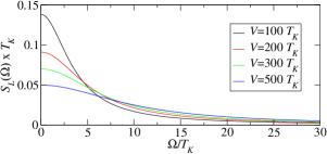
Figure 8: (color online) Longitudinal correlation function $S_{L}(\Omega)\equiv S_{S^{z}S^{z}}(\Omega)$ in the symmetric Kondo model ($r=1$) for various values of the applied voltage $V$.

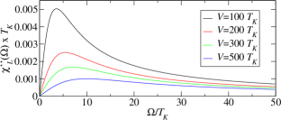
Figure 9: (color online) Imaginary part of the longitudinal susceptibility $\chi_{L}^{\prime\prime}(\Omega)\equiv\chi_{S^{z}S^{z}}^{\prime\prime}(\Omega)$ in the symmetric Kondo model ($r=1$) for various values of the applied voltage $V$.

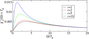
Figure 10: (color online) Imaginary part of the longitudinal susceptibility $\chi_{S^{z}S^{z}}^{\prime\prime}(\Omega)$ for $V=100\,T_{K}$ and various values of the asymmetry ratio $r=J_{L}/J_{R}$.

Let us further study the behavior of the correlation functions analytically. For small values of the frequency $S_{S^{z}S^{z}}(\Omega)$ has the Lorentzian form

$$S_{S^{z}S^{z}}(\Omega)=\frac{1}{2}\frac{\tilde{\Gamma}_{1}}{\Omega^{2}+\tilde{\Gamma}_{1}^{2}}\stackrel{{\scriptstyle\Omega\rightarrow 0}}{{\longrightarrow}}\frac{1}{2\tilde{\Gamma}_{1}}=\frac{1}{2\pi\,J_{R}J_{L}\,V},$$ (214)

where we have used $Re\,\Gamma^{a}(0)=\tilde{\Gamma}_{1}$. This result for the small-frequency regime agrees with conclusions drawn from a mapping of the spin correlators to the one-particle Green’s function of Majorana fermions Mao-03 ; ShnirmanMakhlin03 . On the other hand, in the limit of large frequencies we find

$$S_{S^{z}S^{z}}(\Omega)=\frac{\pi}{4}\frac{(J_{R}+J_{L})^{2}}{\Omega}\propto\frac{1}{\Omega}\frac{1}{\ln^{2}\frac{\Omega}{T_{K}}}$$ (215)

in agreement with the flow-equation method FritschKehrein09ap ; Kehreinbook . We note that the $J^{\prime}s$ appearing in the correlation function (212) have their origin in the resolvent $1/(\Omega-L_{S}^{eff}(\Omega))$, hence the external frequency $\Omega$ serves as a cut-off parameter in $\Lambda_{c}$. This results in the logarithmic corrections at large frequencies.

The susceptibility in the limiting regimes reads

$$\chi_{S^{z}S^{z}}^{\prime\prime}(\Omega) = \frac{(1+r)^{2}}{4\pi\,r\,J_{R}J_{L}\,V^{2}}\,\Omega,\quad\Omega\rightarrow 0,\quad$$ (216)

$$\chi_{S^{z}S^{z}}^{\prime\prime}(\Omega) = S_{S^{z}S^{z}}(\Omega),\quad\Omega\rightarrow\infty.$$ (217)

The first result shows a dependence of the gradient at small $\Omega$ on the asymmetry ratio $r=J_{L}/J_{R}$, while the second result indicates the revival of the fluctuation-dissipation theorem (37) for $\Omega\gg V$. We note that the derivation of (217) relies on the fact that the coupling constants $J_{c}$ appearing in the kernel $\Sigma_{S^{z}}^{-}$ are cut-off by the external frequency $\Omega$, as it was discussed at the end of Sec. VI. Furthermore, the susceptibility $\chi_{S^{z}S^{z}}^{\prime\prime}(\Omega)$ has a maximum at $\Omega\approx\tilde{\Gamma}_{1}$, where it takes the value

$$\chi_{S^{z}S^{z}}^{\prime\prime}(\Omega\approx\tilde{\Gamma}_{1})\approx\frac{(1+r)^{2}}{8rV}.$$ (218)

This behavior was also deduced using the flow-equation method Kehreinbook .

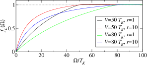
Figure 11: (color online) Longitudinal fluctuation-dissipation ratio $f_{L}(\Omega)$ for various values of the asymmetry $r$ and applied voltage $V$. In order to get a smooth behavior at $\Omega\approx V$ we have kept the $\arctan$ in the definition of $\mathcal{H}_{i}$ in this region. The dotted line is a guide to the eye.

In order to investigate the revival of the fluctuation-dissipation theorem we introduce the longitudinal fluctuation-dissipation ratio Mao-03 ; ShnirmanMakhlin03 ; MitraMillis05

$$f_{L}(\Omega)=\frac{\chi_{S^{z}S^{z}}^{\prime\prime}(\Omega)}{S_{S^{z}S^{z}}(\Omega)},$$ (219)

which is in equilibrium simply given by $f_{L}(\Omega)=\tanh\frac{\Omega}{2T}\rightarrow\text{sgn}(\Omega)\,$ ($T\rightarrow 0$). Using our results (212) and (213) we obtain

$$f_{L}(\Omega)=\frac{\pi}{2}\frac{(J_{R}+J_{L})^{2}}{Re\,\Gamma^{a}(\Omega)}\,\Omega,$$ (220)

which is plotted in Fig. 11. We find $f_{L}(\Omega>V)=1$, i.e. the equilibrium result, whereas for small frequencies we get

$$f_{L}(\Omega\ll V)=\frac{(1+r)^{2}}{2r}\,\frac{\Omega}{V},$$ (221)

in agreement with Refs. Mao-03, ; ShnirmanMakhlin03, . We note that $f_{L}(\Omega<V)$ increases with increasing asymmetry $r$ as the coupling of the voltage to the dot becomes less effective.

VII.2 Longitudinal correlation functions in a weak magnetic field ($\boldsymbol{V>\tilde{h}}$)

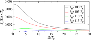
Figure 12: (color online) Longitudinal correlation function $S_{S^{z}S^{z}}(\Omega)$ in the symmetric Kondo model ($r=1$) for $V=100\,T_{K}$ and various values of the applied magnetic field $h_{0}$. For $h_{0}=115\,T_{K}$ we already have $V<\tilde{h}$, which implies $S_{S^{z}S^{z}}(\Omega<\tilde{h}-V)=0$ in order $J_{c}^{2}$ (see Sec. VII.3).

In the presence of an external magnetic field the stationary reduced density matrix is given by $\rho_{\uparrow\uparrow}=1+M$, $\rho_{\downarrow\downarrow}=1-M$, $\rho_{\uparrow\downarrow}=\rho_{\downarrow\uparrow}=0$, with the magnetization in leading order SchoellerReininghaus09 (see also Refs. ParcolletHooley02, ; Rosch-03prl, ; Paaske-04prb1, ; Rosch-05, )

$$M=-\frac{1}{2}\frac{\Gamma^{3z}(0)}{\Gamma^{a}(0)}=-\frac{1}{2}\frac{(1+r)^{2}\tilde{h}}{(1+r^{2})\tilde{h}+2rV}.$$ (222)

To evaluate the correlation function we now use

$$\begin{split}&\mbox{Tr}_{S}\Bigl{[}\Sigma_{S^{z}}(\Omega)\,P_{i}(\Omega)\,\Sigma_{S^{z}}^{+}(\Omega,\text{i}0+)\,\rho_{S}^{st}\Bigr{]}\\ &\qquad\qquad=\left\{\begin{array}[]{ll}M\frac{\Gamma^{3z}(\Omega)}{\Gamma^{a}(\Omega)},&i=0,\\ -\frac{1}{2}-M\frac{\Gamma^{3z}(\Omega)}{\Gamma^{a}(\Omega)},&i=1,\\ 0,&i=\pm,\end{array}\right.\end{split}$$ (223)

where the term $\Gamma_{S^{z}}^{+c}(\Omega)\,L^{c}$ again does not contribute. From this a straightforward calculation using (211) yields the correlation function up to $O(J_{c}^{2})$

$$S_{S^{z}S^{z}}(\Omega)=\frac{1}{2}\frac{Re\,\Gamma^{a}(\Omega)+2M\,\Gamma^{3z}(\Omega)}{\Omega^{2}+Re\,\Gamma^{a}(\Omega)^{2}},$$ (224)

where the zero-frequency $\delta$-peak does not appear because of our definition (25). The suppression of the correlation function by the finite magnetic field is shown in Fig. 12, which agrees very well with similar plots obtained using the flow-equation method FritschKehrein09 . In the zero-frequency limit we find

$$S_{S^{z}S^{z}}(\Omega\rightarrow 0)=\frac{4r^{2}}{\pi J_{R}J_{L}}\frac{(1+r+r^{2})\tilde{h}+rV}{((1+r^{2})\tilde{h}+2rV)^{3}}(V-\tilde{h}),$$ (225)

while the leading term $\propto 1/\Omega$ in the large frequency regime is given by (215) (including the logarithmic corrections in the coupling constants). Furthermore we observe a weak feature at $\Omega=V-\tilde{h}$ which has for $\tilde{\Gamma}_{2}\ll V-\tilde{h}\ll\tilde{h}$ the line shape

$$S_{S^{z}S^{z}}(\Omega)\! \approx \!\frac{\pi J_{R}J_{L}}{8\Omega^{2}}\biggl{[}\bigl{(}2+r+2r^{2}+4M(1+r)^{2}\bigr{)}\frac{\tilde{h}}{r}+3V$$ (226)

$$+\Omega+\frac{2}{\pi}(\Omega-V+\tilde{h})\arctan\frac{\Omega-V+\tilde{h}}{\tilde{\Gamma}_{2}}\biggr{]}.\quad$$

Similar features appear at $\Omega=\tilde{h},V+\tilde{h}$.

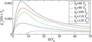
Figure 13: (color online) Imaginary part of the longitudinal susceptibility $\chi_{S^{z}S^{z}}^{\prime\prime}(\Omega)$ in the symmetric Kondo model ($r=1$) for $V=100\,T_{K}$ and various values of the applied magnetic field $h_{0}$. For $h_{0}=120\,T_{K}$ we have $V<\tilde{h}$, which implies $\chi_{S^{z}S^{z}}(\Omega<\tilde{h}-V)=0$ in order $J_{c}^{2}$ (see Sec. VII.3).

For the calculation of the susceptibility we need

$$\begin{split}&\mbox{Tr}_{S}\Bigl{[}\Sigma_{S^{z}}(\Omega)\,P_{i}(\Omega)\,\Sigma_{S^{z}}^{-}(\Omega,\text{i}0+)\,\rho_{S}^{st}\Bigr{]}\\ &\qquad\qquad=\left[\frac{\text{i}}{2}\,\Gamma_{S^{z}}^{-,3z}(\Omega)+\text{i}\,M\,\Gamma_{S^{z}}^{-,a}(\Omega)\right]\delta_{i1},\end{split}$$ (227)

which directly yields

$$\chi_{S^{z}S^{z}}^{\prime}(\Omega) = \frac{1}{\Omega^{2}+Re\,\Gamma^{a}(\Omega)^{2}}\biggl{[}-M\,\Omega\,Im\,\Gamma_{S^{z}}^{-,a}(\Omega)$$ (228)

$$+\left(\frac{\pi}{4}(J_{R}+J_{L})^{2}+M\,Re\,\Gamma_{S^{z}}^{-,a}(\Omega)\right)Re\,\Gamma^{a}(\Omega)\biggr{]},\quad$$

$$\chi_{S^{z}S^{z}}^{\prime\prime}(\Omega) = \left[\frac{\pi}{4}(J_{R}+J_{L})^{2}+M\,Re\,\Gamma_{S^{z}}^{-,a}(\Omega)\right]$$ (229)

$$\qquad\times\frac{\Omega}{\Omega^{2}+Re\,\Gamma^{a}(\Omega)^{2}}.$$

In (228) we have kept the terms in the second line, which are of $O(J_{c}^{4})$, as due to $\Omega\,Im\,\Gamma_{S^{z}}^{-,a}(\Omega)\rightarrow 0$ ($\Omega\rightarrow 0$) they become dominant in the small-frequency limit. For larger frequencies these terms have to be neglected. Thus the static susceptibility (34) is given in leading order by

$$\chi_{S^{z}S^{z}}=-\frac{r(1+r)^{2}V}{((1+r^{2})\tilde{h}+2rV)^{2}}$$ (230)

in agreement with the literature ParcolletHooley02 ; Rosch-03prl ; Paaske-04prb1 ; Rosch-05 ; SchoellerReininghaus09 . For larger frequencies the real part of the susceptibility possesses logarithmic features at $\Omega=\tilde{h},V\pm\tilde{h}$ due to the term $Im\,\Gamma_{S^{z}}^{-,a}(\Omega)$. For example,

$$\begin{split}&\chi_{S^{z}S^{z}}^{\prime}(\Omega\approx\tilde{h})\approx\\ &\quad-M(J_{R}+J_{L})^{2}\frac{\Omega-\tilde{h}}{2\Omega^{2}}\ln\frac{\Lambda_{c}}{\sqrt{(\Omega-\tilde{h})^{2}+\tilde{\Gamma}_{2}^{2}}}+\ldots,\end{split}$$ (231)

where the terms represented by the dots do not contain any logarithmic features at $\Omega=\tilde{h}$. The imaginary part of the susceptibility is plotted in Fig. 13. It has a finite gradient at $\Omega=0$ given by

$$\chi_{S^{z}S^{z}}^{\prime\prime}(\Omega\rightarrow 0)=\frac{2}{\pi}\frac{r^{2}(1+r)^{2}V}{((1+r^{2})\tilde{h}+2rV)^{3}}\frac{\Omega}{J_{R}J_{L}}$$ (232)

as well as a maximum at $\Omega\approx\tilde{\Gamma}_{1}$, where it takes the value

$$\chi_{S^{z}S^{z}}^{\prime\prime}(\Omega\approx\tilde{\Gamma}_{1})\approx\frac{r}{2}\frac{(1+r)^{2}V}{((1+r^{2})\tilde{h}+2rV)^{2}}=-\frac{1}{2}\chi_{S^{z}S^{z}}.$$ (233)

In the large-frequency limit $\chi_{S^{z}S^{z}}^{\prime\prime}(\Omega\gg V,\tilde{h})$ coincides with the correlation function (215). Furthermore, the imaginary part of the susceptibility has features at $\Omega=\tilde{h},V\pm\tilde{h}$ which have their origin in the function $Im\,\mathcal{H}_{2}$ contained in $Re\,\Gamma_{S^{z}}^{-,a}(\Omega)$ and hence have a line shape similar to (226).

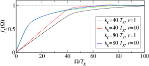
Figure 14: (color online) Fluctuation-dissipation ratio $f_{L}(\Omega)$ for $V=80\,T_{K}$ and different values of the asymmetry $r$ and magnetic field $h_{0}$. In order to get a smooth behavior at $\Omega\approx V-\tilde{h}$ we have kept the $\arctan$ in the definition of $\mathcal{H}_{i}$. For $V<\tilde{h}$ the fluctuation-dissipation ratio is independently of $\Omega$ given by $f_{L}(\Omega)=1$. The dotted line is a guide to the eye.

The fluctuation-dissipation ratio $f_{L}(\Omega)$ defined in (219) reads in the presence of a magnetic field

$$f_{L}(\Omega)=\frac{\frac{\pi}{2}(J_{R}+J_{L})^{2}\Omega+2M\,Re\,\Gamma_{S^{z}}^{-,a}(\Omega)\,\Omega}{Re\,\Gamma^{a}(\Omega)+\pi(J_{R}+J_{L})^{2}M\tilde{h}},$$ (234)

which is plotted in Fig. 14. Larger values of the magnetic field push the system closer to its equilibrium behavior, as only those lead electrons in the energy interval $V-\tilde{h}$ can couple to the dot and thus induce the non-equilibrium behavior. We note, however, that the equilibrium result $f_{L}(\Omega)=1$ is only reached for $\Omega>V+\tilde{h}$. Furthermore, increasing the asymmetry $r$ drives the system towards the equilibrium situation as the coupling of the voltage to the dot becomes less effective. This effect is suppressed by increasing the magnetic field as overall less electrons couple to the dot. For small frequencies we obtain

$$f_{L}(\Omega\rightarrow 0)=\frac{1}{2}\frac{(1+r)^{2}V}{(1+r+r^{2})\tilde{h}+rV}\frac{\Omega}{V-\tilde{h}}.$$ (235)

VII.3 Longitudinal correlation functions in a strong magnetic field ($\boldsymbol{V<\tilde{h}}$)

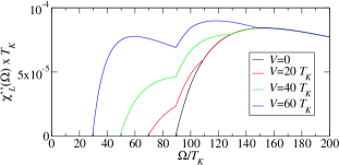
Figure 15: (color online) Imaginary part of the longitudinal susceptibility $\chi_{S^{z}S^{z}}^{\prime\prime}(\Omega)$ in the symmetric Kondo model ($r=1$) for $h_{0}=100\,T_{K}$ and various values of the applied voltage $V$. The correlation function is given by $S_{S^{z}S^{z}}^{\prime\prime}(\Omega)=\chi_{S^{z}S^{z}}(\Omega)$. For $\Omega<\tilde{h}-V$ the susceptibility vanishes in order $J_{c}^{2}$. The line shape close to $\Omega=\tilde{h}$ is given by (236).

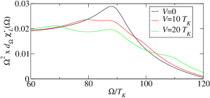
Figure 16: (color online) Derivative of the real part of the longitudinal susceptibility $\Omega^{2}\,\frac{d}{d\Omega}\chi_{S^{z}S^{z}}^{\prime}(\Omega)$ in the symmetric Kondo model ($r=1$) for $h_{0}=100\,T_{K}$ and various values of the applied voltage $V$. We observe characteristic logarithmic features at $\Omega=\tilde{h},\tilde{h}\pm V$.

In the case of a strong magnetic field, $V<\tilde{h}$, the correlation functions up to quadratic order in the coupling are still given by (224), (228) and (229), respectively, where the magnetization is simply $M=-1/2$. One can easily show using $Im\,\mathcal{H}_{2}(\Omega)=\frac{\pi}{2}|\Omega|$ that $\chi_{S^{z}S^{z}}^{\prime\prime}(\Omega>0)=S_{S^{z}S^{z}}(\Omega>0)$, which implies the equilibrium result $f_{L}(\Omega>0)=1$. Furthermore, the correlation function vanishes identically in order $J_{c}^{2}$ for $\Omega<\tilde{h}-V$. Physically the Kondo spin is in its ground state $\left|\downarrow\right\rangle$ and the energy difference to the state $\left|\uparrow\right\rangle$ due to the external magnetic field is given by $\tilde{h}$. Hence one has to apply at least the frequency $\tilde{h}-V$ to obtain any response from the spin, where the energy $V$ is provided by the applied voltage.

This has to be contrasted with the result for the susceptibility in the equilibrium Kondo model derived by Garst et al. Garst-05 . They used a relation between the inelastic electron scattering and the correlation function to show that the susceptibility in equilibrium has the small-frequency behavior $\chi_{S^{z}S^{z}}^{\prime\prime}(\Omega)\propto J_{c}^{4}\,\Omega$, i.e. it is non-zero for $\Omega<\tilde{h}$. This linear behavior was also observed by Costi and Kieffer CostiKieffer96 as well as Hewson Hewson06 using a numerical renormalization group calculation. In analogy, we expect the non-equilibrium correlation functions to be nonzero for $\Omega<\tilde{h}-V$ in higher order in $J_{c}$. The consistent calculation of terms $\sim J_{c}^{4}$ in the real-time RG procedure applied here would involve, however, 5-loop diagrams and is hence beyond the scope of this work.

The correlation function in the regime $V<\tilde{h}$ is plotted in Fig. 15. We find excellent agreement with numerical results recently obtained by Fritsch and Kehrein using the flow-equation method FritschKehrein09 . In particular, we observe a splitting of the sharp edge at $\Omega=\tilde{h}$ due to the applied voltage, which leads to characteristic features at $\Omega=\tilde{h},\tilde{h}\pm V$. Using our result (224) we can derive analytic expressions for the line shape close to these frequencies. For example, at $\Omega\approx\tilde{h}$ we find

$$\chi_{S^{z}S^{z}}^{\prime\prime}(\Omega) \approx \frac{\pi J_{R}J_{L}\,V}{4\Omega^{2}}+\frac{\pi}{8}(J_{R}+J_{L})^{2}\frac{\Omega-\tilde{h}}{\Omega^{2}}$$ (236)

$$+\frac{1}{4}(J_{R}^{2}+J_{L}^{2})\frac{\Omega-\tilde{h}}{\Omega^{2}}\,\arctan\frac{\Omega-\tilde{h}}{\tilde{\Gamma}_{2}}.$$

The first term shows that the gradient of $\chi_{S^{z}S^{z}}^{\prime\prime}(\Omega)$ will become negative for $\Omega<\tilde{h}$ if the applied voltage is large enough, i.e. $V>\tilde{h}/2$. In the vicinity of $\Omega=\tilde{h}\pm V$ the correlation function shows similar kink-like behavior (236). The physical origin of these kinks lies in the fact that at each of the energies $\Omega=\tilde{h},\tilde{h}\pm V$ a new process sets in, which involves a spin-flip on the dot costing the Zeeman energy $\tilde{h}$ as well as the virtual hopping of an electron on and off the dot gaining or costing the energy $-V$, $0$, or $V$, respectively. The real part $\chi_{S^{z}S^{z}}^{\prime}(\Omega)$ of the susceptibility shows logarihmic features (231) at $\Omega=\tilde{h},\tilde{h}\pm V$ as is shown in Fig. 16.We stress that the splitting of the sharp edge at $\Omega=\tilde{h}$ is a true non-equilibrium effect.

VIII Transverse correlation functions

Finally let us discuss the transverse correlation functions in the presence of a magnetic field. We note that by virtue of (36) we can restrict ourselves to the $S^{-}S^{+}$-correlations. The corresponding kernels up to second order in $J_{c}$ were calculated in (156), (157), (159), (160), (163)–(166) as well as (200). We will first discuss the susceptibility and present the results for the correlation function afterwards.

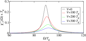
Figure 17: (color online) Imaginary part of the transverse susceptibility $\chi_{T}^{\prime\prime}(\Omega)\equiv\chi_{S^{-}S^{+}}^{\prime\prime}(\Omega)$ in the symmetric Kondo model ($r=1$) for $h_{0}=100\,T_{K}$ and various values of the applied voltage $V$.

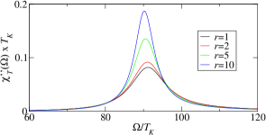
Figure 18: (color online) Imaginary part of the transverse susceptibility $\chi_{S^{-}S^{+}}^{\prime\prime}(\Omega)$ for $V=200\,T_{K}$, $h_{0}=100\,T_{K}$, and various values of the asymmetry ratio $r=J_{L}/J_{R}$. The result is invariant under $r\rightarrow 1/r$.

In order to derive the susceptibility we start with the parametrization

$$\Sigma_{S^{+}}^{-}(\Omega,\text{i}0+)=\Gamma_{S^{+}}^{-,2}\,L^{2}_{+}+\Gamma_{S^{+}}^{-,3}\,L^{3}_{+}+\Gamma_{S^{+}}^{-,5}(\Omega)\,L^{5}_{+},$$ (237)

where for example $\Gamma_{S^{+}}^{-,2}=-2\text{i}-\text{i}\,\mathrm{tr}J_{c}+\text{i}\frac{3}{4}\mathrm{tr}J_{c}^{2}=-2\text{i}-\text{i}(J_{R}+J_{L})+\text{i}\frac{3}{4}(J_{R}+J_{L})^{2}$. Note that we already indicated that the explicit frequency dependence in order $J_{c}^{2}$ appears in $\Gamma_{S^{+}}^{-,5}$ exclusively. (There is of course an implicit frequency dependence of $\Gamma_{S^{+}}^{-,2}$ and $\Gamma_{S^{+}}^{-,3}$ through $J_{c}$.) Now using

$$\mbox{Tr}_{S}\Bigl{[}\Sigma_{S^{-}}(\Omega)\,P_{i}(\Omega)\,\Sigma_{S^{+}}^{-}(\Omega,\text{i}0+)\,\rho_{S}^{st}\Bigr{]}$$

$$\qquad=\text{i}\left(\Gamma_{S^{+}}^{-,3}+\bigl{(}\Gamma_{S^{+}}^{-,2}+2\Gamma_{S^{+}}^{-,5}(\Omega)\bigr{)}M\right)\delta_{i+}\qquad$$ (238)

we obtain

$$\chi_{S^{-}S^{+}}(\Omega)=\text{i}\,\frac{\Gamma_{S^{+}}^{-,3}+\bigl{(}\Gamma_{S^{+}}^{-,2}+2\Gamma_{S^{+}}^{-,5}(\Omega)\bigr{)}M}{\Omega-h(\Omega)+\text{i}\Gamma_{2}(\Omega)},$$ (239)

where we have introduced the short-hand notation $\Gamma_{2}(\Omega)=\Gamma^{a}(\Omega)+\Gamma^{c}(\Omega)$. For $h_{0}=0$ we find $\chi_{S^{-}S^{+}}(\Omega)=2\chi_{S^{z}S^{z}}(\Omega)$. The transverse susceptibility has a peak at the solution of

$$\Omega-Re\,h(\Omega)-Im\,\Gamma_{2}(\Omega)=0,$$ (240)

which is up to first order solved by

$$\Omega=\left(1-\frac{1}{2}(J_{R}+J_{L})\right)h_{0}=\tilde{h}.$$ (241)

In a finite magnetic field the spin on the dot will be in its ground state $\left|\downarrow\right\rangle$. The energy difference to the excited state $\left|\uparrow\right\rangle$ is given by $\tilde{h}$, leading to an enhanced response of the system at this frequency. At the peak the imaginary part of the susceptibility takes the value

$$\chi_{S^{-}S^{+}}^{\prime\prime}(\Omega\approx\tilde{h})\approx-\frac{2M}{\tilde{\Gamma}_{2}},$$ (242)

as is shown in Figs. 17 and 18. The peak is suppressed by increasing the voltage, since this reduces the probability for the Kondo spin to be in its ground state. On the other hand, for a fixed value of the voltage the peak increases with increasing asymmetry ratio as the coupling of the voltage to the dot becomes less effective. The width of the peak is up to order $J_{c}^{2}$ given by

$$Re\,\Gamma_{2}(\tilde{h})-Im\,h(\tilde{h})=\tilde{\Gamma}_{2}$$ (243)

with the limiting cases

$$V\ll\tilde{h}: \frac{\pi}{4}(J_{R}+J_{L})^{2}\,h_{0},$$ (244)

$$\tilde{h}\ll V: \pi J_{R}J_{L}V.$$ (245)

In the equilibrium limit, $V=0$, this corresponds to the result obtained in Ref. GoetzeWoelfle71, . The real part of the transverse susceptibility possesses logarithmic features similar to (231) at $\Omega=\tilde{h},\tilde{h}\pm V$.

Using a pseudo-fermion representation of the Kondo spin together with non-equilibrium perturbation theory Paaske et al. Paaske-04prb2 previously obtained the transverse susceptibility. In order to compare these results to (239) we first make the approximations $h(\Omega)\rightarrow h_{0}$ and $\Gamma_{2}(\Omega)\rightarrow\tilde{\Gamma}_{2}$. In the limit $h_{0}\rightarrow 0$ we then obtain using $\Gamma_{S^{+}}^{-,3}=\frac{\pi}{2}(J_{R}+J_{L})^{2}$

$$\chi_{S^{-}S^{+}}(\Omega)\approx\text{i}\frac{\pi}{2}\frac{(J_{R}+J_{L})^{2}}{\Omega+\text{i}\tilde{\Gamma}_{2}}.$$ (246)

In the regime $h_{0}\gg\tilde{\Gamma}_{2}$ we have $M=O(J_{c}^{0})$, thus we can neglect $\Gamma_{S^{+}}^{-,3}$ as well as $\Gamma_{S^{+}}^{-,5}$ in the numerator in (239), which results in

$$\chi_{S^{-}S^{+}}(\Omega)\approx\frac{2M}{\Omega-h_{0}+\text{i}\tilde{\Gamma}_{2}}.$$ (247)

These approximations agree with the results obtained in Ref. Paaske-04prb2, (we have to replace $h_{0}\rightarrow-B$ due to a different sign in the definition of the bare dot Hamiltonian $H_{S}$). Furthermore, in the regime $\Omega,h_{0}<V$ we can use

$$\Gamma_{S^{+}}^{-,3}+\bigl{(}\Gamma_{S^{+}}^{-,2}+2\Gamma_{S^{+}}^{-,5}(\Omega)\bigr{)}\,M\rightarrow-2\frac{M}{h_{0}}\tilde{\Gamma}_{2}-2\text{i}\,M,$$ (248)

where we have replaced $Im\,\mathcal{H}_{i}(\Omega)\rightarrow\frac{\pi}{2}|\Omega|$ in the real part of $\Gamma_{S^{+}}^{-,5}$, to obtain

$$\chi_{S^{-}S^{+}}(\Omega)\approx\frac{2M}{h_{0}}\frac{h_{0}-\text{i}\tilde{\Gamma}_{2}}{\Omega-h_{0}+\text{i}\tilde{\Gamma}_{2}}.$$ (249)

This confirms a conjecture by Paaske et al. Paaske-04prb2 . We would like to stress, however, that our result (239) goes beyond the approximation (249).

In analogy to the susceptibility one finds for the correlation function

$$\begin{split}&S_{S^{-}S^{+}}(\Omega)=\\ &\frac{Re\,\Gamma_{2}(\Omega)-Im\,h(\Omega)-\frac{\pi}{2}M(J_{R}+J_{L})^{2}(\Omega-h_{0})}{(\Omega\!-\!Re\,h(\Omega)\!-\!Im\,\Gamma_{2}(\Omega))^{2}\!+\!(Re\,\Gamma_{2}(\Omega)\!-\!Im\,h(\Omega))^{2}},\end{split}$$ (250)

where we have neglected all terms of order $J_{c}^{3}$ in the numerator. This allows the calculation of the transverse fluctuation-dissipation ratio

$$f_{T}(\Omega)=\frac{\chi_{S^{-}S^{+}}^{\prime\prime}(\Omega)}{S_{S^{-}S^{+}}(\Omega)}$$ (251)

which is plotted in Fig. 19. For negative frequencies $\Omega<-V$ the fluctuation-dissipation ratio takes the value $f_{T}(\Omega)=-1$, whereas for frequencies $\Omega>V$ we find $f_{T}(\Omega)=1$, thus recovering the equilibrium situation in these limits. As for the longitudinal fluctuation-dissipation ration we observe that increasing the magnetic field or the asymmetry ratio $r$ drives the system towards the equilibrium situation.

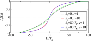
Figure 19: (color online) Transverse fluctuation-dissipation ratio $f_{T}(\Omega)$ for $V=80\,T_{K}$ and various values of the asymmetry ration $r$ and the applied magnetic field $h_{0}$. The plot shows good agreement with similar results obtained in Ref. MitraMillis05, . The dotted line is a guide to the eye.

IX Conclusions

In this article we have generalized the real-time renormalization group method in frequency space to allow the calculation of dynamical correlation functions of arbitrary dot operators in systems describing spin and/or orbital fluctuations. We applied this to the two-lead Kondo model in a magnetic field, where we calcualted the longitudinal and transverse spin-spin correlation and response functions up to second order in the exchange coupling. We wish to stress that within this formalism the Kondo spin is directly represented by matrices in Liouville space, hence there is no need to apply a pseudo-fermion representation. Specifically, we derived the two-loop RG equations for the dot operators and solved them analytically up to order $J_{c}^{2}$ in the weak-coupling regime. Here $J_{c}$ denotes the effective coupling at the energy scale $\Lambda_{c}=\max\{V,h_{0}\}$ which has to satisfy $\Lambda_{c}\gg T_{K}$. Our results show several features attributed to the non-equilibrium situation, e.g. the splitting of the edge at $\Omega=\tilde{h}$ of the longitudinal correlation function in a strong magnetic field or the suppression of the peak in the transverse susceptibility by a finite applied voltage. Furthermore, we find very good agreement with results for the longitudinal correlation function recently obtained by Fritsch and Kehrein using the flow-equation method FritschKehrein09ap ; FritschKehrein09 . A particular advantage of our approach is the possibility to obtain analytic expressions for all correlation functions in the weak coupling limit.

We have calculated the spin-spin correlation functions for the nonequilibrium Kondo model in the weak coupling regime $\Lambda_{c}\gg T_{K}$. The regime of strong coupling, $\Lambda_{c}<T_{K}$, is still an open problem. In this case, the exchange couplings $J_{c}$ become of order $O(1)$ and a controlled truncation of the RG equations is no longer possible. Within the present RTRG-FS method it was shown in Ref. Schoeller09, that the relaxation/dephasing rates saturate to the Kondo temperature in the strong coupling regime. As an effect the coupling constants do not diverge as in poor man scaling methods but remain finite. However, the numerical solution of the RG equations in lowest order showed an instability against an exponentionally small change in the initial condition for the relaxation/dephasing rates. Although it was possible to find excellent agreement for the temperature dependence of the linear conductance with NRG calculations, it was necessary to fine tune the initial condition for the rates. Therefore, up to now, it is not yet clear whether a controlled solution of the strong coupling regime is possible by using RTRG-FS.

The nonequilibrium Kondo model describes the spin fluctuation (or Coulomb blockade) regime of the more general nonequilibrium Anderson impurity model (for a systematic derivation of the Kondo model from the Anderson model using a Schrieffer-Wolff transformation, see e.g. Ref. Korb-07, ). In this model the single-particle spectral function is of most interest, which has recently been studied within NRG in a scattering wave basis Anders08prl ; Anders08 . The present RTRG-FS method can also be applied to this model but, as explained in detail in Ref. Schoeller09, , in the charge fluctuation regime it is not yet clear whether a well-defined weak coupling regime exists at zero temperature. At resonance (i.e. when the renormalized single-particle level is identical to one of the chemical potentials of the leads) there is no energy scale except the broadening of the level itself and the expansion parameter is of order $O(1)$. Nevertheless the results obtained in Ref. SchoellerKoenig00, (using a previous version of the real-time RG method) after an a priori uncontrolled truncation of the RG equations were in excellent agreement with the Bethe Ansatz solution TsvelikWiegmann83 for the equilibrium occupation of the local level. These and related topics are of high interest and will be the subject of forthcoming research.

Appendix A Derivation of (32) and (33)

Obviously the time-dependent correlation function can be written as

$$S_{AB}(t)=\frac{1}{2}\Bigl{\langle}\left[A(t)_{\mathrm{H}},B(0)_{\mathrm{H}}\right]_{+}\Bigr{\rangle}_{st}-\bigl{\langle}A\bigr{\rangle}_{st}\bigl{\langle}B\bigr{\rangle}_{st}.$$ (252)

Now, applying the time-translational invariance

$$\Bigl{\langle}A(t_{1})_{\mathrm{H}}\,B(t_{2})_{\mathrm{H}}\Bigr{\rangle}_{st}=\Bigl{\langle}A(t_{1}+t)_{\mathrm{H}}\,B(t_{2}+t)_{\mathrm{H}}\Bigr{\rangle}_{st}$$ (253)

for all $t,t_{1},t_{2}$ fixed and finite as well as the relation

$$\Bigl{\langle}\left[A(0)_{\mathrm{H}},B(t)_{\mathrm{H}}\right]_{\pm}\Bigr{\rangle}_{st}^{*}=\Bigl{\langle}\left[A(t)_{\mathrm{H}},B(0)_{\mathrm{H}}\right]_{\pm}\Bigr{\rangle}_{st},$$ (254)

which can be verified by a straightforward calculation using $B=A^{\dagger}$, we obtain (32). In the same way (253) can be used to derive the relation $\chi_{AB}(\Omega)=\text{i}\,C_{AB}^{-}(\Omega)$.

Appendix B Derivation of $\boldsymbol{\mathcal{B}_{\pm,11^{\prime}}^{(2)}}$

In this appendix we will calculate the vertex $\mathcal{B}_{\pm,11^{\prime}}^{(2)}$. Starting from (102) we first take the zero-temperature limit. Furthermore, we can expand the resolvents up to $O(J)$ asSchoellerReininghaus09

$$\!\!\!\!\!\!\!\!\!\!\!\!\!\!\!\!\!\Pi(E,\omega)=\frac{1}{E+\text{i}\omega-L_{S}^{(0)}-L_{S}^{(1)}-(E+\text{i}\omega)Z^{(1)}}$$

$$\!\!\!\!\!\!\!\!\!\!\!\!\!=\left(1-\frac{Z^{(1)}}{2}\right)\frac{1}{E+\text{i}\omega-L_{S}^{(0)}-\tilde{L}_{S}^{(1)}}\left(1-\frac{Z^{(1)}}{2}\right)$$ (255)

with

$$\tilde{L}_{S}^{(1)}=L_{S}^{(1)}-\frac{1}{2}\left[Z^{(1)},L_{S}^{(0)}\right]_{+}.$$ (256)

Using this we obtain together with the expansion $\mathcal{B}_{\pm}=\mathcal{B}_{\pm}^{(0)}+\mathcal{B}_{\pm}^{(1)}$ in (102)

$$\frac{d}{d\Lambda}\mathcal{B}_{\pm,11^{\prime}}(\Omega,\delta,\xi,\xi^{\prime};\omega_{1},\omega_{1^{\prime}})=\text{i}\,\bar{G}_{12}\left(1-\frac{Z^{(1)}}{2}\right)\frac{1}{\Omega_{12}+\text{i}\delta+\text{i}\Lambda+\text{i}\omega_{1}-L_{S}^{(0)}-\tilde{L}_{S}^{(1)}}$$

$$\qquad\times\left(\mathcal{B}_{\pm}^{(0)}+\mathcal{B}_{\pm}^{(1)}-\frac{1}{2}\left[Z^{(1)},\mathcal{B}_{\pm}^{(0)}\right]_{+}\right)\frac{1}{\xi_{12}+\text{i}\xi^{\prime}+\text{i}\Lambda+\text{i}\omega_{1}-L_{S}^{(0)}-\tilde{L}_{S}^{(1)}}\left(1-\frac{Z^{(1)}}{2}\right)\bar{G}_{\bar{2}1^{\prime}}-(1\leftrightarrow 1^{\prime}),$$ (257)

where we have omitted the arguments of the vertices $\bar{G}$ for simplicity. Using

$$\left[L_{S}^{(0)}+\tilde{L}_{S}^{(1)},\mathcal{B}_{\pm}^{(0)}\right]_{-}=\tilde{\kappa}\,\mathcal{B}_{\pm}^{(0)},\quad\left[L_{S}^{(0)}+\tilde{L}_{S}^{(1)},\mathcal{B}_{\pm}^{(1)}\right]_{-}=\tilde{\kappa}\,\mathcal{B}_{\pm}^{(1)},\quad\left[L_{S}^{(0)}+\tilde{L}_{S}^{(1)},\left[Z^{(1)},\mathcal{B}_{\pm}^{(0)}\right]_{+}\right]_{-}=\tilde{\kappa}\,\left[Z^{(1)},\mathcal{B}_{\pm}^{(0)}\right]_{+},$$ (258)

with $\tilde{\kappa}=\pm h_{0}\mp\frac{h_{0}}{2}\,\mathrm{tr}\,J$ for $B=S^{\pm}$ and $\tilde{\kappa}=0$ for $B=S^{z}$ (see Sec. VI) we obtain after a partial fraction expansion

$$\frac{d}{d\Lambda}\mathcal{B}_{\pm,11^{\prime}}(\Omega,\delta,\xi,\xi^{\prime};\omega_{1},\omega_{1^{\prime}})=-\frac{\text{i}}{\Omega-\xi-\tilde{\kappa}+\text{i}(\delta-\xi^{\prime})}\bar{G}_{12}\left(1-\frac{Z^{(1)}}{2}\right)\left(\mathcal{B}_{\pm}^{(0)}+\mathcal{B}_{\pm}^{(1)}-\frac{1}{2}\left[Z^{(1)},\mathcal{B}_{\pm}^{(0)}\right]_{+}\right)$$

$$\,\times\left[\frac{1}{\Omega_{12}-\tilde{\kappa}+\text{i}\delta+\text{i}\Lambda+\text{i}\omega_{1}-L_{S}^{(0)}-\tilde{L}_{S}^{(1)}}-\frac{1}{\xi_{12}+\text{i}\xi^{\prime}+\text{i}\Lambda+\text{i}\omega_{1}-L_{S}^{(0)}-\tilde{L}_{S}^{(1)}}\right]\left(1-\frac{Z^{(1)}}{2}\right)\bar{G}_{\bar{2}1^{\prime}}+(1\leftrightarrow 1^{\prime}).\qquad$$ (259)

We see that no terms $\propto 1/\Lambda$ can occur on the r.h.s. and, hence, in order to determine the RG equation for $\mathcal{B}_{\pm,11^{\prime}}^{(2)}$ we have to replace the vertices $\bar{G}$ by the leading order ones $\bar{G}^{(1)}$ and omit all terms containing $\mathcal{B}_{\pm}^{(1)}$, $Z^{(1)}$ and $\tilde{L}_{S}^{(1)}$. This yields using $\tilde{\kappa}=\kappa+O(J)$ as well as $\frac{1}{\Lambda-\text{i}z}=\frac{1}{\Lambda}+\frac{d}{d\Lambda}\ln\frac{\Lambda-\text{i}z}{\Lambda}$:

$$\frac{d}{d\Lambda}\mathcal{B}_{\pm,11^{\prime}}^{(2)}(\Omega,\delta,\xi,\xi^{\prime};\omega_{1},\omega_{1^{\prime}}) = -\frac{1}{\Omega-\xi-\kappa+\text{i}(\delta-\xi^{\prime})}\,\bar{G}_{12}^{(1)}\biggl{[}\biggl{(}\frac{d}{d\Lambda}\ln\frac{\Lambda+\omega_{1}-\text{i}(\Omega_{12}+\text{i}\delta-L_{S}^{(0)})}{\Lambda}\biggr{)}\,\mathcal{B}_{\pm}^{(0)}$$ (260)

$$\qquad-\mathcal{B}_{\pm}^{(0)}\,\biggl{(}\frac{d}{d\Lambda}\ln\frac{\Lambda+\omega_{1}-\text{i}(\xi_{12}+\text{i}\xi^{\prime}-L_{S}^{(0)})}{\Lambda}\biggr{)}\biggr{]}\bar{G}_{\bar{2}1^{\prime}}^{(1)}+(1\leftrightarrow 1^{\prime}).$$

Using the RG equation for the leading-order vertex (107) we can integrate (260) up to higher-order corrections and obtain the solution (124), which in particular satisfies the initial condition

$$\mathcal{B}_{\pm,11^{\prime}}^{(2)}(\Omega,\delta,\xi,\xi^{\prime};\omega_{1},\omega_{1^{\prime}})\Big{|}_{\Lambda=\Lambda_{0}}=0$$ (261)

as given by (85) from the discrete RG step.

\psfrag{Bvertex}{$\mathcal{B}_{\pm}$}\includegraphics[scale={0.28}]{twoloopB12.eps}

Figure 20: (color online) Two-loop diagrams for $\mathcal{B}_{\pm,11^{\prime}}$.

\psfrag{B12vertex}{$\mathcal{B}_{\pm,12}$}\psfrag{B21vertex}{$\mathcal{B}_{\pm,\bar{2}1^{\prime}}$}\includegraphics[scale={0.28}]{oneloopB12.eps}

Figure 21: (color online) One-loop RG diagrams for $\mathcal{B}_{\pm,11^{\prime}}$ which contain $\mathcal{B}_{\pm,11^{\prime}}$ itself.

The two-loop diagrams for the vertex $\mathcal{B}_{\pm,11^{\prime}}$ are shown in Fig. 20. As each diagram contains three vertices $\bar{G}\propto J$ and we are interested in the vertex up to second order, we have to extract the terms $\sim 1/\Lambda$. This is done by expanding the resolvents in lowest order

$$\Pi(E_{23},\omega+\Lambda+\omega_{3}) \approx -\frac{\text{i}}{\Lambda+\omega_{3}},$$ (262)

$$\Pi(E_{12},\omega+\Lambda+\omega_{1}) \approx -\frac{\text{i}}{\Lambda},$$ (263)

$$\Pi(E_{11^{\prime}23},\omega+\Lambda+\omega_{1}+\omega_{1^{\prime}}+\omega_{3}) \approx -\frac{\text{i}}{\Lambda+\omega_{3}},\qquad$$ (264)

where $E$ ($\omega$) stands for either $\Omega$ ($\delta$) or $\xi$ ($\xi^{\prime}$), respectively. Using this we immediately see that the first two diagrams are proportional to

$$\int_{0}^{\Lambda}\,\frac{d\omega_{3}}{(\Lambda+\omega_{3})^{3}}\propto\frac{1}{\Lambda^{2}},$$ (265)

the fourth and fifth to

$$\frac{1}{\Lambda}\int_{0}^{\Lambda}\,\frac{d\omega_{3}}{(\Lambda+\omega_{3})^{2}}\propto\frac{1}{\Lambda^{2}},$$ (266)

and the third and sixth to

$$\frac{1}{\Lambda^{2}}\int_{0}^{\Lambda}\,\frac{d\omega_{3}}{\Lambda+\omega_{3}}\propto\frac{1}{\Lambda^{2}}.$$ (267)

Thus the two-loop diagrams behave as $\sim J^{3}/\Lambda^{2}$ and hence do not contribute to the renormalization of the second-order vertex $\mathcal{B}_{\pm,11^{\prime}}^{(2)}$.

Finally we have to study the one-loop diagrams which contain $\mathcal{B}_{\pm,11^{\prime}}$ itself. These diagrams are shown in Fig. 21. As we can easily see from (124), the leading-order result for $\mathcal{B}_{\pm,11^{\prime}}$ behaves for large $\Lambda$ as

$$\mathcal{B}_{\pm,11^{\prime}}^{(2)}(\Omega,\delta,\xi,\xi^{\prime};\omega_{1},\omega_{2})\sim\frac{1}{\Lambda}\,\bar{G}^{2}\sim\frac{J^{2}}{\Lambda}.$$ (268)

Now the one-loop diagrams contain an additional vertex $\bar{G}$ as well as a resolvent $\Pi\sim 1/\Lambda$. Hence we deduce that the diagrams yield terms proportional to $J^{3}/\Lambda^{2}$ which do not contribute to the renormalization of the second-order vertex $\mathcal{B}_{\pm,11^{\prime}}^{(2)}$.

Appendix C Derivation of $\boldsymbol{\Sigma_{B}^{\pm,(2)}}$

In this appendix we will derive the RG equation (125) for the second-order kernel $\Sigma_{B}^{\pm,(2)}(\Omega,\delta,\xi,\xi^{\prime})$. For this we have to evaluate all terms on the r.h.s. of (103). We start with the first line. Using (255) and expanding $\bar{G}$ in powers of $J$ yields

$$\int_{0}^{\Lambda}d\omega_{2}\,\bar{G}_{12}^{(1)}\,\left(1-\frac{Z^{(1)}}{2}\right)\frac{1}{\Omega_{12}+\text{i}\delta+\text{i}\Lambda+\text{i}\omega_{2}-L_{S}^{(0)}-\tilde{L}_{S}^{(1)}}\left(\mathcal{B}_{\pm}^{(0)}+\mathcal{B}_{\pm}^{(1)}-\frac{1}{2}\left[Z^{(1)},\mathcal{B}_{\pm}^{(0)}\right]_{+}\right)$$

$$\qquad\qquad\qquad\qquad\qquad\qquad\qquad\qquad\qquad\times\frac{1}{\xi_{12}+\text{i}\xi^{\prime}+\text{i}\Lambda+\text{i}\omega_{2}-L_{S}^{(0)}-\tilde{L}_{S}^{(1)}}\left(1-\frac{Z^{(1)}}{2}\right)\bar{G}_{\bar{2}\bar{1}}^{(1)}$$ (269)

$$+\int_{0}^{\Lambda}d\omega_{2}\,\bigl{(}\text{i}\,\bar{G}_{12}^{(2a_{1})}+\bar{G}_{12}^{(2b)}(\Omega,\delta;\Lambda,\omega_{2})\bigr{)}\,\frac{1}{\Omega_{12}+\text{i}\delta+\text{i}\Lambda+\text{i}\omega_{2}-L_{S}^{(0)}}\,\mathcal{B}_{\pm}^{(0)}\,\frac{1}{\xi_{12}+\text{i}\xi^{\prime}+\text{i}\Lambda+\text{i}\omega_{2}-L_{S}^{(0)}}\,\bar{G}_{\bar{2}\bar{1}}^{(1)}$$ (270)

$$+\int_{0}^{\Lambda}d\omega_{2}\,\bar{G}_{12}^{(1)}\,\frac{1}{\Omega_{12}+\text{i}\delta+\text{i}\Lambda+\text{i}\omega_{2}-L_{S}^{(0)}}\,\mathcal{B}_{\pm}^{(0)}\,\frac{1}{\xi_{12}+\text{i}\xi^{\prime}+\text{i}\Lambda+\text{i}\omega_{2}-L_{S}^{(0)}}$$

$$\qquad\qquad\qquad\qquad\qquad\qquad\qquad\qquad\qquad\times\bigl{(}\text{i}\,\bar{G}_{\bar{2}\bar{1}}^{(2a_{1})}+\bar{G}_{\bar{2}\bar{1}}^{(2b)}(\xi_{12},\xi^{\prime}+\Lambda+\omega_{2};-\omega_{2},-\Lambda)\bigr{)},$$ (271)

where we have already neglected the terms $Z^{(1)}$ and $\tilde{L}_{S}^{(1)}$ in the second and third line as they lead only to higher-order corrections. Using the commutators (258) the first line (269) can be treated similarly to $\Sigma_{B}^{\pm,(1)}$ derived in Sec. V.3. In the term $\propto\mathcal{B}_{\pm}^{(0)}$ we only keep the term containing $\tilde{\mathcal{K}}_{\Lambda}(z)$ (the term $\propto 1/\Lambda$ was already used to calculate $\Sigma_{B}^{\pm,(1)}$), while in the other two terms we have to extract the term $\propto 1/\Lambda$. Thus we arrive at

$$\begin{split}&\frac{\text{i}}{\Omega-\xi-\tilde{\kappa}+\text{i}(\delta-\xi^{\prime})}\,\bar{G}_{12}^{(1)}\Bigl{[}\tilde{\mathcal{K}}_{\Lambda}(\Omega_{12}+\text{i}\delta-L_{S}^{(0)})\,\mathcal{B}_{\pm}^{(0)}-\mathcal{B}_{\pm}^{(0)}\,\tilde{\mathcal{K}}_{\Lambda}(\xi_{12}+\text{i}\xi^{\prime}-L_{S}^{(0)})\Bigr{]}\bar{G}_{\bar{2}\bar{1}}^{(1)}\\ &\qquad-\frac{1}{2\Lambda}\,\bar{G}_{12}^{(1)}\,\mathcal{B}_{\pm}^{(1)}\,\bar{G}_{\bar{2}\bar{1}}^{(1)}+\frac{1}{2\Lambda}\,\bar{G}_{12}^{(1)}\,\left[Z^{(1)},\mathcal{B}_{\pm}^{(0)}\right]_{+}\,\bar{G}_{\bar{2}\bar{1}}^{(1)}.\end{split}$$ (272)

Using the same steps for the terms containing $\bar{G}^{(2a_{1})}$ in (270) and (271) one finds

$$-\frac{\text{i}}{2\Lambda}\,\Bigl{[}\bar{G}_{12}^{(2a_{1})}\,\mathcal{B}_{\pm}^{(0)}\,\bar{G}_{\bar{2}\bar{1}}^{(1)}+\bar{G}_{12}^{(1)}\,\mathcal{B}_{\pm}^{(0)}\,\bar{G}_{\bar{2}\bar{1}}^{(2a_{1})}\Bigr{]}.$$ (273)

For the terms of (270) and (271) containing $\bar{G}^{(2b)}$ we use (114) in the form

$$\bar{G}^{(2b)}_{12}(\Omega,\delta;\Lambda,\omega_{2})\!\!\! = \!\!\!\bar{G}^{(1)}_{13}\ln\frac{2\Lambda-\text{i}(\Omega_{13}+\text{i}\delta-L_{S}^{(0)})}{\Lambda}\,\bar{G}^{(1)}_{\bar{3}2}-\bar{G}^{(1)}_{23}\ln\frac{\Lambda+\omega_{2}-\text{i}(\Omega_{23}+\text{i}\delta-L_{S}^{(0)})}{\Lambda}\,\bar{G}^{(1)}_{\bar{3}1},$$ (274)

$$\!\!\!\!\!\!\!\!\!\bar{G}^{(2b)}_{\bar{2}\bar{1}}(\xi_{12},\xi^{\prime}\!+\!\Lambda\!+\!\omega_{2};-\omega_{2},-\Lambda)\!\!\! = \!\!\!\bar{G}^{(1)}_{\bar{2}3}\ln\frac{2\Lambda-\text{i}(\xi_{13}+\text{i}\xi^{\prime}-L_{S}^{(0)})}{\Lambda}\,\bar{G}^{(1)}_{\bar{3}\bar{1}}-\bar{G}^{(1)}_{\bar{1}3}\ln\frac{\Lambda+\omega_{2}-\text{i}(\xi_{23}+\text{i}\xi^{\prime}-L_{S}^{(0)})}{\Lambda}\,\bar{G}^{(1)}_{\bar{3}\bar{2}}.$$ (275)

When inserted into (270) and (271) the first terms do not depend on the integration variable $\omega_{2}$. The remaining integral can be done as usual by a partial fraction expansion. This yields ($\kappa=\pm h_{0}$ for $B=S^{\pm}$ and $\kappa=0$ for $B=S^{z}$)

$$\frac{\text{i}}{\Omega\!-\!\xi\!-\!\kappa\!+\!\text{i}(\delta\!-\!\xi^{\prime})}\,\bar{G}^{(1)}_{13}\ln\frac{2\Lambda-\text{i}(\Omega_{13}+\text{i}\delta-L_{S}^{(0)})}{\Lambda}\,\bar{G}^{(1)}_{\bar{3}2}\left[\mathcal{K}_{\Lambda}(\Omega_{12}+\text{i}\delta-L_{S}^{(0)})\,\mathcal{B}_{\pm}^{(0)}-\mathcal{B}_{\pm}^{(0)}\,\mathcal{K}_{\Lambda}(\xi_{12}+\text{i}\xi^{\prime}-L_{S}^{(0)})\right]\,\bar{G}_{\bar{2}\bar{1}}^{(1)}$$

$$+\frac{\text{i}}{\Omega\!-\!\xi\!-\!\kappa\!+\!\text{i}(\delta\!-\!\xi^{\prime})}\,\bar{G}_{12}^{(1)}\,\left[\mathcal{K}_{\Lambda}(\Omega_{12}+\text{i}\delta-L_{S}^{(0)})\mathcal{B}_{\pm}^{(0)}-\mathcal{B}_{\pm}^{(0)}\,\mathcal{K}_{\Lambda}(\xi_{12}+\text{i}\xi^{\prime}-L_{S}^{(0)})\right]\,\bar{G}^{(1)}_{\bar{2}3}\ln\frac{2\Lambda-\text{i}(\xi_{13}+\text{i}\xi^{\prime}-L_{S}^{(0)})}{\Lambda}\,\bar{G}^{(1)}_{\bar{3}\bar{1}}.$$

If we now expand $\mathcal{K}_{\Lambda}$ and the logarithm for large $\Lambda$, $\mathcal{K}_{\Lambda}(z)=\ln 2+\text{i}z/2\Lambda$ and $\ln\frac{2\Lambda-\text{i}z}{\Lambda}=\ln 2-\text{i}z/2\Lambda$, and keep only the terms proportional to $\frac{J^{3}}{\Lambda}$ we arrive at

$$-\frac{\ln 2}{2\Lambda}\,\bar{G}_{12}^{(1)}\Bigl{[}\bar{G}^{(1)}_{\bar{2}3}\,\mathcal{B}_{\pm}^{(0)}+\mathcal{B}_{\pm}^{(0)}\,\bar{G}^{(1)}_{\bar{2}3}\Bigr{]}\bar{G}_{\bar{3}\bar{1}}^{(1)}.$$ (276)

In contrast, the second terms of (274) and (275) do depend on the integration variable $\omega_{2}$. The evaluations is, however, straightforward. We use a partial fraction expansion for the resolvents left and right to the vertex $\mathcal{B}_{\pm}^{(0)}$ as well as

$$\ln\frac{\Lambda+\omega_{2}-\text{i}z}{\Lambda}=\ln\frac{\Lambda+\omega_{2}}{\Lambda}-\frac{\text{i}z}{\Lambda+\omega_{2}}.$$ (277)

This leads to integrals of the form

$$\int_{0}^{\Lambda}d\omega_{2}\,\frac{1}{z+\text{i}\Lambda+\text{i}\omega_{2}}\,\ln\frac{\Lambda+\omega_{2}}{\Lambda}\approx\frac{1-\ln 2}{2\Lambda}\,z,$$ (278)

$$\int_{0}^{\Lambda}d\omega_{2}\,\frac{1}{z+\text{i}\Lambda+\text{i}\omega_{2}}\,\frac{1}{\Lambda+\omega_{2}}\approx-\frac{\text{i}}{2\Lambda},$$ (279)

where we are only interested in the $\sim 1/\Lambda$ terms. Now using the asymmetry $\bar{G}^{(1)}_{12}=-\bar{G}^{(1)}_{21}$ we find

$$-\frac{1-\ln 2}{2\Lambda}\,\bar{G}_{12}^{(1)}\Bigl{[}\bar{G}^{(1)}_{\bar{2}3}\,\mathcal{B}_{\pm}^{(0)}+\mathcal{B}_{\pm}^{(0)}\,\bar{G}^{(1)}_{\bar{2}3}\Bigr{]}\bar{G}_{\bar{3}\bar{1}}^{(1)}.$$ (280)

which has to be combined with (276) for the full result from the terms containing $\bar{G}^{(2b)}$.

The second and third line of (103) containing the vertex $\mathcal{B}_{\pm,11^{\prime}}^{(2)}$ can be treated using the same steps as were used to evaluate the $\bar{G}^{(2b)}$-dependent parts of (270) and (271). The result reads after some tedious but straightforward algebra

$$\frac{1+\ln 2}{2\Lambda}\,\bar{G}_{12}^{(1)}\Bigl{[}\bar{G}^{(1)}_{\bar{2}3}\,\mathcal{B}_{\pm}^{(0)}+\mathcal{B}_{\pm}^{(0)}\,\bar{G}^{(1)}_{\bar{2}3}\Bigr{]}\bar{G}_{\bar{3}\bar{1}}^{(1)}.$$ (281)

Finally, to extract the leading term $\sim J^{3}/\Lambda$ of the fourth line of (103) one can simply replace the resolvents $\Pi(z,z^{\prime}+\Lambda+\omega_{i})$ by $1/(\Lambda+\omega_{i})$. This yields

$$\frac{\ln 2}{2\Lambda}\,\bar{G}_{12}^{(1)}\Bigl{[}\bar{G}^{(1)}_{\bar{2}3}\,\mathcal{B}_{\pm}^{(0)}+\mathcal{B}_{\pm}^{(0)}\,\bar{G}^{(1)}_{\bar{2}3}\Bigr{]}\bar{G}_{\bar{3}\bar{1}}^{(1)}.$$ (282)

Hence, the result for the RG equation of the kernel $\Sigma_{B}^{\pm,(2)}(\Omega,\delta,\xi,\xi^{\prime})$ is obtained by summing (272), (273), (276), (280), (281) and (282), using $\tilde{\mathcal{K}}_{\Lambda}(z)=\frac{d}{d\Lambda}\tilde{F}_{\Lambda}(z)$ with (122) in (272) as well as

$$\frac{2}{\Lambda}\,\bar{G}_{12}^{(1)}\Bigl{[}\bar{G}^{(1)}_{\bar{2}3}\,\mathcal{B}_{\pm}^{(0)}+\mathcal{B}_{\pm}^{(0)}\,\bar{G}^{(1)}_{\bar{2}3}\Bigr{]}\bar{G}_{\bar{3}\bar{1}}^{(1)}=\frac{d}{d\Lambda}\,\bar{G}_{12}^{(1)}\,\mathcal{B}_{\pm}^{(0)}\,\bar{G}_{\bar{2}\bar{1}}^{(1)}.$$ (283)

This yields (125).

Appendix D Algebra in Liouville space

Consider an operator $A$ acting on the dot Hilbert space having matrix elements $A_{ab}$ with respect to the basis $\{\left|\uparrow\right\rangle,\left|\downarrow\right\rangle\}$. If $K$ denotes the superoperator acting on dot operators via $O.=\left[A,.\right]_{\pm}$ then for an arbitrary dot operator $B$ we have

$$(OB)_{ab}=O_{ab,cd}\,B_{cd},\quad O_{ab,cd}=A_{ac}\,\delta_{bd}\pm\delta_{ac}\,A_{db}.$$ (284)

Furthermore, we represent superoperators in the matrix representation

$$O=(O_{ab,cd})=\left(\begin{array}[]{cc|cc}O_{\uparrow\uparrow,\uparrow\uparrow}&O_{\uparrow\uparrow,\downarrow\downarrow}&O_{\uparrow\uparrow,\uparrow\downarrow}&O_{\uparrow\uparrow,\downarrow\uparrow}\\ O_{\downarrow\downarrow,\uparrow\uparrow}&O_{\downarrow\downarrow,\downarrow\downarrow}&O_{\downarrow\downarrow,\uparrow\downarrow}&O_{\downarrow\downarrow,\downarrow\uparrow}\\ \hline\cr O_{\uparrow\downarrow,\uparrow\uparrow}&O_{\uparrow\downarrow,\downarrow\downarrow}&O_{\uparrow\downarrow,\uparrow\downarrow}&O_{\uparrow\downarrow,\downarrow\uparrow}\\ O_{\downarrow\uparrow,\uparrow\uparrow}&O_{\downarrow\uparrow,\downarrow\downarrow}&O_{\downarrow\uparrow,\uparrow\downarrow}&O_{\downarrow\uparrow,\downarrow\uparrow}\end{array}\right).$$ (285)

If $O=PQ$ is the product of two superoperators, then $O_{ab,cd}=P_{ab,ef}\,Q_{ef,cd}$ and the matrix (285) of $O$ is simply given by the matrix product of the matrices of $P$ and $Q$.

A basis for the operators in the Liouville space of the Kondo dot can be built up by the spin superoperators $\underline{L}^{+}$ and $\underline{L}^{-}$ defined in (146). An explicit representation in the basis (285) is provided by

$$\begin{split}&L^{+x}=\left(\begin{array}[]{cc|cc}0&0&0&\tfrac{1}{2}\\ 0&0&\tfrac{1}{2}&0\\ \hline\cr 0&\tfrac{1}{2}&0&0\\ \tfrac{1}{2}&0&0&0\end{array}\right)\!\!,\;L^{+y}=\left(\begin{array}[]{cc|cc}0&0&0&-\tfrac{\text{i}}{2}\\ 0&0&\tfrac{\text{i}}{2}&0\\ \hline\cr 0&-\tfrac{\text{i}}{2}&0&0\\ \tfrac{\text{i}}{2}&0&0&0\end{array}\right)\!\!,\end{split}$$

$$\begin{split}&L^{+z}=\left(\begin{array}[]{cc|cc}\tfrac{1}{2}&0&0&0\\ 0&-\tfrac{1}{2}&0&0\\ \hline\cr 0&0&\tfrac{1}{2}&0\\ 0&0&0&-\tfrac{1}{2}\end{array}\right)\!\!,\;L^{-x}=\left(\begin{array}[]{cc|cc}0&0&-\tfrac{1}{2}&0\\ 0&0&0&-\tfrac{1}{2}\\ \hline\cr-\tfrac{1}{2}&0&0&0\\ 0&-\tfrac{1}{2}&0&0\end{array}\right)\!\!,\end{split}$$

$$\begin{split}&L^{-y}=\left(\begin{array}[]{cc|cc}0&0&-\tfrac{\text{i}}{2}&0\\ 0&0&0&\tfrac{\text{i}}{2}\\ \hline\cr\tfrac{\text{i}}{2}&0&0&0\\ 0&-\tfrac{\text{i}}{2}&0&0\end{array}\right)\!\!,\;L^{-z}=\left(\begin{array}[]{cc|cc}-\tfrac{1}{2}&0&0&0\\ 0&\tfrac{1}{2}&0&0\\ \hline\cr 0&0&\tfrac{1}{2}&0\\ 0&0&0&-\tfrac{1}{2}\end{array}\right)\!\!.\end{split}$$

Furthermore we define the operators

$$L^{a} = \frac{3}{4}\,\mathbf{1}+\underline{L}^{+}\cdot\underline{L}^{-},$$ (286)

$$L^{b} = \frac{1}{4}\,\mathbf{1}-\underline{L}^{+}\cdot\underline{L}^{-},$$ (287)

$$L^{c} = \frac{1}{2}\,\mathbf{1}+2\,L^{+z}\,L^{-z},$$ (288)

$$L^{h} = L^{+z}+L^{-z},$$ (289)

$$\underline{L}^{1} = \frac{1}{2}\bigl{(}\underline{L}^{+}-\underline{L}^{-}\bigr{)}-\text{i}\,\underline{L}^{+}\times\underline{L}^{-},$$ (290)

$$\underline{L}^{2} = -\frac{1}{2}\bigl{(}\underline{L}^{+}+\underline{L}^{-}\bigr{)},$$ (291)

$$\underline{L}^{3} = \frac{1}{2}\bigl{(}\underline{L}^{+}-\underline{L}^{-}\bigr{)}+\text{i}\,\underline{L}^{+}\times\underline{L}^{-},$$ (292)

as well as

$$L^{a}_{\pm} = L^{ax}\pm\text{i}L^{ay},\quad a=+,-,1,2,3,$$ (293)

$$L^{4}_{\pm} = L^{2}_{\pm}\pm\bigl{(}L^{+}_{\pm}\,L^{-z}+L^{+z}\,L^{-}_{\pm}\bigr{)},$$ (294)

$$L^{5}_{\pm} = L^{2}_{\pm}\mp\bigl{(}L^{+}_{\pm}\,L^{-z}+L^{+z}\,L^{-}_{\pm}\bigr{)}.$$ (295)

We note that $L^{h}=-2L^{2z}$ as well as $L^{4}_{\pm}+L^{5}_{\pm}=2L^{2}_{\pm}$.

In the spin sector we will use frequently

$$\sigma^{a}_{\sigma_{1}\sigma_{3}}\sigma^{a}_{\sigma_{3}\sigma_{2}}=\sigma^{a}_{\sigma_{3}\sigma_{2}}\sigma^{a}_{\sigma_{1}\sigma_{3}}=\delta_{\sigma_{1}\sigma_{2}}\quad(\text{no sum over }a)$$ (296)

as well as

$$\sigma^{a}_{\sigma_{1}\sigma_{3}}\sigma^{b}_{\sigma_{3}\sigma_{2}}=-\sigma^{a}_{\sigma_{3}\sigma_{2}}\sigma^{b}_{\sigma_{1}\sigma_{3}}=\text{i}\sum_{c}\epsilon_{abc}\,\sigma^{c}_{\sigma_{1}\sigma_{2}}\quad(\text{for }a\neq b).$$ (297)

The Liouville operators satisfy (the sums are over $i,j=x,y,z$ while the index $p$ takes the values $p=\pm$)

$$\text{i}\sum_{i,j}\epsilon_{ijk}\,L^{2i}\,L^{2j} = \frac{1}{2}\,L^{2k},$$ (298)

$$\sum_{i}L^{2i}\,\mathcal{B}_{p}^{(0)}\,L^{2i} = \delta_{p-}\,\frac{1}{4}\,\mathcal{B}_{-}^{(0)},$$ (299)

$$\sum_{i}L^{2i}\,\mathcal{B}_{p}^{(0)}\,L^{3i} = \delta_{p-}\,\text{i}\,L^{3z},$$ (300)

$$\sum_{i}L^{3i}\,\mathcal{B}_{p}^{(0)}\,L^{2i} = \delta_{p+}\,\frac{\text{i}}{2}\,L^{h},$$ (301)

$$\sum_{i}L^{2i}\,\left[Z^{(1)},\mathcal{B}_{p}^{(0)}\right]_{+}\,L^{2i} = \delta_{p-}\,\frac{\text{i}}{2}\,\text{tr}\,J\,L^{h}.$$ (302)

Appendix E Proof of (138) and (139) for the isotropic Kondo model

The results for the Liouvillian presented in Sec. VI.2 allow us to obtain

$$L_{S}^{(0)}=h_{0}\,L^{h}=h_{0}(P_{+}-P_{-})=\sum_{i=0,1,\pm}z_{i}\,P_{i}(z_{i})+O(J_{c}),$$ (303)

where we have used $z_{0}=0$, $z_{1}=O(J_{c}^{2})$ and $z_{\pm}=\pm h_{0}+O(J_{c})$. Furthermore, we can expand the zero-eigenvalue projector as

$$P_{0}(z_{1}) = P_{0}(0)-\text{i}\frac{\Gamma^{3z}(0)}{\Gamma^{a}(0)}\,\frac{d}{dz}\Gamma^{a}(z)\Big{|}_{z=0}\,L^{3z}+\ldots$$ (304)

$$= P_{0}(z_{0})+O(J_{c}),$$

where $\frac{d}{dz}\Gamma^{a}(z)\Big{|}_{z=0}=-\text{i}(J_{R}+J_{L})+\ldots$. This directly yields (139). To prove the final statement, $\kappa=z_{i}-z_{j}+O(J_{c})$ for all pairs $(i,j)$ for which

$$\bar{G}^{(1)c}_{12}\,P_{i}(z_{i})\,\mathcal{B}_{\pm}^{(0)}\,P_{j}(z_{j})\,\bar{G}^{(1)c}_{\bar{2}\bar{1}}$$ (305)

is non-vanishing, we note that for $B=S^{z}$ these pairs are given by (see (190) and (192)) $(i,j)=(0,1),(1,1)$ for $\mathcal{B}_{+}^{(0)}$ and $(i,j)=(\pm,\pm)$ for $\mathcal{B}_{-}^{(0)}$, respectively. On the other hand we have $\kappa=0$ in both cases, which implies $z_{i}-z_{j}=\kappa+O(J_{c}^{2})$ for $B=S^{z}$. The same analysis can be performed for $B=S^{\pm}$ where the relevant pairs are given by $(i,j)=(0,\mp),(1,\mp)$ for $\mathcal{B}_{+}^{(0)}$ and $(i,j)=(1,\mp),(\pm,1)$ for $\mathcal{B}_{-}^{(0)}$.

References

(1)
H. Schoeller, Eur. Phys. J. Special Topics 168, 179 (2009).
(2)
J. Kondo, Prog. Theor. Phys. 32, 37 (1964).
(3)
K. G. Wilson, Rev. Mod. Phys. 47, 773 (1975).
(4)
N. Andrei, K. Furuya, and J. H. Lowenstein, Rev. Mod. Phys. 55, 331
(1983).
(5)
A. Tsvelick and P. Wiegmann, Adv. Phys. 32, 453 (1983).
(6)
A. C. Hewson, The Kondo Problem to Heavy Fermions (Cambridge University
Press, Cambridge, 1993).
(7)
L. I. Glazman and M. E. Raikh, JETP Lett. 47, 452 (1988), translated
from Pis’ma Zh. Eksp. Teor. Fiz. 47, 378 (1988).
(8)
T. K. Ng and P. A. Lee, Phys. Rev. Lett. 61, 1768 (1988).
(9)
A. Kawabata, J. Phys. Soc. Jpn. 60, 3222 (1991).
(10)
D. Goldhaber-Gordon, H. Shtrikman, D. Mahalu, D. Abusch-Magder, U. Meirav, and
M. A. Kastner, Nature 391, 156 (1998).
(11)
S. M. Cronenwett, T. H. Oosterkamp, and L. P. Kouwenhoven, Science 281,
540 (1998).
(12)
J. Schmid, J. Weis, K. Eberl, and K. v. Klitzing, Physica B 256-258, 182
(1998).
(13)
D. Goldhaber-Gordon, J. Göres, M. A. Kastner, H. Shtrikman, D. Mahalu, and U.
Meirav, Phys. Rev. Lett. 81, 5225 (1998).
(14)
F. Simmel, R. H. Blick, J. P. Kotthaus, W. Wegscheider, and M. Bichler, Phys.
Rev. Lett. 83, 804 (1999).
(15)
W. G. van der Wiel, S. De Franceschi, T. Fujisawa, J. M. Elzerman, S. Tarucha,
and L. P. Kouwenhoven, Science 289, 2105 (2000).
(16)
J. Nygard, D. H. Cobden, and P. E. Lindelof, Nature 408, 342 (2000).
(17)
A. Rosch, J. Kroha, and P. Wölfle, Phys. Rev. Lett. 87, 156802
(2001).
(18)
O. Parcollet and C. Hooley, Phys. Rev. B 66, 085315 (2002).
(19)
A. Rosch, J. Paaske, J. Kroha, and P. Wölfle, Phys. Rev. Lett. 90,
076804 (2003).
(20)
W. Mao, P. Coleman, C. Hooley, and D. Langreth, Phys. Rev. Lett. 91,
207203 (2003).
(21)
A. Shnirman and Y. Makhlin, Phys. Rev. Lett. 91, 207204 (2003).
(22)
J. Paaske, A. Rosch, and P. Wölfle, Phys. Rev. B 69, 155330 (2004).
(23)
J. Paaske, A. Rosch, J. Kroha, and P. Wölfle, Phys. Rev. B 70, 155301
(2004).
(24)
A. Rosch, J. Paaske, J. Kroha, and P. Wölfle, J. Phys. Soc. Jpn. 74,
118 (2005).
(25)
B. Doyon and N. Andrei, Phys. Rev. B 73, 245326 (2006).
(26)
C.-H. Chung, K. Le Hur, M. Vojta, and P. Wölfle, Phys. Rev. Lett. 102,
216803 (2009).
(27)
S. Kehrein, Phys. Rev. Lett. 95, 056602 (2005).
(28)
S. Kehrein, The Flow Equation Approach to Many-Particle Systems
(Springer, Berlin, 2006).
(29)
P. Fritsch and S. Kehrein, Ann. Phys. 324, 1105 (2009).
(30)
P. Fritsch and S. Kehrein, arXiv:0903.2865.
(31)
A. Mitra and A. J. Millis, Phys. Rev. B 76, 085342 (2007).
(32)
D. Segal, D. R. Reichman, and A. J. Millis, Phys. Rev. B 76, 195316
(2007).
(33)
H. Schoeller, in Low-Dimensional Systems: Interactions and Transport
Properties, Vol. 544 of Lecture Notes in Physics, edited by T. Brandes
(Springer, Berlin, 2000), p. 137.
(34)
H. Schoeller and J. König, Phys. Rev. Lett. 84, 3686 (2000).
(35)
M. Keil and H. Schoeller, Phys. Rev. B 63, 180302(R) (2001).
(36)
S. G. Jakobs, V. Meden, and H. Schoeller, Phys. Rev. Lett. 99, 150603
(2007).
(37)
T. Korb, F. Reininghaus, H. Schoeller, and J. König, Phys. Rev. B 76,
165316 (2007).
(38)
H. Schoeller and F. Reininghaus, Phys. Rev. B 80, 045117 (2009).
(39)
F. B. Anders, Phys. Rev. Lett. 101, 066804 (2008).
(40)
F. B. Anders, J. Phys.: Condens. Matter 20, 195216 (2008).
(41)
D. Bohr and P. Schmitteckert, Phys. Rev. B 75, 241103 (2007).
(42)
E. Boulat, H. Saleur, and P. Schmitteckert, Phys. Rev. Lett. 101, 140601
(2008).
(43)
S. Kirino, T. Fujii, J. Zhao, and K. Ueda, J. Phys. Soc. Jpn. 77, 084704
(2008).
(44)
L. G. G. V. Dias da Silva, F. Heidrich-Meisner, A. E. Feiguin, C. A.
Büsser, G. B. Martins, E. V. Anda, and E. Dagotto, Phys. Rev. B 78,
195317 (2008).
(45)
F. Heidrich-Meisner, A. E. Feiguin, and E. Dagotto, arXiv:0903.2414.
(46)
R. M. Konik, H. Saleur, and A. W. W. Ludwig, Phys. Rev. Lett. 87, 236801
(2001).
(47)
R. M. Konik, H. Saleur, and A. Ludwig, Phys. Rev. B 66, 125304 (2002).
(48)
P. Mehta and N. Andrei, Phys. Rev. Lett. 96, 216802 (2006).
(49)
L. Borda, K. Vladár, and A. Zawadowski, Phys. Rev. B 75, 125107
(2007).
(50)
B. Doyon, Phys. Rev. Lett. 99, 076806 (2007).
(51)
A. Golub, Phys. Rev. B 76, 193307 (2007).
(52)
A. Nishino and N. Hatano, J. Phys. Soc. Jpn. 76, 063002 (2007).
(53)
A. Schiller and N. Andrei, arXiv:0710.0249.
(54)
E. Boulat and H. Saleur, Phys. Rev. B 77, 033409 (2008).
(55)
L. Borda, A. Schiller, and A. Zawadowski, Phys. Rev. B 78, 201301(R)
(2008).
(56)
A. Nishino, T. Imamura, and N. Hatano, Phys. Rev. Lett. 102,
146803 (2009).
(57)
H. B. Callen and T. A. Welton, Phys. Rev. 83, 34 (1951).
(58)
L. D. Landau and E. M. Lifshitz, Statistical Physics
(Butterworth-Heinemann, Oxford, 1996).
(59)
E. Fick und G. Sauermann, The quantum statistics of dynamic processes
(Springer Series in Solid State Science 86, Springer, Berlin, 1990).
(60)
I. D. Lawrie, J. Phys. A: Math. Gen. 27, 1435 (1994).
(61)
A. Mitra and A. J. Millis, Phys. Rev. B 72, 121102(R) (2005).
(62)
M. Garst, P. Wölfle, L. Borda, J. von Delft, and L. Glazman, Phys. Rev. B
72, 205125 (2005).
(63)
T. A. Costi and C. Kieffer, Phys. Rev. Lett. 76, 1683 (1996).
(64)
A. C. Hewson, J. Phys.: Condens. Matter 18, 1815 (2006).
(65)
W. Götze and P. Wölfle, J. Low Temp. Phys. 5, 575 (1971).