Dynamics of finite and infinite self-gravitating systems with cold quasi-uniform initial conditions

Abstract

Purely self-gravitating systems of point particles have been extensively studied in astrophysics and cosmology, mainly through numerical simulations, but understanding of their dynamics still remains extremely limited. We describe here results of a detailed study of a simple class of cold quasi-uniform initial conditions, for both finite open systems and infinite systems. These examples illustrate well the qualitative features of the quite different dynamics observed in each case, and also clarify the relation between them. In the finite case our study highlights the potential importance of energy and mass ejection prior to virialization, a phenomenon which has been previously overlooked. We discuss in both cases the validity of a mean-field Vlasov-Poisson description of the dynamics observed, and specifically the question of how particle number should be extrapolated to test for it.

1 Introduction

Self-gravitating systems constituted by large numbers of classical point particles interacting by Newtonian gravity are still very poorly understood from a fundamental point of view. This is true despite the extensive study of them in the context of astrophysics and cosmology, where they are of central importance in realistic models of galaxy and large scale structure formation in the universe. In cosmology, for example, the approximation of purely self-gravitating particles is particularly important because, in currently favored models for the universe, most of the self-gravitating matter is “dark”, i.e., has extremely weak non-gravitational interactions, and further the Newtonian approximation is valid in the regime in which structures form. Indeed the canonical way in which predictions for the distribution of galaxies in the universe are currently produced starts from a numerical simulation of particles in an infinite expanding space interacting by purely Newtonian gravity (for a review, see e.g. [1]). As we will discuss below, the non-expanding limit of this problem (i.e. in a static infinite space) corresponds to a particular regularization of the dynamics of such a finite self-gravitating system in the usual thermodynamic limit. The case of an expanding (or contracting) infinite system, on the other hand, represents the limit in which the size of an expanding (or contracting) sphere tends to infinity.

While the “real” physical problem is thus the infinite space one, the approximation in which astrophysical systems are treated as finite is of course also very relevant: as long as the tidal forces on a finite region coming from the rest of the universe may be neglected, it is a good approximation to treat the finite mass in such a region in isolation. This corresponds to treating a finite mass in an infinite space, i.e., with open boundary conditions. One can, of course, also study of the case of a finite self-gravitating system enclosed in a box. While such an idealization may be interesting and instructive theoretically (e.g. in allowing thermodynamic equilibrium to be defined [2]), its physical relevance is, however, less evident and we will not consider it here.

We present here results of numerical simulations from simple controlled sets of initial conditions, for 1) a finite open self-gravitating system, and 2) an infinite self-gravitating system. Our goal is to explain clearly the relation between these two different cases, and to illustrate the typical phenomenology of the dynamics in each case. We underline the open theoretical problems in each case, and discuss some general questions about the framework in which these problems should be addressed. In particular our study shows that the assumption of energy and mass conservation in violent relaxation of finite systems needs to be considered with care, and we discuss also, for both cases, the question of the validity of an appropriate mean-field Vlasov-Poisson system. In both cases we define an appropriate extrapolation which can be used to test numerically for convergence to this limit.

The article is organized as follows. In the next section we describe the phenomenology of the dynamical evolution of a finite open self-gravitating system starting from a simple class of cold (i.e. zero kinetic energy) initial conditions. The qualitative nature of the evolution is well known, and is generic in long-range interacting systems: through “violent relaxation” the system reaches a macroscopically stationary state on a few dynamical time scales. We study the dependence of this state on the initial conditions, which are uniquely parametrized, after scaling, by the particle number $N$. In light of these behaviors we discuss the features required of theoretical attempts to explain them, and in particular the question of the validity of the Vlasov Poisson limit. In Sect. 3 we then consider the passage to the infinite system limit, and then in Sect. 4 we describe results of numerical simulations of this limit for a simple class of initial conditions which generalize appropriately those studied in the finite case. We describe briefly the phenomenology of the completely out-of-equilibrium dynamical evolution, highlighting that is shows the qualitative features of “realistic”, but more complicated, cosmological models. In this case also we discuss the issue of the validity of the Vlasov-Poisson limit for the dynamics of the discrete system, which is in fact a question of practical importance in the exploitation of the results of such simulations in cosmology.

2 Dynamics of a finite open system

We consider the evolution under their self-gravity of a finite number $N$ of particles, i.e., with equations of motion

$$\ddot{\bf r}_{i}=-{Gm}\sum_{j\neq i}\frac{{\bf r}_{i}-{\bf r}_{j}}{|{\bf r}_{i}-{\bf r}_{j}|^{3}}\,,\,$$ (1)

and open boundary conditions, where ${\bf r}_{i}$ is the position of the $i$-th particle ($i=1..N$) and a dot denotes derivation with respect to time. As initial conditions we take the $N$ particles distributed randomly in a spherical region and at rest, i.e., a sphere of cold matter with Poissonian density fluctuations. The initial conditions are thus characterized by the single parameter $N$, or alternatively by the mean inter-particle separation $\ell$ defined as $\ell\equiv(3V/4\pi N)^{1/3}=R/N^{1/3}$, where $V$ is the volume of the sphere of radius $R$. As unit of length we will use the diameter of the initial sphere, i.e., $R=0.5$; and as unit of time

$$\tau_{scm}\equiv\sqrt{\frac{3\pi}{32G\rho_{0}}}\;,$$ (2)

where $\rho_{0}$ is the initial mean mass density.

The significance of the time $\tau_{scm}$ is that it corresponds to that at which a cold sphere of exactly uniform density $\rho_{0}$ collapses to a density singularity. Indeed using Gauss’ theorem it is straightforward to show that such an initial condition gives an evolution described by a simple homologous contraction of the whole system, i.e., the position of any “particle” can be written as ${\bf r}(t)=a(t){\bf r}(0)$ where ${\bf r}(0)$ is its initial position (with respect to the center of the sphere). The “scale factor” $a(t)$ then obeys the equation

$$\frac{\ddot{a}}{a}=-\frac{4\pi G}{3}\frac{\rho_{0}}{a^{3}}\,,$$ (3)

which can be integrated to give

$$\left(\frac{\dot{a}}{a}\right)^{2}=\frac{8\pi G\rho_{0}}{3}\left[\frac{1}{a^{3}}-\frac{1}{a^{2}}\right]\,,$$ (4)

of which the solution may be written in the parametric form

$$a(\xi)=\frac{1}{2}(1+\cos\xi)$$ (5)

$$t(\xi)=\frac{\tau_{scm}}{\pi}\left(\xi+\sin\xi\right)\;.$$

Thus all the mass collapses to a point as $R\rightarrow 0$ when $t\rightarrow\tau_{scm}$ ($\xi\rightarrow\pi$). Note that this time is independent of the size of the system. Equation (4) coincides, in fact, with that derived in general relativity for the scale factor of an infinite homogeneous collapsing universe containing only cold matter, and indeed this Newtonian solution for a finite homogeneous sphere is only a special case of a class of such solutions obeying the equation

$$H^{2}(t)\equiv\left(\frac{\dot{a}}{a}\right)^{2}=\frac{8\pi G\rho_{0}}{3}\left[\frac{1}{a^{3}}+\frac{\kappa}{a^{2}}\right]$$ (6)

where the dimensionless constant $\kappa$ is given by

$$\kappa=\frac{3H_{0}^{2}}{8\pi G\rho_{0}}-1\,,$$ (7)

and $H_{0}=H(0)={\dot{a}(0)}/{a(0)}$ is a global “expansion rate”(describing a contraction if $H_{0}<0$) of the sphere at $t=0$. These solutions coincide with the full class of solutions for an infinite universe containing pressure-less matter in general relativity. The function $H(t)$ is then the Hubble “constant”, defining the rate of global expansion (or contraction) of the universe. We will return to this relation between the Newtonian problem for a finite system and the infinite space limit below.

While evolution from our chosen cold initial condition is well defined at any finite $N$, the singularity at the finite time $\tau_{scm}$ in the continuum limit, which corresponds simply to $N\rightarrow\infty$ at constant mass density, makes it expensive to numerically integrate these initial conditions as $N$ increases. Indeed for this reason most numerical studies in the astrophysical literature of spherical collapse have excluded it, focusing instead on initial conditions with non-trivial inhomogeneous distributions (e.g. radially dependent density) and/or significant non-zero velocities (see [3] for references). A few studies of this case do, nevertheless, exist [5, 6, 7, 8] (and will be discussed below), and that in [6] gives results for $N$ as large as $10^{7}$. Our study covers a range of $N$ between several hundred and several hundred thousand. Details of our numerical simulations performed using the publicly available and widely used GADGET2 code [9, 10, 11], are given in [3]. We mention here just one important consideration: instead of the exact Newtonian potential, the code actually employs, for numerical reasons, a two-body potential which is exactly Newtonian above a finite “smoothing length” $\varepsilon$, and regularized below this scale to give a force which is 1) attractive everywhere and 2) vanishes at zero separation. The (complicated) analytic expression for the smoothing function may be found in [10]. With this modified force the code does not integrate accurately trajectories in which particles have close encounters, which lead to very large accelerations and thus the necessity for very small time steps (which is numerically costly). However, on the (short) time scales we consider such trajectories should not play any significant role in modifying the macroscopic properties we are interested in. The results shown below correspond to a constant value of $\varepsilon$ in all simulations, a few times smaller than $\ell$ in the largest $N$ simulation. As we will detail further below when we discuss the Vlasov-Poisson limit for our system, we have tested our results in particular for stability when $\varepsilon$ is extrapolated to smaller values, and we interpret them to be indicative, on the relevant time scales, of the $\varepsilon=0$, i.e., the exact Newtonian, limit of the evolution given by Eq. (1) .

2.1 Results

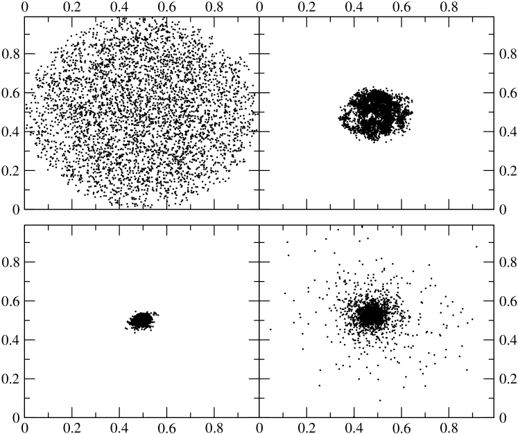
Figure 1: Snapshots of the evolution at from the cold sphere initial conditions described in the text. The first three snapshots are from the initial phase of contraction. Just after the third one (corresponding to $t=1$) the system reaches a minimal size, after which it “turns around”, ejecting some mass to infinity and binding the rest in a virialized structure shown in the last snapshot.

Qualitatively the evolution we observe in all our simulations is the same, and like that well known in both astrophysics, and, more generally, in statistical physics for systems with long-range attractive interactions from sub-virial initial conditions of this type (i.e. with an initial virial ratio larger than -1) : the system first contracts and relaxes “violently” (i.e. on timescales of order the dynamical time scale $\tau_{scm}$) to give a virialized, macroscopically stationary, state (see [3] for astrophysical references, and e.g. [4] for statistical physics references). Such states are known variously as “quasi-equilbria”, or “meta-equilibria” or “quasi-stationary” states, because they are understood not to be true equilibria, but rather stable only on a time scale which diverges as some power of $N$ — in proportion to $N/\log N$ for the case of gravity, according to simple arguments [12]. Indeed on these much longer timescales — which we do not explore here — the system is believed to be intrinsically unstable to so-called “gravothermal catastrophe” [13] (see, e.g., [14] for a recent exploration of this regime, and further references). We will use here the term “quasi-stationary states”, shortened to QSS, in line with the predominant usage in the statistical physics literature in the last few years.

Shown in Fig. 1 are four snapshots (with particle positions projected onto a plane) of a simulation with $N=4096$ particles at times $t=0$, $t=0.9$, $t=1$ and $t=2.5$. While at $t=1$ the system is still in the phase of contraction, at the last time it has already settled into the QSS. In Fig. 2 we show, for the simulations indicated (the notation $PN$ means $N$ Poisson distributed particles), the evolution of the virial ratio

$$b(t)=\frac{2K^{n}}{W^{n}}$$ (8)

where $K^{n}$ is the kinetic energy of the particles with negative energy, and $W^{n}$ the potential energy associated with the same particles. As we will discuss below, particles with positive energy are ejected completely from the system and thus they are not considered in Eq.8. We observe that the relaxation is remarkably rapid in time, with the bound particles “settling down” towards the QSS in considerably less than a further dynamical time $\tau_{scm}$ after the maximal “crunch”.

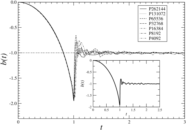
Figure 2: The virial ratio [see Eq.(8)] as a function of time for different simulations. In the insert panel is shown a “zoom” on the behavior of one of these curves around the time of collapse.

A typical evolution of the radial density profile is shown in Fig. 3: until close to the maximal collapsed configuration, it maintains, approximately, the top-hat form of the original configuration and then in a very short time changes and stabilizes to its asymptotic form . We will discuss the latter form and its dependence on $N$ below.

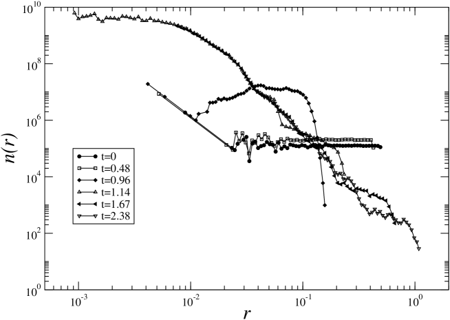
Figure 3: Density profile of particles with negative total energy at different times during the collapse, for a simulation with $N=65536$.

The existing studies in the astrophysical literature of this class of initial conditions [5, 6] focus on how the singular collapse of the uniform spherical collapse model is regulated at finite $N$, and in particular on the scaling with $N$ in numerical simulations of the minimal size reached by the system. Indeed in the study of [5] the “points” represent masses with extension (e.g. proto-stars) and the central question the authors wish to address is whether these masses survive or not the collapse of a cloud of which they are the constituents. (We note also the more recent study [7, 8] which focuses on the velocity distributions of the QSS.) This minimal radius $R_{min}$ may be defined in different ways, e.g., as the minimal value reached by the radius, measured from the center of mass, enclosing $90\%$ of the mass. Alternatively it can be estimated as the radius inferred from the potential energy of the particles, the minimal radius corresponding to the maximal negative potential energy. The behavior of $R_{min}$, determined by the first method, as a function of $N$ is shown in Fig. 4. The fitted line $R_{min}\propto N^{-1/3}$ is a behavior which has also been verified in both [5] and [6], the latter for an $N$ as large as $10^{7}$. As explained in these articles it is a behavior which can be predicted from very simple considerations. First, neglecting boundary effects (i.e. treating the limit of an infinite sphere), it can be shown that small density perturbations, in the fluid approximation, grow in proportion to $a^{-3/2}$ for $a<<1$. Second, the initial amplitude of the relative density perturbations scale in proportion to $N^{-1/2}$. If we assume that the uniform spherical collapse model breaks down when these perturbations to uniformity become of order unity — we arrive at the prediction $R_{min}\propto N^{-1/3}$. The same estimate can be given more physically as requiring a balance between the pressure forces, associated with the growing velocity dispersion, and the gravitational forces. Note that, in fact, $R_{min}\approx\ell$ as in our units $\ell=0.5/N^{1/3}$, i.e. the minimal size reached by the system is not just proportional to, but in fact approximately equal to, the initial inter-particle separation.

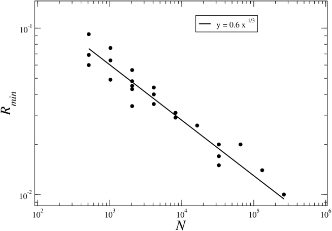
Figure 4: Behavior of the minimal radius $R_{min}$ attained, determined as described in text, as a function of $N$. The solid line corresponds to the prediction described in the text.

Let us consider now the scaling with $N$ of various other fundamental quantities, a question which has not been considered in previous works. Specifically we focus on the macroscopic characterization of the QSS formed in all cases. Let us consider first the mass and energy: while all particles start with a negative energy, a finite fraction can in fact end up with a positive energy. Given that they move, from very shortly after the collapse, in the essentially time independent potential of the virialized (negative energy) particles, they escape from the system. While evidently the ejected mass is bounded above by the initial mass, the ejected energy is, in principle, unbounded above as the gravitational self energy of the bounded final mass is unbounded below.

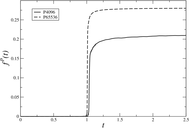
Figure 5: The behavior of $f^{p}(t)$, the fraction of the particles with positive energy, as a function of time for two different simulations. A dependence on the number of particles is manifest.

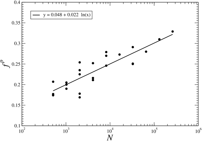
Figure 6: Behavior of the fraction of ejected particles as a function of the total number of particles in the system. The solid line is the phenomenological fit given by Eq. (9).

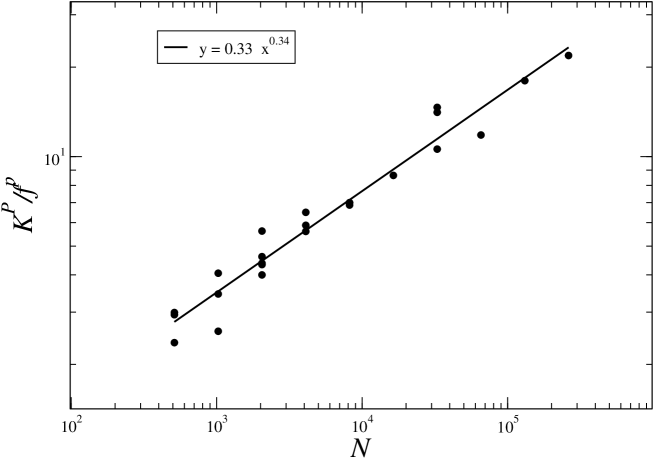
Figure 7: Observed behavior of the ratio $K^{p}/f^{p}$ as a function of $N$.

That ejection of mass and energy indeed takes place, that it is non-negligible, and $N$ dependent, is shown in Figs. 5,  6 and  7. The first figure shows the fraction $f^{p}$ of the particles with positive energy as a function of time in two different simulations, while the second shows the asymptotic value of $f^{p}$ in each simulation as a function of $N$ (i.e. the value attained on the “plateau” in each simulation after a few dynamical times, corresponding to particles which are definitively ejected on these time scales.)

Although $f^{p}$ fluctuates in different realizations with a given particle number, it shows a very slow, but systematic, increase as a function of $N$, varying from approximately $15\%$ to almost $35\%$ over the range of $N$ simulated. A reasonably good fit is given by

$$f^{p}(N)\approx a+b\log(N)\;,$$ (9)

where $a=0.048$ and $b=0.022$. Alternatively it can be fit quite well (in the same range) by a power law $f^{p}\approx 0.1N^{0.1}$. Note that these fits cannot, evidently, be extrapolated to arbitrarily large $N$ (as the mass ejected is bounded above), and thus our study does not actually definitively determine the asymptotic large $N$ behavior of this quantity despite the large particle numbers simulated. As we will discuss briefly below, however, the mechanism we observe for this mass ejection leads us to expect that the value of $f^{p}$ should saturate when $f^{p}\sim 0.5$.

Fig.  7 shows the ratio $K^{p}/f^{p}$, i.e., the kinetic energy per unit ejected mass, as a function of $N$. It has a much clearer and well defined growth as a function of $N$, well fit by $K^{p}/f^{p}\propto N^{1/3}$. Note that for the largest values of $N$ simulated $K^{p}$ is almost ten times the initial (potential) energy $E_{0}$ of the system.

The increasing ejection of energy means that the particles which remain in the QSS become more and more bound as $N$ increases. Indeed using total energy conservation, and the fact that both the final potential energy of the ejected particles and that associated with the interaction of the bound and ejected particles is negligible, we have

$$E_{0}=W^{n}+K^{p}+K^{n}\;.$$ (10)

Further, since the bound particles in the QSS are virialized we have

$$2K^{n}+W^{n}=0\;.$$ (11)

Thus we have

$$W^{n}=-2K^{n}=2(E_{0}-K^{p})$$ (12)

so that we have the approximate behavior $W^{n}\propto-N^{-1/3}$ (when we neglect the slow observed variation with $N$ of $f^{p}$).

The dependence of the ejected energy on $N$ thus implies that the macroscopic properties of the QSS also depend on $N$. Studying the radial density profiles of the (approximately spherically symmetric) QSS we find that they can always be fit well by the simple functional form

$$n(r)=\frac{n_{0}}{\left(1+\left(\frac{r}{r_{0}}\right)^{4}\right)}\;.$$ (13)

The $N$ dependence is encoded in that of the two parameters $n_{0}$ and $r_{0}$, which we find are well fit by $r_{0}\propto N^{-1/3}$ and $n_{0}\propto N^{2}$. In Fig. 8 we show the density profiles for various simulations with different $N$ where the axes have been rescaled using these behaviors.

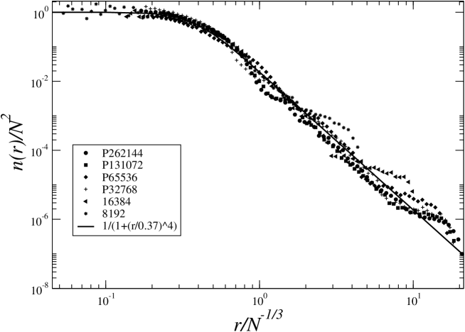
Figure 8: Density profile of the virialized structure at a time $t\approx 4\tau_{scm}$ for simulations with different number of particles. The y-axis has been normalized by $N^{2}$ and the x-axis by $N^{-1/3}$ (see text for explanations). The behavior of Eq. (13) is shown for comparison.

It is simple to show that these scalings with $N$ of $n_{0}$ and $r_{0}$ are simply those which follow from those just given for $f^{p}$ and $W^{n}$: using the ansatz Eq. (13) one has that the number $N^{n}$ of bound particles is proportional to $n_{0}r_{0}^{3}$ while the potential energy $W^{n}$ is proportional to $m^{2}n_{0}^{2}r_{0}^{5}$ where $m$ is the mass of a particle. The best fit behaviors for $r_{0}$ and $n_{0}$ thus correspond, since $m\propto 1/N$, to $N^{n}\sim N$ (i.e. a constant bound mass, and therefore a constant ejected fraction of the mass $f^{p}$) and $W^{n}\sim N^{1/3}$. More detailed fits to $n_{0}$ and $r_{0}$ show consistency also with the very slow variation of $f^{p}$ observed. In summary the $N$ dependence of the QSS manifests itself to a very good approximation simply in a scaling of its characteristic size in proportion to $R_{min}$, the minimal radius attained in the collapse (which, as we have seen, is proportional to the initial inter-particle separation).

2.2 Dynamics of ejection

\psfrag{X}[c]{$t$}\psfrag{Y}[c]{Arbitrary units}\includegraphics*[width=325.215pt]{FIG9.eps}

Figure 9: Radial velocity, and average energy per particle, as a function of time, of particles which are bound/ejected at the end of the simulation of $131072$ particles. The energy of the particles has been arbitrarily rescaled.

We have investigated in detail the evolution of the system during collapse and have identified the mechanism which leads to the mass and energy ejection we have just described. We limit ourselves here to a very brief qualitative description of our results, of which the full details are reported in [3]. The probability of ejection is closely correlated with particles’ initial radial positions, with essentially particles initially in the outer shells being ejected. The reason why these particles are ejected can be understood as follows. Firstly, particles closer to the outer boundary systematically lag (in space and time) with respect to their uniform spherical collapse trajectories more than those closer to the center. This is an effect which arises from the fact that, when mass moves around due to fluctuations about uniformity, there is in a radial shell at the boundary no average inward flux of mass to compensate the average outward flux. The mean mass density thus seen by a particle in such a shell just decreases, leading to a slow of its fall towards the origin. This “lag” with respect to particles in the inner shells propagates in from the boundaries with time, leading to a coherent relative lag of a significant fraction of the mass by the time of maximal compression. Secondly, these lagging particles are then ejected as they pick up energy, in a very short time around the collapse, as they pass through the time-dependent potential of the particles initially closer to the center, which have already collapsed and “turned around”. This is illustrated in Fig. 9, which shows, for a simulation with $N=131072$ particles, the temporal evolution of the components of the mass which are asymptotically ejected or bound. More specifically the plot shows the evolution of $v_{e}$ (and $v_{b}$) which is the average of the radial component of the velocity for the ejected (and bound) particles, and also e_e (and e_b) which is the mean energy per ejected (and bound) particle (i.e. the average of the individual particle energies). The behaviors of $v_{e}$ and $v_{b}$ show clearly that the ejected particles are those which arrive on average late at the center of mass, with $v_{e}$ reaching its minimum after the bound particles have started moving outward. Considering the energies we see that it is in this short time, in which the former particles pass through the latter, that they pick up the additional energy which leads to their ejection. Indeed the increase of $e_{e}$ sets in just after the change in sign of $v_{b}$, i.e., when the bound component has (on average) just “turned around” and started moving outward again. The mechanism of the gain of energy leading to ejection is simply that the outer particles, arriving later on average, move through the time dependent decreasing mean field potential produced by the re-expanding inner mass. Assuming that the fraction of the lagging mass is independent of $N$, an analysis of the scaling (see [3]) of the relevant characteristic velocity/time/length scales allows one to infer the observed scaling of the ejected energy with $N$. Quantitatively we have not been able to explain, on the other hand, the observed $N$ dependence of the lagging mass, which should determine the $N$ dependence of $f^{p}$. Given, however, that it is determined by a lag of the outer mass relative to that of the inner mass, it seems clear that, as required, the mechanism observed will naturally lead it to saturate at a fixed fraction, of order one, as $N$ increases arbitrarily.

2.3 Discussion

In theoretical attempts to understand the properties of QSS produced by violent relaxation using a statistical mechanics approach — whether the original one of Lynden-Bell [17] or variants thereof — two assumptions are generally made: 1) the mass and energy of the virialized state is equal to the initial values of these quantities, and 2) the dynamics is “collisionless”, i.e., described by the Vlasov-Poisson equations for the one particle phase space density.

The first assumption is clearly not valid for the class of initial conditions we have studied, not even as a first approximation. Although the ejection we have observed, and in particular its behavior with $N$, is clearly a result of the extreme violence of the collapse due to the cold initial conditions, we do not expect such ejection to be a feature only of this particular initial condition. In a preliminary study of initial conditions incorporating an initial velocity dispersion, we have found significant ejection until an initial virial ratio of close to $0.5$ is reached. Thus, in general, any such statistical approach to explaining the properties of the virialized states should take into account in principle that the dynamical evolution can change the values of the effective mass and energy which is available for relaxation. This observation is, we believe, in line with the findings by Y. Levin et al. reported at this conference (see also [18]): using studies of both Coulomb and self-gravitating systems, they argue that the Lynden-Bell approach works well when the violent relaxation is “gentle”, but that when it is violent the effects of resonances in the dynamics lead to separation of part of the mass into a “halo” which does not relax to the prescribed statistical equilibrium. We note that a similar conclusion has been reached in earlier work on the $1-d$ “sheet model” (see e.g. [19]). In the case we have studied there is a “dynamical resonance” between the inner collapsing core and the outer lagging particles in the collapse, leading to the complete ejection of these particles from the system. In this context we note that none of these findings should change if we consider, as required notably in the Lynden-Bell framework, a system enclosed in a finite volume instead of an open one: if we put our system in a box, the ejected component will simply bounce off the walls and remain as an unbound cloud moving in and out of the time independent potential of the “core”.

A second assumption of importance in theoretical models is that the evolution of the system is well described by the coupled Vlasov-Poisson (VP) equations (or “collisionless Boltzmann equation” coupled to the Poisson equation). Is this the case? To determine whether it is we need to understand how we can test for its validity. As the VP limit is an appropriate $N\rightarrow\infty$ limit for the system, this means specifying precisely how this limit should be taken. We can then extrapolate our numerical simulations to larger $N$ to test for the stability of results.

It is clear that the appropriate extrapolation for the system we have studied is not the naive limit $N\rightarrow\infty$, i.e., in which we simply increase the number of Poisson distributed particles: we have explicitly identified macroscopic $N$ dependencies in fundamental quantities, so the results at any given $N$ do not approximate those at any other $N$, and indeed do not converge towards any $N$-independent behavior.

Formal proofs of the validity of the VP limit [20] for a self-gravitating system require, however, that the singularity in the gravitational force at zero separation be regulated when the limit $N\rightarrow\infty$ is taken. This suggests we should take the limit $N\rightarrow\infty$ while keeping fixed a smoothing scale, like the $\varepsilon$ we have introduced in our simulations. Doing so we would indeed expect to obtain a well defined $N$-independent result, corresponding to the uniform spherical model with such a regularization of the force: the sphere will not collapse below a radius of order $\varepsilon$, as the force is then weaker than the Newtonian force (and goes asymptotically to zero). One would then expect to obtain, for sufficiently large $N$, a final state which is well defined and $N$ independent, but dependent on the scale of the regularization and indeed even on the details of its implementation.

This limit is not the VP limit relevant here. We have indeed introduced a regularization of the force, but this has been done, as we have discussed, only for reasons of numerical convenience, and our criterion for our choice of $\varepsilon$ is that it be sufficiently small so that our numerical results are independent of it. Our results are thus, a priori, independent of the scale $\varepsilon$ (and of how the associated regularization is implemented). To illustrate this we show in Fig. 10 the evolution of $f^{p}$ (the fraction of particles with positive energy) as a function of time, in simulations from identical initial conditions with $N=32768$ particles in which only the value of $\varepsilon$ has been varied, through the values indicated.

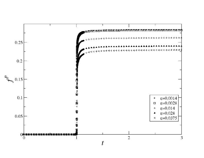
Figure 10: Evolution of the fraction of the mass with positive energy for simulations with $N=32768$ for the different values indicated of the smoothing parameter $\varepsilon$.

Other quantities we have considered show equally good convergence as $\varepsilon$ decreases. Note that for the given simulation the mean inter-particle distance in our units is $\ell=0.016$, so that the convergence of results is attained once $\varepsilon$ is significantly less than $\ell$. As we have seen, the minimal size reached by the collapsing system scales in proportion to $\ell$. We interpret the observed convergence as due to the fact that the evolution of the system is determined primarily by fluctuations on length scales between this scale and the size of the system. Once $\varepsilon$ is sufficiently small to resolve these length scales at all times, convergence is obtained.

Given the essential role played by fluctuations to the mean density in determining the final state, it is clear that only an extrapolation of $N$ which keeps the fluctuations in the initial conditions fixed can be expected to leave the macroscopic results invariant. Any change in $N$ necessarily leads, however, to some change in the fluctuations. If, however, as indicated by the above results, there is a minimal length scale in the initial conditions for “relevant” fluctuations, we expect an extrapolation of $N$ which leaves fluctuations above this minimal scale unchanged to give stable results.

Such an extrapolation for our initial conditions can be defined as follows. Starting from a given Poissonian initial condition of $N$ particles in a sphere, we create a configuration with $N^{\prime}=nN$ particles by splitting each particle into $n$ particles in a cube of side $2r_{s}$, centered on the original particle. The latter particles are distributed randomly in the cube, with the additional constraint that their center of mass is located at the center of the cube, i.e., the position of the center of mass is conserved by the “splitting”. In this new point distribution, which has the same mean mass density as the original distribution, fluctuations on scales larger than $r_{s}$ are essentially unchanged compared to those in the original distribution, while fluctuations around and below this scale are modified (see [21] for a detailed study of how fluctuations are modified by such “cloud processes”.). We have performed this experiment for a Poisson initial condition with $N=4096$ particles, splitting each particle into eight ($n=8$) to obtain an initial condition with $N^{\prime}=32768$ particles. Results are shown in Fig. 11 for the ejected mass as a function of time, for a range of values of the parameter $r_{s}$, expressed in terms of $\ell$, the mean inter-particle separation (in the original distribution). While for $r_{s}=0.8\ell$ the curve of ejected particles is actually indistinguishable in the figure from the one for the original distribution, differences can be seen for the other values, greater discrepancy becoming evident as $r_{s}$ increases. This behavior is clearly consistent with the conjecture that the macroscopic evolution of the system depends only on initial fluctuations above some scale, and that this scale is of order the initial inter-particle separation $\ell$. And, as anticipated, this translates into an $N$ independence of the results when $N$ is extrapolated in this way for an $r_{s}$ smaller than this scale.

This prescription for the VP limit can be justified theoretically using a derivation of this limit through a coarse-graining of the exact one particle distribution function over a window in phase space (see e.g. [22]). The VP equations are obtained for the coarse-grained phase space density when terms describing perturbations in velocity and force below the scale of the coarse-graining are neglected. A system is thus well described by this continuum VP limit if the effects of fluctuations below some sufficiently small scale play no role in the evolution. The definition of the limit thus requires explicitly the existence of such a length scale, and the limit is approached in practice when the mean inter-particle distance becomes much smaller than this scale. With the kind of procedure given we have defined not only an extrapolation of $N$ which gives stable results, but also a method of identifying this scale.

\psfrag{X}[c]{ \large$t$}\psfrag{Y}[c]{ \large$f^{p}$}\includegraphics*[width=341.43306pt]{FIG11.eps}

Figure 11: Evolution of the fraction of particles with positive energy as a function of time, for the different indicated values of the parameter $r_{s}$ described in text. The “original” initial conditions has $4096$ particles while the others have $32768$ particles. The curve for $r_{s}=0.8$ is not visible because it is superimposed on that of the original distribution.

3 The infinite system limit

Let us consider now the infinite system limit, i.e. the usual thermodynamic limit in which $N\rightarrow\infty$ and $V\rightarrow\infty$ at fixed particle density. This is the limit relevant in the context of structure formation in the universe. In a Newtonian framework this limit is not uniquely defined for the simple reason that the sum giving the force on a particle on the right hand side of Eq. (1) is not defined when the distribution of points summed over is infinite with a non-zero mean density. By giving appropriate prescriptions for the calculation of this sum — or equivalently, by giving a prescription for how the size of the system is extrapolated — one can define, however, the dynamical problem in an infinite distribution. There are two simple possibilities for such a prescription. One gives exactly the equations for particle motion used in cosmological $N$- body simulations of the expanding universe, the other defines the same problem in a static universe. Although the latter of is less direct practical relevance, it is, as we will discuss, an interesting case for theoretical study, providing a simplified framework in which to approach the full cosmological problem.

The case of an expanding (or contracting) universe is simply a limit of the finite problem we have just studied. The uniform cold spherical collapse model, which is the simple $N\rightarrow\infty$ limit of the finite initial condition we have studied, is, as we have discussed, singular at $t=\tau_{scm}$. At all times $t<\tau_{scm}$ it is, however, well defined for any size of the (spherical) system, and independently of this size. Until a time of order the maximal collapse in any finite $N$ system the trajectories of the particles are, to a first approximation, those in the uniform limit and it is thus useful to study the problem in “comoving coordinates” defined, for the $i$-th particle with position vector ${\bf r}_{i}(t)$ by ${\bf x}_{i}(t)={\bf r}_{i}(t)/a(t)$. The equations of motion Eqs. (1) then become, using Eq. (3),

$$\ddot{\bf x}_{i}+\frac{\dot{a}}{a}\dot{\bf x}_{i}=-\frac{1}{a^{3}}\left[\sum_{j\neq i}\frac{Gm({\bf x}_{i}-{\bf x}_{j})}{|{\bf x}_{i}-{\bf x}_{j}|^{3}}-\frac{4\pi G}{3}\rho_{0}{\bf x}_{i}\right]\,.$$ (14)

Now, in contrast to the force in Eq. (1), the expression inside the brackets on the right-hand side, can be shown to be well defined in a broad class of infinite point distributions: the subtracted term removes the divergent term in the force arising from the average density $\rho_{0}$. Specifically, for example, this regularized force is known to be well defined in an infinite Poisson distribution, in which case it is characterized by the so-called Holtzmark distribution first derived by Chandrasekhar [23].

We can thus define an infinite volume limit for the system, as that in which the equations of motion are given by Eqs. (14) with the sum in the “force” taken over an appropriate infinite system (i.e. in the class in which it is defined). In order that $a(t)$ have the physical significance it has in the case of a finite sphere, the prescription on the force is that it be calculated by summing in spheres about the chosen origin. The generalization to an expanding universe is obtained simply by taking an appropriate expanding initial condition on the motion of the particles, i.e., with initially outward velocities proportional to the particles’ positions with respect to the origin. As we noted above this gives the appropriate Friedmann equation (6) for $a(t)$. The case $\kappa=0$ corresponds to the so called Einstein-de Sitter universe, with $a(t)\propto t^{2/3}$.

With respect to the problem we have studied above, the infinite space limit defined in this way thus describes the development of the clustering inside the contracting (or expanding) sphere in the temporal regime in which the finite-size effects we have described briefly above — which lead to the regularization of the singularity in the finite case — are negligible. Indeed in our simulations we find that the finite size effects we identified, of systematic particle lag with respect to the uniform spherical collapse model, propagate at a given time a radial distance into the interior of sphere which decreases as $N$ increases. Thus as we take the boundary of the sphere to infinity we approach a well defined and non-trivial limit for the particle trajectories at any time $t<\tau_{scm}$, in which the regime we have studied for the finite system simply disappears.

When the regulated force term on the right-hand side of Eqs. (14) is well defined in an infinite distribution, they can be conveniently rewritten as

$$\ddot{\bf x}_{i}+\frac{\dot{a}}{a}\dot{\bf x}_{i}=-\frac{Gm}{a^{3}}\lim_{R_{s}\rightarrow\infty}\sum_{j\neq i,j\in V(R_{s},{\bf x}_{i})}\frac{{\bf x}_{i}-{\bf x}_{j}}{|{\bf x}_{i}-{\bf x}_{j}|^{3}}\,,$$ (15)

where $V(R_{s},{\bf x})$ is a sphere of radius $R_{s}$ centered on the point with comoving position ${\bf x}$. When the sum is performed in this way — symmetrically about each particle — the contribution from the mean density vanishes. These are the equations used in simulations of structure formation in the universe, with the particles initially perturbed slightly from an infinite perfect lattice, with small velocities in comoving coordinates. (The infinite system is treated, in practice, as we will discuss below, using the “replica method” in which the force is calculated in an infinite periodic system).

While, following the derivation given of these equations, the function $a(t)$ should be a solution of Eq. (6), when the system is treated directly in comoving coordinates this function is in practice inserted “by hand” (for the appropriate cosmology) and the results for the clustering from given initial conditions depend on it. Formally, however, one can insert any function $a(t)$ and study the evolution of the clustering. A particularly interesting case, which we will describe below, is when $a(t)=1$, i.e., a static universe. It is not a solution to Eq. (6) simply because no exactly uniform distribution of purely self-gravitating matter in a finite sphere (or indeed any geometry) is static.

This choice corresponds to what is known as the “Jeans’ swindle” [24, 12]: To treat the dynamics of perturbations to an infinite self-gravitating pressure-full fluid, Jeans “swindled” by perturbing about the state of constant mass density and zero velocity, which is not, in fact a solution of these fluid equations. Formally the “swindle” involves removing the mean density from the Poisson equation, so that the gravitational potential is sourced only by fluctuations to this mean density. From Eq. (15) with $a(t)=1$ it is manifest that this is equivalent to the prescription that the gravitational force in an infinite distribution be calculated by summing symmetrically about each point. As discussed by Kiessling [25], the presentation of what Jeans did as a “mathematical swindle” is in fact misleading: formulated in this way as a regularization of the force — that which makes the force zero in an infinite uniform distribution — it is perfectly well defined mathematically. The mathematical inconsistency in Jeans’ analysis arises because it is done in terms of potentials which are always badly defined in the infinite volume limit, whereas forces, which are the physically relevant quantities, may remain well defined. Kiessling notes that an equivalent form of the Jeans’ “swindle” prescription for the force on a particle is

$${\bf F}({\bf r}_{i})=-{Gm}\lim_{\mu\rightarrow 0}\sum_{j\neq i}\frac{{\bf r}_{i}-{\bf r}_{j}}{|{\bf r}_{i}-{\bf r}_{j}|^{3}}e^{-\mu|{\bf r}_{i}-{\bf r}_{j}|}$$ (16)

where the sum now extends over the infinite space. This prescription is an alternative to the one given above, which employs a sharp spherical top-hat window. Both prescriptions (which give the same result, identical to the Jeans’ “swindle”) are simply regularizations of the Newtonian force in the infinite volume (thermodynamic) limit different to the spherical summation prescription which we have seen lead to the expanding/contracting universe. The formulation in terms of a limiting procedure on a screened potential is, however, very useful in that it gives a clearer physical meaning to this infinite system limit: it means that the dynamics we observe in this limit — which we will describe for a simple class of initial conditions below — is the dynamics one would observe in a screened gravitational potential starting from such an initial condition, up to a time when the length scales which characterize this dynamics becomes of order the screening length. In practice, as we will now see, the relevant scale is the “scale of non-linearity”.

4 Dynamics of an infinite system

We now describe the dynamical evolution of an infinite, initially quasi-uniform, distribution of self-gravitating particles in a static universe, i.e., with equations of motion which can be written as

$$\ddot{{\bf r}}_{i}=-{Gm}\lim_{\mu\rightarrow 0}\sum_{j\neq i}\frac{{\bf r}_{i}-{\bf r}_{j}}{|{\bf r}_{i}-{\bf r}_{j}|^{3}}e^{-\mu|{\bf r}_{i}-{\bf r}_{j}|}\,.$$ (17)

In practice one can simulate numerically, of course, the motion of only a finite number of particles. Following the discussion in the previous section, we could in principle recover the relevant dynamics up to any time from simulations of an appropriate sufficiently large finite system with open boundary conditions. Indeed we could use the simulations discussed above for cold spherical collapse from Poissonian initial conditions to study the dynamics of an infinite contracting universe from Poissonian initial conditions: this dynamics will be well approximated, as we have discussed, for a time prior to the global collapse which increases as $N$ does. The case of a static universe which we wish to consider, on the other hand, would require that the gravitational interaction be screened on a scale considerably smaller than the system size. This would prevent the global collapse, but the dynamics will only approximate that in the infinite volume limit as long as the clustering which develops is at a scale sufficiently smaller than the screening scale. Instead of such a procedure it is much simpler to study numerically a system which is infinite, but periodic, i.e., a finite cubic box and an infinite number of copies. This method, standard in cosmological simulations, as well as in simulations of Coulomb systems in statistical physics, is known as the “replica method”. As the sum for the force in Eq. (17) is convergent it can be evaluated numerically with desired precision in this infinite distribution. This is usually done using the so-called Ewald sum method (see e.g. [26]). The results given here have been obtained, as above, using the publicly available GADGET2 code [9, 10, 11], which allows also the treatment of infinite periodic systems based on this method.

As initial conditions for our study, which is reported in much greater details in [27, 28, 29], we consider, for reasons we will now explain, the following class of “shuffled lattice” (SL) distributions, defined as follows: particles initially on a perfect lattice, of lattice spacing $\ell$ (= mean inter-particle spacing), are displaced randomly (“shuffled”) about their lattice site independently of all the others. A particle initially at the lattice site $\mathbf{R}$ is then at $\mathbf{x}(\mathbf{R})=\mathbf{R}+\mathbf{u}(\mathbf{R})$, where the random vectors $\mathbf{u}(\mathbf{R})$ are specified by $p(\mathbf{u})$, the PDF for the displacement of a single particle. We use a simple top-hat form for the latter, i.e., $p({\bf u})=(2\Delta)^{-3}$ for ${\bf u}\in[-\Delta,\Delta]^{3}$, and $p({\bf u})=0$ otherwise . Taking $\Delta\to 0\,$, at fixed $\ell$, one thus obtains a perfect lattice, while taking $\Delta\to\infty$ at fixed $\ell$, gives a Poisson particle distribution [30].

Given that we will be studying behaviors of the periodic system which are independent of the size of the cubic box (i.e. representative of the truly infinite SL as just defined), and that the (unsmoothed) gravitational interaction itself defines no characteristic scale, our chosen class of initial conditions is actually characterized by a single parameter, which we may choose to be the dimensionless ratio $\delta\equiv\Delta/\ell$, which we will refer to as the normalized shuffling parameter. Note that, in contrast to the finite case, a Poissonian initial condition thus defines only a single initial condition as in the infinite system limit it is characterized solely by the mean inter-particle spacing which can always be taken as unit of length (in the absence of a system size which defines an independent length scale, and assuming that any small-scale smoothing of the interaction introduced plays no significant role in the dynamics on the time scales considered).

To characterize the correlation properties of the SL, and those of the evolved configurations, a useful quantity is the power spectrum (or structure factor). We recall that for a point (or continuous mass) distribution in a cube of side $L$, with periodic boundary conditions, it is defined as (see e.g. [30])

$$P(\mathbf{k})=\frac{1}{L^{3}}\langle|\tilde{\delta}(\mathbf{k})|^{2}\rangle\,,$$ (18)

where $\tilde{\delta}(\mathbf{k})$ are the Fourier components of the mass density contrast, which, for particles of equal mass, is simply

$$\tilde{\delta}(\mathbf{k})=\frac{1}{n_{0}}\sum_{i=1}^{N}\exp(-i\mathbf{k}\cdot{\mathbf{x}}_{i})\,,$$ (19)

for $\mathbf{k}=(2\pi/L)\mathbf{n}$, where $\mathbf{n}$ is a vector of integers, $n_{0}$ is the mean number density and the sum is over the $N$ particles (with the $i$-th at ${\mathbf{x}}_{i}$). Note that with this normalization, which is that used canonically in cosmology, the asymptotic behavior at large $\mathbf{k}$ in any point process is $P(\mathbf{k}\rightarrow\infty)=\frac{1}{n_{0}}$. It is straightforward to calculate analytically the power spectrum for a generic SL. Expanded in Taylor series about $\mathbf{k}=0$ gives the leading small-$k$ behavior

$$P(\mathbf{k})\approx\frac{k^{2}\Delta^{2}}{3n_{0}}=\frac{1}{3}k^{2}\delta^{2}\ell^{5}\,,$$ (20)

where $k=|\mathbf{k}|$. Note that this small-$k$ behavior of the power spectrum of the SL therefore does not depend on the details of the chosen PDF for the displacements, but only on its (finite) variance.

This class of SL initial conditions has the interest also that, while simplified, they resemble those standardly used in cosmological simulations. In this context initial conditions are prepared by applying correlated displacements to a lattice. By doing so one can produce, to a good approximation, a desired power spectrum at small wave-numbers (See [31] for a detailed description and analysis). The amplitude of the relative displacements at adjacent lattice sites is then related to the amplitude of the initial (very small) density fluctuations at the associated physical scale. In the SL this translates into the fact that, from Eq. (20), the amplitude of the power spectrum at small $k$ is a simple (quadratic) function of the normalized shuffling $\delta$.

A full analysis of simulations for a range of different $\delta$ can be found in [27]. As we wish here principally to illustrate the qualitative features of the evolution for a value of $\delta$ typical of a cosmological simulation we will present results just for a single case, $\delta=1$. We will then discuss the effect of the variation of $\delta$ in the context of our discussion of the validity of the VP limit.

The results we give now are for two $\delta=1$ simulations: SL64, with $64^{3}$ particles, and SL128, with $128^{3}$ particles of the same mass. We choose as unit of length that in which the box size in one in SL64, and two in SL128, i.e., the lattice spacing (and average mass density) is fixed and the simulations thus differ only in the box size. These simulations can be used to check that the dynamics is indeed independent of the box size, and the results below are for the temporal regime in which this is the case (i.e. in which the quantities considered are in good agreement in the two simulations). As in our finite system simulations we use, for numerical efficiency, a non-zero smoothing $\varepsilon$, of which the value in the SL64 and SL128 runs reported is $\varepsilon=0.00175$ which corresponds to $\varepsilon\approx 0.1\ell$. As in this case we have tested that our results are stable to the use of smaller values of $\varepsilon$. The particles are again assigned zero velocity at the initial time, $t=0$.

4.1 Results

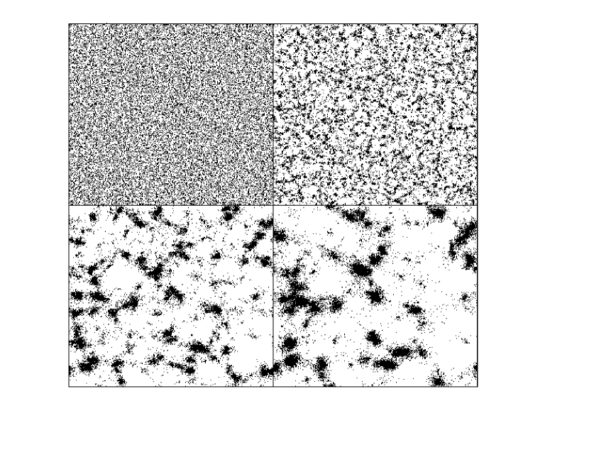
Figure 12: Snapshots of SL64, at $t=0$, and the evolved configurations obtained at subsequent times, t=$3,6,8$. (These are projections onto the $x-y$ plane of a thin orthogonal slice of the full cube).

In Fig. 12 are shown four snapshots of the simulation SL64. The time units here are slightly different than those used in the finite spherical collapse simulations, the unit of time being approximately $\tau_{scm}/2$ (see [27] for the exact definition employed). We see visually that non-linear structures (i.e. regions of strong clustering) appear to develop first at small scales, and then propagate progressively to larger scales. Eventually the size of the structures become comparable to the box-size. From this time on the evolution of the system will no longer be representative of that in the infinite system. Up to close to this time, however, it is indeed the case that all the properties we will study below show negligible dependence on the box size (see Refs. [27, 28] for more detail).

Let us consider first the evolution of clustering in real space, as characterized by the reduced correlation function $\xi(r)$. We recall that this is simply defined as

$$\xi(\mathbf{r})=\langle\delta(\mathbf{x}+\mathbf{r})\delta(\mathbf{x})\rangle\;,$$ (21)

where $\langle...\rangle$ is an ensemble average, i.e., an average over all possible realizations of the system (and we have assumed statistical homogeneity). It is useful to note that this can be written, for $r\neq 0$, and averaging over spherical shells,

$$\xi(r)=\frac{\langle n(r)\rangle_{p}}{n_{0}}-1\;,$$ (22)

where $\langle n(r)\rangle_{p}$ is the conditional average density, i.e., the (ensemble) average density of points in an infinitesimal shell at distance $r$ from a point of the distribution. Thus $\xi(r)$ measures clustering by telling us how the density at a distance from a point is affected, in an average sense, by the fact that this point is occupied. In distributions which are statistically homogeneous the power spectrum $P(\mathbf{k})$ and $\xi(\mathbf{r})$ are a Fourier conjugate pair (see e.g. Ref. [30]).

The correlation functions here will invariably be monotonically decreasing functions of $r$. It is then useful to define the scale $\lambda$ by

$$\xi(\lambda)=1\,.$$ (23)

This scale then separates the regime of weak correlations (i.e. $\xi(r)\ll 1$) from the regime of strong correlations (i.e. $\xi(r)\gg 1$). In the context of gravity these correspond, approximately, to what are referred to as the linear and non-linear regimes, as a linearized treatment of the evolution of density fluctuations (see below) is valid in the former case. Eq. (23) can also clearly be considered as a definition of the homogeneity scale of the system. Physically it gives then the typical size of strongly clustered regions.

In Fig. 13 is shown the evolution of the absolute value $|\xi(r)|$ in a log-log plot, for the SL128 simulation.

Figure 13: Behavior of the absolute value of the correlation function $|\xi(r)|$ in SL128 at times $t=0,1,2,4,6,8$. The vertical dotted line indicates $\varepsilon$. From [27].

These results translate quantitatively the visual impression gained above. More specifically we observe that:

• Starting from $\xi(r)\ll 1$ everywhere, non-linear correlations (i.e. $\xi(r)\gg 1$ ) develop first at scales smaller than the initial inter-particle distance.

• After two dynamical times the clustering develops little at scales below $\varepsilon$. The clustering around and below this scale is characterized by an approximate “plateau”. This corresponds to the resolution limit imposed by the chosen smoothing.

• At scales larger than $\varepsilon$ the correlations grow continuously in time at all scales, with the scale of non-linearity [which can be defined, as discussed above, by $\xi(\lambda)=1$] moving to larger scales.

Once significant non-linear correlations are formed, the evolution of the correlation function $\xi(r,t)$ can in fact be described, approximately, by a simple spatio-temporal scaling relation:

$$\xi(r,t)\approx\Xi\left(r/R_{s}(t)\right)\,,$$ (24)

where $R_{s}(t)$ is a time dependent length scale which we discuss in what follows.

Figure 14: Collapse plot of $\xi(r,t)$: for each time $t>1$ we have rescaled the $x$-axis by a time-dependent factor to collapse all the curves (dashed ones) to that at time $t=1$. We have added for comparison $\xi(r,t=8)$ without rescaling (“w. resc.”, continuous line). From [27].

Shown in Fig. 14 is “collapse plot” which allows one to evaluate the validity of this relation: $\xi(r,t)$ at different times is represented with a rescaling of the $x$-axis by a (time-dependent) factor chosen to superimpose it as closely as possible over itself at $t=1$, which is the time from which the “translation” appears to first become a good approximation. We can conclude clearly from Fig. 14 that the relation Eq. (24) indeed describes very well the evolution, down to separations of order $\varepsilon$, and up to scales at which the noise dominates the estimator (see [27] for further details).

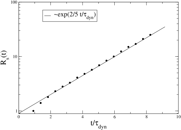
Figure 15: Evolution of the function $R_{s}(t)$ in SL128 (points) compared with its prediction from linearized fluid treatment, as explained in the next section. From [27].

In Fig. 15 is shown the evolution of the rescaling factor $R_{s}(t)$ found in constructing Fig. 14, as a function of time [with the choice $R_{s}(1)=1$]. The theoretical curve also shown, which fits the data very well at all but the earliest times, is that inferred from a simple analysis analogous to that used in cosmology for the expanding universe (see e.g. [32]), which we now describe. In this context, this spatio-temporal scaling behavior of the correlations is known as self-similarity. It has been observed in cosmological N body simulations starting from a range of initial conditions characterized by a simple power-law PS (see e.g. [33, 34]).

Firstly we need the result of the standard “linear theory” in cosmology. When the equations for the density and velocity perturbations in an infinite self-gravitating pressure-less fluid (which can be obtained by an appropriate truncation of the VP equations) are solved perturbatively, one obtains, in the static universe case, simply

$$\ddot{\delta}(\mathbf{x},t)=4\pi G\rho_{0}\delta(\mathbf{x},t)\,\,{\rm and}\,\,\ddot{\tilde{\delta}}(\mathbf{k},t)=4\pi G\rho_{0}\tilde{\delta}(\mathbf{k},t)\$$ (25)

which, for the case of zero initial velocities, gives

$$\delta(\mathbf{k},t)=\delta(\mathbf{k},0)\cosh\left(\sqrt{4\pi G\rho_{0}}\ t\right)\;.$$ (26)

and thus for the power spectrum

$$P(\mathbf{k},t)=P(\mathbf{k},0)\cosh^{2}\left(t/\tau_{\rm{dyn}}\right)\,.$$ (27)

where we have defined $\tau_{\rm{dyn}}=1/\sqrt{4\pi G\rho_{0}}$. That this indeed describes well the evolution of the power spectrum at sufficiently small wave-numbers can be seen from Fig. 16, which shows this quantity for the SL128 simulation along with the prediction of Eq. (27).

Figure 16: Evolution of the power spectrum in SL128 (solid lines — label FG): the curves are for time equal to 0,2,4,6,8 (from bottom to up). The dashed lines labeled with LT show the predictions of fluid linear theory, i.e., Eq. (27) with $P(\mathbf{k},0)$ measured in the simulation at $t=0$ for the same time steps. The arrow labeled “$k_{N}$” shows the value of the corresponding Nyquist frequency $k_{N}=\pi/\ell$. From [27].

To obtain the prediction for $R_{s}(t)$ we now assume that the required spatio-temporal scaling relation holds exactly, i.e., at all scales, from, say, a time $t_{s}>0$. For $t>t_{s}$ we have then

$$P(\mathbf{k},t) = \int_{L^{3}}\exp(-i\mathbf{k}\cdot\mathbf{r})\,{\xi}(\mathbf{r},t)\,\mathrm{d}^{3}\mathbf{r}$$ (28)

$$= R_{s}^{3}(t)\int_{L^{3}}\exp(-iR_{s}(t)\mathbf{k}\cdot\mathbf{x})\,\Xi(|\mathbf{x}|)\ \mathrm{d}^{3}\mathbf{x}$$ (29)

$$= R_{s}^{3}(t)P(R_{s}(t)\mathbf{k},t_{s})\ .$$ (30)

where we have chosen $R_{s}(t_{s})=1$. Assuming now that the power spectrum at small $k$ is amplified as given by linear theory, i.e., as in Eq. (27), one infers for any power spectrum $P(k)\sim k^{n}$ that

$$R_{s}(t)=\left(\frac{\cosh\frac{t}{\tau{\rm{dyn}}}}{\cosh\frac{t_{s}}{\tau{\rm{dyn}}}}\right)^{\frac{2}{3+n}}\rightarrow\exp\left[\frac{2(t-t_{s})}{(3+n)\tau{\rm{dyn}}}\right]\,\,{\rm for}\,\,{t\gg t_{s}}\,.$$ (31)

In the asymptotic behavior the relative rescaling in space for any two times becomes a function only of the difference in time between them so that we can write

$$\xi(r,t+\Delta t)=\xi\left(\frac{r}{R_{s}(\Delta t)},t\right)\;;\quad R_{s}(\Delta t)=e^{\frac{2\Delta t}{(3+n)\tau{\rm{dyn}}}}\,.$$ (32)

The theoretical curve for $R_{s}(t)$ in Fig.15 corresponds to $n=2$ (for the SL initial condition) and the best-fit choice of $t_{s}\approx 2.5$.

Let us make a few further observations about the evolution of the power spectrum in Fig. 16. We observe that:

• The linear theory prediction describes the evolution very accurately in a range $k<k^{*}(t)$, where $k^{*}(t)$ is a wave-number which decreases as a function of time. This is precisely the qualitative behavior one would anticipate (and also observed in cosmological simulations): linear theory is expected to hold approximately only above a scale in real space, and therefore up to some corresponding wave number in reciprocal scale, at which the averaged density fluctuations are sufficiently small so that the linear approximation may be made. A more precise study of the validity of the linearized approximation is given in [27]. This scale in real space, as we have seen, clearly increases with time, and thus in reciprocal space decreases with time. We note that at $t=6$ only the very smallest $k$-modes in the box are still in this linear regime, while at $t=8$ this is no longer true (and therefore finite size effects are expected to begin to play an important role at this time).

• At very large wave-numbers, above $k_{N}$, the power spectrum remains equal to its initial value $1/n_{0}$. This is simply a reflection of the necessary presence of shot noise fluctuations at small scales due to the particle nature of the distribution.

• In the intermediate range of $k$ the evolution is quite different, and slower, than that given by linear theory. This is the regime of non-linear clustering as it manifests itself in reciprocal space.

All these behaviors of the two point correlations are qualitatively just like those observed in cosmological simulations in an expanding universe. More general than the “self-similar” properties (which apply only to power law initial conditions), the clustering can be described as “hierarchical” , a feature typical of all currently favored cosmological (“cold dark matter” -type) models: structures develop at a scale which increases in time, at a rate which can be determined from linear theory. This is given the following physical interpretation: clustering may be understood essentially as produced by the collapse of small initial over-densities which evolve as prescribed by linear theory, independently of pre-existing structures at smaller scales, until they “go non-linear”.

4.2 Discussion

Given that the evolution of this simplified set of initial conditions in a static universe shows all the qualitative features of that observed also in cosmological $N$-body simulations, it provides an interesting “toy model” in which to address the many open problems in this context. While fluid linear theory, which may be derived from a continuous Vlasov-Poisson description of the system, can account very well for the observed behavior of $R_{s}(t)$, the detailed nature of the non-linear regime of clustering remains very poorly understood, with analytical approaches being essentially limited to phenomenological models constructed from simulations (e.g. “halo models”, reviewed in [35]). The functional form of the two point correlation function attained in the asymptotic “self-similar” regime of the clustering is, for example, not understood. One fundamental question which is of relevance in this context is whether the relevant dynamics in the non-linear regime is also well described by the VP limit, i.e., by the Vlasov equations for the one particle phase space density with the acceleration calculated from the “Jeans’ swindled” Poisson equation (sourced only by the density fluctuations). The question is also of considerable practical importance in the context of cosmological simulations for another reason: in this context cosmological $N$-body simulations — analogous to those we have described here — are in fact employed simply because it is not feasible numerically to simulate the VP equations. The latter in fact represent the limit appropriate to describe the theoretical models, in which the gravitating (“dark”) matter has a microscopic mass. Thus the results of an $N$-body simulation are of physical relevance only in so far as they do actually represent well this limit. The problem of determining the limitations on/accuracy of the $N$-body method is the “problem of discreteness” in cosmological $N$-body simulation, and it has been one of the motivations for the work we report here. A fuller recent discussion including a review of the literature may be found in [36].

As in our discussion of our finite system simulations above, it is necessary evidently to determine first what extrapolation of the parameters in the problem corresponds to the VP limit. In the set of initial conditions we have discussed, we have, as we discussed, only a single parameter, the normalized shuffling $\delta$. It is straightforward to see that variation of this parameter does not give convergence to the VP limit (just as variation of the single parameter $N$ in the finite case did not define such convergence): at any value of $\delta$ an analysis of the dynamics (see in particular [29]) shows that there is always a phase of the evolution at early times in which the forces on particles are determined predominantly by their nearest neighbors, which means that the mean-field VP limit is certainly not valid. Further for small values of $\delta$ one can show, using a perturbative treatment of the dynamics, that there are measurable deviations from the fluid linear theory limit at any wave-number $k$ [37].

While the VP limit in the case of a finite system is an extrapolation of particle number $N$, in the infinite system it cannot be defined in this way (as $N$ is already infinite!). Instead it must be clearly be defined as an extrapolation of the particle density, keeping the quantities fixed which are relevant to the dynamics observed. To make sense of such a limit in the system we are studying it is evident that we need some other length scale (with which to compare the mean inter-particle distance). What is this length scale? Just as in the finite case it is the dynamics itself which must define such a scale if the VP limit is to be defined, as envisaged in the derivation of this limit by coarse-graining [22]. In the infinite system we have studied it is clear, like in the finite system, that the evolution can be stable only if the initial fluctuations are kept fixed. All the density fluctuations in the system cannot, however, be kept fixed when we vary particle density (as shown, in particular, by the large $k$ behavior of the power spectrum which is determined uniquely by this density). Fluctuations can nevertheless be kept fixed over some range of scales. Indeed this is illustrated by the expression for the power spectrum of the SL given above, Eq. (20), which shows that it suffices to vary $\delta$ appropriately when $\ell$ changes in order to keep the long wavelength fluctuations fixed. Thus the length scale we assume to exist, in order to define the VP limit, is, in complete analogy to the finite case: we assume that the dynamics, in the spatial and temporal range studied, are insensitive to fluctuations below this length scale. Such an extrapolation can be defined just as was described above for the finite case, by breaking each of the particles in the original lattice into a “cloud” of points which are redistributed randomly on some scale $r_{s}$, which is naturally chosen to be of order the inter-particle distance $\ell$ in the original distribution (but can be determined a posteriori as was seen above). Alternatively it can be defined in this case by an extrapolation in which only the lattice spacing is decreased, varying $\delta$ to keep the small $k$ power spectrum the same, but with a fixed a cut-off scale $k=k_{c}$ above which power is filtered. More simply one can have the scale $\varepsilon$ play the role of such a filter, as fluctuations below this smoothing scale in the force are damped dynamically. This is the prescription which is most practically useful in cosmology, specifying that the closeness to the (desired) VP limit should be tested for by extrapolating $\ell\rightarrow 0$ at fixed $\varepsilon$. Indeed on this basis we expect to approximate well the VP limit with an $N$-body simulation only when we work in the regime $\ell<\varepsilon$. This is not the current practice in cosmological simulations (see e.g. Ref. [38]). In [36] we have examined the issue of the resultant errors, placing non-trivial lower bounds on them which show that they are certainly at a level relevant to the precision required in coming years of these simulations. In our study of the SL in [29] we have shown that the asymptotic form of the correlation function in this case is very similar to that which emerges at early times when the evolution is clearly far from the VP limit. This suggests that careful further study of the relation between the two regimes, $\ell<\varepsilon$ and $\ell>\varepsilon$, even if numerically costly, will be necessary to resolve these issues, which are of both theoretical and practical importance in the theory of structure formation in the universe.

5 Summary and conclusions

We have described the phenomenology of the evolution of self-gravitating systems of particles from simple one parameter classes of quasi-uniform initial conditions, as well as some basic theoretical results which explain aspects of their behavior. In both cases it can be said that very robust behaviors of the “final states” are observed — the characteristic profiles of the QSS in the finite system, and the form of the asymptotic non-linear correlation function in the infinite system — but that in both cases these behaviors are not at all understood. These are open theoretical problems which it might be profitable to address also in the context of even simpler toy models, e.g., the “sheet” model in one dimension (see e.g. [39] for a review of finite systems, and [40, 41] for recent studies of the infinite system case).

The particular class of initial condition we chose for the finite case allowed us to explain the meaning of the infinite space limit: the dynamics of cosmological simulations of structure formation in an infinite expanding universe as studied is simply the dynamics of clustering observed inside such a finite spherical system, initially almost homogeneously expanding, in the limit that the size of the sphere goes to infinity. The static universe limit, on the other hand, is defined most clearly as the infinite volume limit of a finite system in which there is a screened gravitational interaction, the screening being very large itself in comparison to the scales up to which the system has clustered.

In both cases we have discussed the validity of a description of the observed dynamics by the VP limit, and the question of how to actually test for such validity. This is of importance both theoretically, as it is essential to know whether the VP equations provide the right framework in which to try to understand the observed dynamics, and practically, as the goal of simulations of these kinds in cosmology and astrophysics is usually to approximate the VP limit. In both systems discussed we have given well defined prescriptions for the extrapolation to this limit. We have found numerically in the finite case that such an extrapolation does indeed appear to give stable results for the observed (macroscopic) dynamics, while in the infinite case further numerical study is required. We have emphasized that these prescriptions require the introduction of a length scale which is kept fixed as the particle density is increased. We have identified this length scale as the maximal scale down to which we need to keep initial density fluctuations fixed in order to obtain the observed dynamics. While such a definition of the VP limit may be justified theoretically by existing derivations (see e.g. [22]), it would be desirable that they made more rigorous in future work, in particular for the case of the infinite system limit.

We acknowledge the E. Fermi Center, Rome, for use of its computational resources, and Thierry Baertschiger and Andrea Gabrielli for collaboration on the results discussed in the second part of these proceedings. MJ also thanks Francois Sicard for useful conversations.

References

References

- [1] K. Dolag, S. Bargani, S. Schindler, A. Dario, A.M. Biko, Sp. Sci. Rev., 134, 229 (2008), arXiv:0801.1023.
- [2] T. Padmanabhan, Physics Reports, 188, 285 (1990)
- [3] M. Joyce, B. Marcos, and F. Sylos Labini, Mon.Not.R.Astr.Soc, at press arXiv:0811.2752
- [4] T. Dauxois et al., Dynamics and thermodynamics of systems with long-range interactions, Springer-Verlag (Berlin) 2002.
- [5] S. Aarseth, D. Lin and J. Papaloizou, Astrophys. J., 324, 288 (1988)
- [6] C. Boily, E. Athanassoula and P. Kroupa P., Mon. Not. R. Astr. Soc., 332, 971 (2002)
- [7] O. Iguchi, Y. Sota,T. Tatekawa, A. Nakamichi and M. Morikawa, Phys.Rev., E71, 016102, (2005)
- [8] O. Iguchi, Y. Sota, A. Nakamichi and M. Morikawa Phys.Rev., E73 046112 (2006)
- [9] www.mpa-garching.mpg.de/gadget/right.html (2000).
- [10] V. Springel, N. Yoshida, and S. D. M. White, New Astronomy 6, 79–117 (2001), (also available on [9]).
- [11] V. Springel, Mon. Not. R. Astr. Soc 364, 1105 (2005).
- [12] J. Binney, and S. Tremaine, Galactic Dynamics, Princeton University Press, 1994.
- [13] D. Lynden-Bell and D. Wood, Mon. Not. R. Astr. Soc., 138, 496 (1968).
- [14] P. Klinko and B. Miller, Phys. Rev. Lett,92, 021102 (2004)
- [15] M. David and T. Theuns, Mon. Not. R. Astr. Soc., 240, 957 (1989).
- [16] T. Theuns and M. David, Astrophys. Sp. Sci., 170, 276 (1990).
- [17] D. Lynden-Bell, Mon. Not. R. Astr. Soc., 167, 101 (1967)
- [18] Y. Levin, R. Pakter and F. Rizzato,Phys. Rev., E78, 021130 (2008)
- [19] M. Lecar M. and L. Cohen, Astrophys. Sp. Sci., 13, 397 (1971)
- [20] W. Braun, and K. Hepp, Comm. Math. Phys. 56, 101–113 (1977).
- [21] A. Gabrielli and M. Joyce, Phys. Rev., E77, 031139 (2008)
- [22] T. Buchert, and A. Dominguez, Astron. Astrophys. 438, 443–460 (2005).
- [23] S. Chandrasekhar, Rev. Mod. Phys. 15, 1 (1943).
- [24] J. H. Jeans, Phil. Trans. Roy. Soc. 199, 1–53 (1902).
- [25] M. K.-H. Kiessling, Adv. Appl. Math. 31, 132–149 (2003), astro-ph/9910247.
- [26] L. Hernquist, F. R. Bouchet, and Y. Suto, Astrophys. J. 75, 231–240 (1991).
- [27] T. Baertschiger, M. Joyce, A. Gabrielli, and F. Sylos Labini, Phys. Rev. E75, 021113 (2007a), cond-mat/0607396.
- [28] T. Baertschiger, M. Joyce, A. Gabrielli, and F. Sylos Labini, Phys. Rev. E76, 011116 (2007b), cond-mat/0612594.
- [29] T. Baertschiger, M. Joyce, F. Sylos Labini, and B. Marcos, Phys. Rev., E77, 051114 (2008) arXiv:0711.2219.
- [30] A. Gabrielli, F. Sylos Labini, M. Joyce, and L. Pietronero, Statistical Physics for Cosmic Structures, Springer, 2004.
- [31] M. Joyce, and B. Marcos, Phys. Rev. D75, 063516 (2007), astro-ph/0410451.
- [32] P. J. E. Peebles, The Large-Scale Structure of the Universe, Princeton University Press, 1980.
- [33] G. Efstathiou, C. S. Frenk, S. D. M. White, and M. Davis, Mon. Not. R. Astron. Soc. 235, 715–748 (1988).
- [34] B. Jain, and E. Bertschinger, Astrophys. J. 456, 43–54 (1996).
- [35] A. Cooray, and R. Sheth, Phys. Rep. 379, 1–129 (2002).
- [36] M. Joyce, B. Marcos and T. Baertchiger, Mon. Not. R. Astro. Soc, 394, 751, (2009) arXiv:0805.1357.
- [37] B. Marcos, T. Baertschiger, M. Joyce, A. Gabrielli, and F. Sylos Labini, Phys. Rev D73, 103507 (2006), astro-ph/0601479.
- [38] V. Springel, et al., Nature 435, 629–636 (2005), astro-ph/0504097.
- [39] B. Miller, Trans. Th. Stat. Phys., 34, 367 (2005); astro-ph/0412142
- [40] B. Miller, J.L. Rouet and E. Le Guirriec, Phys. Rev E76, 036705 (2007).
- [41] A. Gabrielli, M. Joyce and F. Sicard, arXiv:cond-mat/0812.4249.