Large-Scale Structure of the Universe as a Cosmic Standard Ruler

Abstract

We propose to use the large-scale structure of the universe as a cosmic standard ruler, based on the fact that the pattern of galaxy distribution should be maintained in the course of time on large scales. By examining the scale-dependence of the pattern in different redshift intervals it is possible to reconstruct the expansion history of the universe, and thus to measure the cosmological parameters governing the expansion of the universe. The features in the galaxy distribution that can be used as standard rulers include the topology of large-scale structure and the overall shapes of galaxy power spectrum and correlation function. The genus, being an intrinsic topology measure, is resistant against the non-linear gravitational evolution, galaxy biasing, and redshift-space distortion effects, and thus is ideal for quantifying the primordial topology of the large-scale structure. The expansion history of the universe can be constrained by comparing among the genus measured at different redshifts. In the case of initially Gaussian fluctuations the genus accurately recovers the slope of the primordial power spectrum near the smoothing scale, and the expansion history can be constrained by comparing between the predicted and measured genus.

1. Introduction

There are three kinds of phenomena of the universe that are currently used to constrain cosmological models. The first is the primordial fluctuations or the initial conditions. Currently available tracers of the primordial fluctuations are the cosmic microwave background (hereafter CMB) anisotropies and the large-scale structure (LSS) of the universe. From these one can study the geometry of space, matter content, matter power spectrum (PS), non-Gaussianity of the initial conditions, and so on. Information from these tracers has limitations because it contains knowledge only in one thin shell located at a specific epoch in the case of CMB, or because the amount of the corresponding data is not yet large enough to constrain cosmological models strongly in the LSS case. The eventual limitation lies in the finite volume of the observable universe.

The second measurable phenomenon of the universe is the expansion of the universe. It can be measured by observing the standard candles (e.g. supernova type Ia; Colgate 1979; Riess et al. 1998; Permultter et al. 1999), the standard rulers (e.g. baryon acoustic oscillations, hereafter BAOs; Peebles & Yu 1970; Meiksin, White, & Peacock 1999), or standard populations, if any. Redshifts of these objects give us the relation between the comoving distance $r$ and redshift $z$ through the luminosity distance $D_{L}(z)$ and/or angular diameter distance $D_{A}(z)$, which constrain the expansion history of the universe or the Hubble parameter $H(z)$ through the relation $r(z)=\int_{0}^{z}dz^{\prime}/H(z^{\prime})$. The Hubble parameter depends on many cosmological parameters such as the total density parameter $\Omega_{\rm tot}$, matter density parameter $\Omega_{m}$, and the equation of state of the dark energy $w=P/\rho$. However, there are various kinds of systematic effects that limit the power of this method. For example, the dependences of the ‘standard’ properties on tracer subclasses and on redshift are the most serious error sources in measuring $r(z)$ in the case of the standard candles and populations. The standard rulers also suffer from all kinds of systematics such as non-linear gravitational evolution, redshift-space distortion, past light-cone effects, and biasing of tracers.

The third phenomenon is the growth of cosmic structures, which depends on both expansion history and initial matter fluctuations. This can be examined by observing the integrated Sachs-Wolfe effect causing a correlation between CMB anisotropy and LSS (Sachs & Wolfe 1967, Corasaniti et al. 2003), abundance of galaxy clusters (Allen et al. 2004, Rapetti et al. 2005), and the weak gravitational lensing by LSS (Cooray & Huterer 1999). Properties of some non-linear objects can be also used. Various present and redshift-dependent properties of intergalactic medium (near the reionization epoch, in particular), massive dark halos (luminous galaxies and clusters of galaxies), etc., are the combined results of the initial matter fluctuations, expansion history, and non-linear physics.

In this paper we propose to use the pattern of the large-scale galaxy distribution to study both the first and second phenomena of the universe. We will introduce this tool as a geometrical method similar to the Alcock-Paczynski test (Alcock & Paczynski 1979) or the BAO-scale method (Blake & Glazebrook 2003). In the forthcoming papers we will also show that this method is complementary to other methods such as the BAO-scale method, and has a power comparable to the BAO method in constraining the dark energy equation of state (Kim et al. 2009).

2. Large-scale structure as a standard ruler

The large-scale distribution of galaxies has long been used to constrain cosmological models through two-point correlation function (hereafter CF; Davis & Peebles 1983; Maddox et al. 1990) and PS analyses (Park, Gott, & da Costa 1992; Vogeley et al. 1992; Park et al. 1994, Tegmark et al. 2006) because the shapes of the PS and CF depend on the cosmological parameters such as the matter and baryon density parameters ($\Omega_{m}h^{2},\Omega_{b}h^{2}$), and the primordial spectral index ($n_{s}$).

Sensitivity to the expansion of the universe appears when the LSS observation spans a range of redshift. Comparing of the shape of the PS at two different epochs, knowing they should be the same, one can find how the universe has expanded between the epochs. This would have been impossible if the universe had a scale-free PS since there is no characteristic scale to compare the spectra at two epochs. But the curvature (the scale-dependence of the slope) in the observed CF (Maddox et al. 1990) and the PS (Vogeley et al. 1992; Park et al. 1994) has been well confirmed. Theoretically, the linear density PS of the Cold Dark Matter models is expected to have a peak near the scale corresponding to the epoch of matter-radiation equality, approaches $k^{n_{s}}$ at the largest scales, and $k^{-3}$ at the smallest scales.

The PS or CF is only one of many properties of LSS that can be used as standard rulers, and another is the topology. Bond et al. (1996) pointed out that the filament-dominated cosmic web is present in embryonic form in the overdensity pattern of the initial fluctuations with non-linear dynamics just sharpening the image. However, it is not just overdensity pattern like the cosmic web structure but the whole large-scale structure including the cosmic voids that memorizes their initial birth places. After all, it is the whole cosmic sponge rather than just its high density side that remains unchanged through the evolution of the universe. In the case of the flat $\Lambda$CDM model with the WMAP 5-year cosmological parameters of $\Omega_{m}=0.26,\Omega_{\Lambda}=0.74,\Omega_{b}=0.044,h=0.72,\sigma_{8}=0.796$, and $n_{s}=0.96$ (Dunkley et al. 2009), our N-body simulations show that the RMS matter displacements till redshifts $z=0.5$ and 0 are 7.7 and 9.7 $h^{-1}$Mpc, respectively. At the scales much larger than the RMS displacement the topology of LSS should represent that of the initial density fluctuations accurately.

In this paper we will adopt the genus statistic (Gott, Dickinson & Melott 1986) as a measure of the LSS topology. For Gaussian random phase initial conditions the genus curve is given by

$$g(\nu)=A(1-\nu^{2})e^{-\nu^{2}/2},$$ (1)

where $\nu$ is the density threshold level normalized by the RMS density fluctuation, and the amplitude $A=(\langle k^{2}\rangle/3)^{3/2}/2\pi^{2}$ and $\langle k^{2}\rangle$ is the average value of $k^{2}$ in the smooth PS (Hamilton, Gott & Weinberg 1986; Doroshkevich 1970). The amplitude $A$ measures the slope of the PS near the smoothing scale, and is independent of the amplitude of the PS. According to most previous studies of non-Gaussianity of the primordial density fluctuations, the large-scale distribution of galaxies is consistent with the cosmological models with initially-Gaussian matter density fields (e.g. Gott et al. 2009).

The topology of LSS at a given scale is conserved in the course of time in the comoving space regardless of whether the initial topology is Gaussian or non-Gaussian as long as the scale corresponds to the linear regime. When the primordial field is not Gaussian, $A$ is not simply determined by the shape of the PS. However, $A$ is still a conserved quantity and can be used for reconstructing the expansion history of the universe. In this sense the topology of LSS is a cosmic standard ruler independent of the PS.

The genus is measured from the iso-density contour surfaces of the smoothed galaxy distribution. Being a measure of intrinsic topology, the genus is insensitive to the galaxy biasing and redshift-space distortions. This is because the intrinsic topology does not change as the shape of a structure continuously deforms without breaking up or connecting with itself or other structures. Furthermore, according to the second-order perturbation theory, there is no change in $A$ due to the weak non-linear gravitational evolution (Matsubara 1994). Namely, the genus amplitude is a powerful measure of the slope of the primordial PS in the case of a Gaussian field. It is because of this property of the genus topology that we prefer to adopt it as a standard ruler rather than directly using the PS or CF.

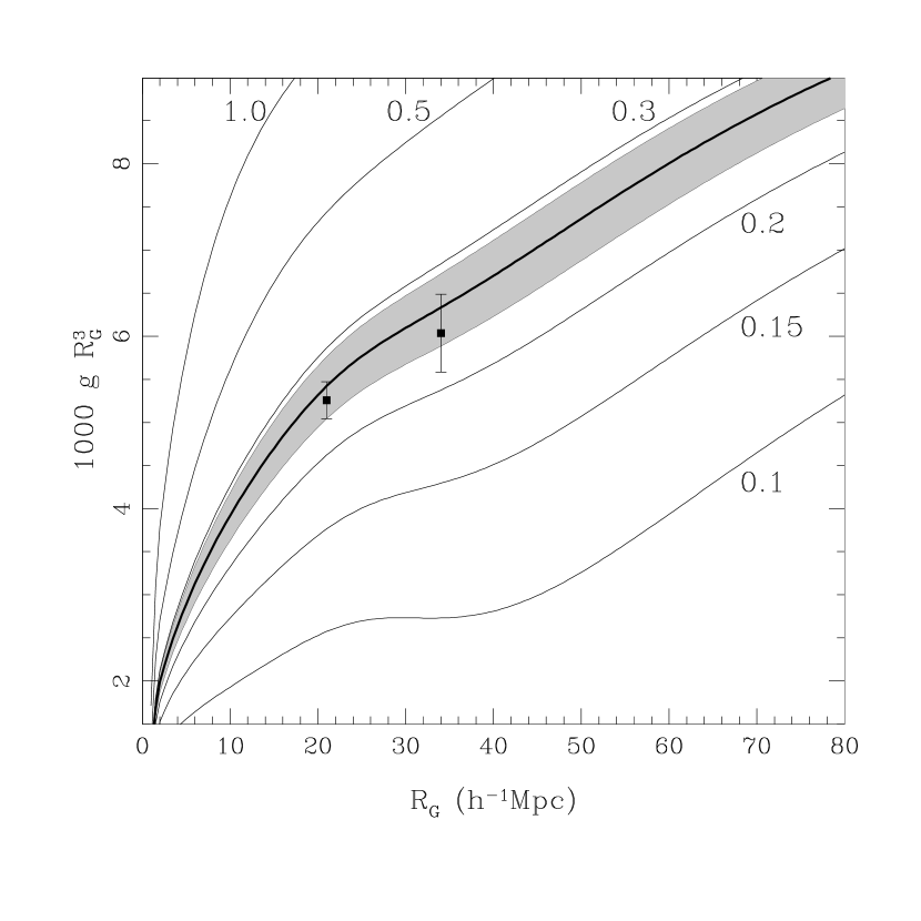
Figure 1.— Amplitude of the genus curve per unit smoothing volume for the flat $\Lambda$CDM models with $\Omega_{m}+\Omega_{\Lambda}=1$. The label on each line is $\Omega_{m}$ and the remaining cosmological parameters are set to those from the WMAP 5-year data. The thick line is for $\Omega_{m}=0.26$, and the boundaries of the shaded region correspond to $\Omega_{m}=0.29$ and 0.23, which are chosen from the mean and the $1\sigma$ uncertainty limits of the WMAP 5-year data. The data points are from the SDSS DR4plus sample (Gott et al. 2009).

Figure 1 shows the amplitude of the genus curve per unit smoothing volume, $gR_{G}^{3}$, when the matter field is smoothed over $R_{G}$ by a Gaussian filter, for a series of the flat $\Lambda$CDM models with $\Omega_{\rm m}+\Omega_{\Lambda}=1$ and $h=0.72$. The label on each curve is the value of $\Omega_{\rm m}$. Each curve has a characteristic shape reflecting the shape of the $\Lambda$CDM PS with different $\Omega_{\rm m}$. A comparison between these curves and $gR_{G}^{3}$ measured from low redshift LSS data constrains the cosmological parameters related with the shape of the PS. The uncertainty in $\Omega_{m}$ from the WMAP 5-year data corresponds to 6.6% variation in the genus amplitude at $R_{G}=20h^{-1}$Mpc, for example (see the shaded region in Fig. 1). The two data points are from Gott et al. (2009) who measured $A$ with 4% uncertainty at 21 $h^{-1}$Mpc using the SDSS DR4plus sample.

3. Expansion History of the Universe

As the universe expands, the cosmic sponge remains unchanged and the shape of the PS at large scales is conserved in the comoving space. If an observational sample of LSS covers a range of redshift, one can measure the PS or CF in different redshift intervals and compare their shapes to check whether or not the adopted $r(z)$ relation is correct. If their shapes in different redshift intervals do not agree with one another, we change the cosmological parameters and thus $r(z)$ relation until an agreement is achieved. In this section we will consider only the Gaussian fluctuation case, where the genus amplitude gives information equivalent to the shape of the PS, for a demonstration of concept.

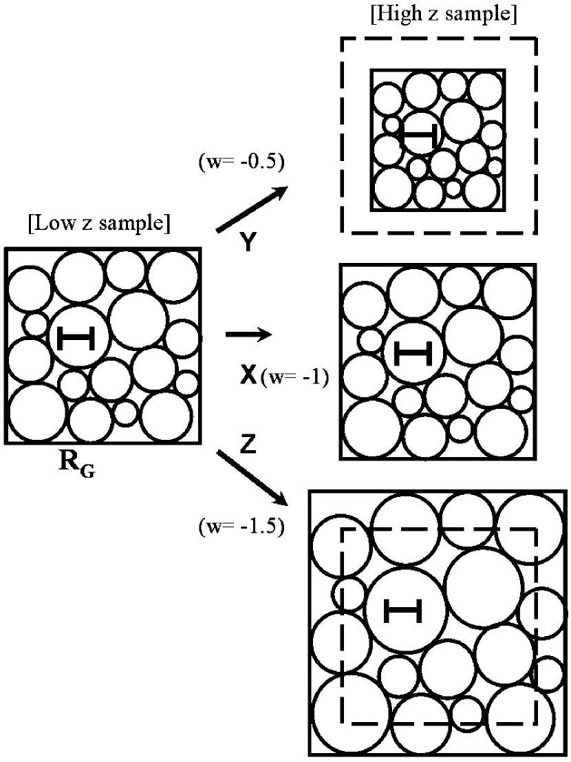
Figure 2.— A schematic diagram illustrating changes in the unit volume (dashed boxes) and smoothing scale (error bars) when different $r(z)$ relations are adopted for large-scale structure data observed at low and high redshifts, supposing the true cosmology is X and the assumed cosmologies are Y and Z with wrong $w$’s.

Figure 2 illustrates what happens to the LSS analysis when wrong $r(z)$ relations (wrong cosmologies) are adopted. Suppose one is trying to constrain $w$ while other parameters are fixed. The box on the left shows LSS at low redshift in a square region of the universe with $w=-1$. The error bar indicates the smoothing scale. If one transforms the redshifts of distant galaxies to comoving distances using the $r(z)$ relation adopting the correct value of $w$, a region having the same comoving size located at high redshift will enclose the same comoving volume and the smoothing length will correspond to the scale equal to that at $z=0$ (the middle box on the right). But if we choose $w=-0.5$, we mistakenly think the space is expanding slower than the reality. As a result of the wrong $r$-$z$ transformation, a unit volume (the dashed box in Fig. 2) will enclose more LSS than the box does at $z=0$, and the smoothing length corresponds to a scale larger than that at low $z$. Because the box of a unit comoving volume contains more LSS but the smoothing is made over a larger scale, their effects on the genus partially cancel with each other but there remains some net effect unless the density fluctuation field is scale-free. When one adopts a universe that expands faster than the real one ($w=-1.5$ for example), the comoving volume of the box at high redshift actually amounts to a smaller volume compared to that in the true cosmology, and the smoothing scale corresponds to a scale smaller than what it is intended to.

The amplitude of the genus curve when a wrong cosmology ‘Y’ is adopted while the true cosmology is ‘X’, can be estimated in the following way. The volume factor at redshift $z$ in a cosmology is given by $V=D_{A}^{2}/H(z)$ (Peebles 1993). When a wrong cosmology is adopted, the fractional change in volume is $V_{X}(z)/V_{Y}(z)$ when the samples are constrained to have the same comoving volume under the given cosmologies. (Due to the Alcock-Paczynski effect, the amount of radial and tangential length variations is slightly different from each other. In the present treatment we average structures over angles and consider only the volume effect.) On the other hand, the smoothing length changes by a factor $\lambda_{XY}(z)=[V_{X}(z)/V_{Y}(z)]^{1/3}$. Therefore, the amplitude of the genus curve measured when the wrong cosmology $Y$ is adopted to convert redshifts to comoving distance, becomes

$$g_{\rm Y}(z;R_{G})=g_{\rm X}(z;R_{G}^{\prime})V_{\rm X}(z)/V_{\rm Y}(z),$$ (2)

where $R_{G}^{\prime}=\lambda_{XY}(z)R_{G}$. This formula is equivalent to $g_{\rm Y}(z;R_{G})R_{G}^{3}=g_{\rm X}(z;R_{G}^{\prime}){R^{\prime}}_{G}^{3}$. Any change in cosmology that affects the expansion history of the universe will result in change in the redshift dependence of $g(R_{G})$. One can use this formula to estimate the genus in a particular cosmology when its value for a fiducial cosmology is known without making full numerical mock sample analysis. Cosmological parameters can be constrained through an iterative process to minimize the difference between observations and the theoretical prediction. In practice, observational data occupy a finite redshift interval, and the scaling factors in Equation (2) should be replaced by an integral over redshift. It should also be pointed out that the number density of the objects tracing the LSS will show a radial gradient due to the redshift dependence of the volume factor when a wrong cosmology is adopted. If the radial distribution of the tracers is forced to be uniform, the selection criterion of the objects will become non-uniform.

When one measures the two-point CF under the assumption of a wrong cosmology $Y$, one will incorrectly scale the separation between galaxies, and the position of features in the CF moves by the scaling factor, namely $\xi_{Y}(s;z)=\xi_{X}(s^{\prime};z)$ where $s^{\prime}=\lambda_{XY}(z)s$ (see also Percival et al. 2007). This causes the slope of the CF to change. Likewise, the PS is scaled as $P_{Y}(k;z)=P_{X}(k^{\prime};z)$ where $k^{\prime}=\lambda_{XY}^{-1}(z)k$.

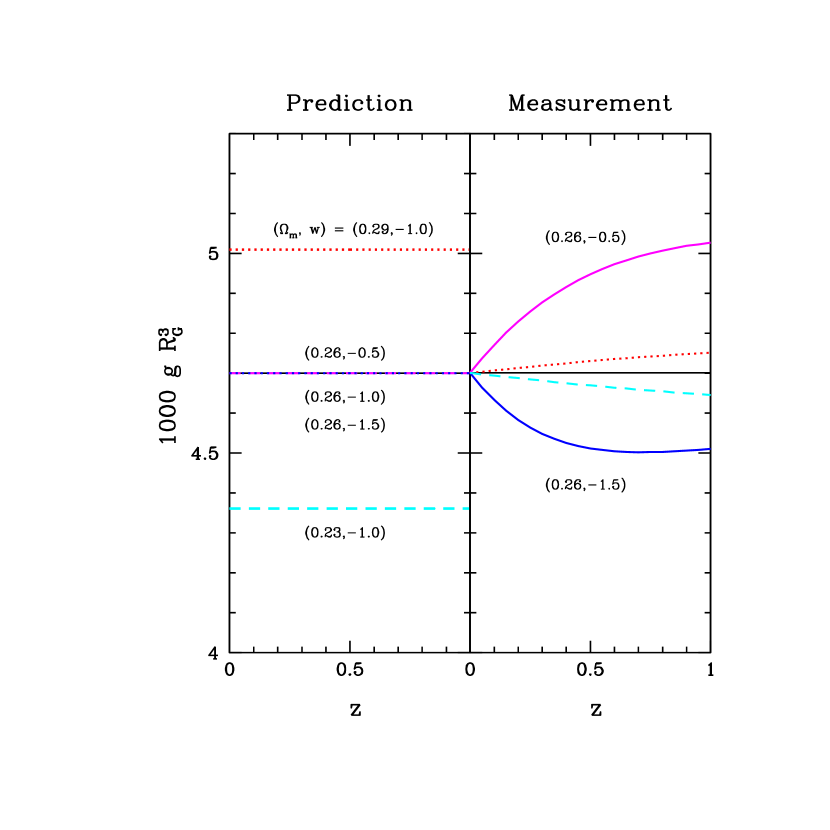
Figure 3.— The genus per unit smoothing volume at $R_{G}=15h^{-1}$Mpc for five flat cosmological models with different sets of $(\Omega_{m},w)$ (left panel). The right panel shows the genus that will be actually measured when five different sets are assumed in the $r$-$z$ transformation even though the correct one is $(0.26,-1.0)$.

Figure 3 shows how the genus is used to measure the cosmological parameters that govern the expansion history of the universe. Here it is again assumed that the true cosmology has $\Omega_{\rm m}=0.26$ and $\Omega_{\rm E}=0.74$ with $w=-1$ (The subscript E stands for the dark energy). We adopt $\Omega_{m}+\Omega_{\rm E}=1$, and all remaining parameters are fixed to the WMAP 5-year parameters. The left panel shows the predicted amplitude of the genus curve at $R_{G}=15\;h^{-1}{\rm Mpc}$ when different sets of ($\Omega_{\rm m},w$) are adopted. Each line is independent of $z$ because the shape of the linear PS is conserved in the comoving space. It is also independent of $w$ since $w$ does not change the shape of the linear PS. The lines in the right panel are the genus per unit smoothing volume that will be measured when five different cosmologies are adopted. It demonstrates that the redshift-dependence of the genus amplitude is quite different for cosmologies with different $\Omega_{m}$ and $w$. The correct choice of (0.26, $-1.0$) will result in an agreement between the theoretical prediction, the horizontal line with $gR^{3}_{G}=0.00470$, and the observationally measured one. But when (0.26, $-0.5$) is mistakenly adopted, the wrong $r(z)$ makes the genus amplitude overestimated. This means the volume factor dominates the change in Equation 2. At $z=0.5$, the measured value will be 5.3% larger than the predicted value. When the fractional error in the observed $g$ is $\Delta_{g}$, the fractional error in $w$ constrained by this single data point is roughly $\Delta_{w}=9.5\Delta_{g}$. Therefore, if the genus is measured with accuracy better than 1% at $z\sim 0.5$, one can constrain $w$ with error less than about $10\%$ by comparing the theoretical prediction with what is actually measured. When a model with more negative $w$ is adopted, the measured genus amplitude falls below the predicted value [see the (0.26, $-1.5$) case].

4. Summary

The key points of this paper can be summarized as follows:

1. We point out that the pattern of the LSS is conserved in time and can be used as a cosmic standard ruler.

2. We propose to use the sponge topology of LSS as a more robust standard ruler than $P(k)$ or $\xi(r)$ because the intrinsic topology statistics are less susceptible to various non-linear systematic effects.

To enhance the power of the standard rulers it is necessary to have accurate knowledge on the systematic effects such as non-linear gravitational evolution, scale-dependent galaxy biasing, and redshift-space distortion (Park, Kim & Gott 2005; James et al. 2009). This will be the subject of our subsequent paper (Kim et al. 2009).

Recently, Gott et al. (2009) measured the genus amplitude with 4% error at the smoothing scale of 21 $h^{-1}$Mpc from the Luminous Red Galaxy sample of the SDSS DR4plus. The current redshift survey sample already reached the size that enables us to do the topology study at a few percent uncertainty level. The final SDSS DR7 data and the future LSS surveys are expected to significantly increase the accuracy. Various constrains on $w$ from existing and future surveys will be presented by Kim et al. (2009)

In addition to the 3D genus, one can also use the scale-dependence of the 1D level-crossing statistic or the 2D genus of LSS as the standard rulers. For example, cosmological parameters can be estimated by requiring the level crossings per unit comoving length in the radial distribution of $Ly$-$\alpha$ forest clouds to be constant in time. The 2D genus of the galaxy distribution in the photometric redshift slices can be also used to constrain the expansion history of the universe. We will explore the usefulness of these statistics in the forthcoming papers.

References

- (1) Alcock, C., & Paczynski, B. 1979, Nature, 281, 358
- (2) Allen, S. W., Schmidt, R. W., Ebeling, H., Fabian, A. C. & van Speybroeck, L., 2004, MNRAS, 353, 457
- (3) Blake, C., & Glazebrook, K. 2003, ApJ, 594, 665
- (4) Bond, J. R., Kofman, L., & Pogosyan, D., 1996, Nature, 380, 603
- (5) Colgate, S., 1979, ApJ, 232, 404
- (6) Cooray, A. R., & Huterer, D. 1999, ApJ, 513, 95
- (7) Corasaniti, P. S., Bassett, B. A., Ungarelli, C., & Copeland, E. J. 2003, Phys.Rev.Lett. 90, 091303
- (8) Doroshkevich, G. 1970, Astrophysika, 6, 320
- (9) Dunkley, J., Komatsu, E., Nolta, M. R., Spergel, D. N., Larson, D., Hinshaw, G., Page, L., Bennett, C. L., et al. 2009, ApJS, 180, 306
- (10) Gott, J. R., Choi, Y.-Y., Park, C., & Kim, J. 2009,ApJ, 695, L45
- (11) Gott, J. R., Melott, A. L., & Dickinson, M. 1986, ApJ, 306, 341
- (12) Hamilton, A. J. S., Gott, J. R., & Weinberg, D. W. 1986, ApJ, 309, 1
- (13) James, J. B., Colless, M., Lewis, G. F., & Peacock, J. A. 2009, MNRAS, 394, 454
- (14) Kim, Y.-R., Park, C., Kim, J., & Gott, J., R., 2009, in preparation
- (15) Maddox, S. J., Sutherland, W. J., Efstathiou, G., & Loveday, J. 1991, in Large-Scale Structures and Peculiar Motions in the Universe, ASP Conference Series, Vol. 15, ed. D. W. Latham, & L. N. da Costa, p. 213
- (16) Meiksin, A., White, M., & Peacock, J. A. 1999, MNRAS, 304, 851
- (17) Park, C., Choi, Y.-Y., Vogeley, M. S., Gott, J. R., Kim, J., Hikage, C., Matsubara, T., Park, M. G., Suto, Y., & Weinberg, D. H. 2005, ApJ, 633, 11
- (18) Park, C., Kim, J., & Gott, J. R. 2005, ApJ, 633, 1
- Peebles (1993) Peebles, P. J. E. 1993, Princeton Series in Physics, Princeton, NJ: Princeton University Press, p332
- (20) Peebles, P. J. E., & Yu, J. T. 1970, ApJ, 162, 815
- (21) Percival, W. J., Cole, S, Eisenstein, D. J., Nicho, R. C., Peacock, J. A., Pope, A. C., & Szalay, A. S., 2007, MNRAS, 381, 1053
- (22) Perlmutter, S., Aldering, G., Goldhaber, G., Knop, R. A., Nugent, P., Castro, P. G., Deustua, S., Fabbro, S., et al., 1999, ApJ, 517, 565
- (23) Rapetti, D., Allen, S. W. & Weller, Jochen, 2005, MNRAS, 360, 555
- (24) Riess, A. G., Filippenko, A. V., Challis, p., Clocchiatti, A., Diercks, A., Garnavich, P. M., Gilliland, R. L., Hogan, C. J, et al. 1998, AJ, 116, 1009
- (25) Sachs, R. K., & Wolfe, A. M., 1967, ApJ, 147, 73
- (26) Tegmark, M., Eisenstein, D. J., Strauss, M. A., Weinberg, D. H., Blanton, M. R., Frieman, J. A., Fukugita, M., Gunn, J. E., et al. 2006, Phys. Rev. D., 74, 123507
- (27) Vogeley, M. S., Park, C., Geller, M. J., Huchra, J. P. & Gott, J. R. 1994, ApJ, 420, 525