The Partonic Nature of Instantons

Abstract:

In both Yang-Mills theories and sigma models, instantons are endowed with degrees of freedom associated to their scale size and orientation. It has long been conjectured that these degrees of freedom have a dual interpretation as the positions of partonic constituents of the instanton. These conjectures are usually framed in $d=3+1$ and $d=1+1$ dimensions respectively where the partons are supposed to be responsible for confinement and other strong coupling phenomena. We revisit this partonic interpretation of instantons in the context of $d=4+1$ and $d=2+1$ dimensions. Here the instantons are particle-like solitons and the theories are non-renormalizable. We present an explicit and calculable model in $d=2+1$ dimensions where the single soliton in the ${\bf CP}^{N}$ sigma-model can be shown to be a multi-particle state whose partons are identified with the ultra-violet degrees of freedom which render the theory well-defined at high energies. We introduce a number of methods which reveal the partons inside the soliton, including deforming the sigma model and a dual version of the Bogomolnyi equations. We conjecture that partons inside Yang-Mills instantons hold the key to understanding the ultra-violet completion of five-dimensional gauge theories.

1 Introduction

Solitons in field theory often have, in addition to their translational degrees of freedom, a number of further collective coordinates that arise from the action of internal symmetries. Two prime examples of this are:

• Solitons in the ${\bf CP}^{N-1}$ sigma-model: The single soliton has two translational modes, a scaling mode and $2N-3$ orientational modes arising from the $SU(N)$ global symmetry. This gives $2N$ collective coordinates in total.

• Yang Mills instantons: The instanton in $SU(N)$ gauge theory has 4 translational modes, a scaling mode and $4N-5$ orientational modes coming from large $SU(N)$ gauge transformations. This gives $4N$ collective coordinates in total.

In both of these cases, all collective coordinates are Goldstone modes arising from the underlying symmetries of the theory. However, it has long been conjectured that, under certain circumstances, there may be a different interpretation for these collective coordinates as the positions of $N$ constituent objects which make up the soliton [2]. (More recent proposals along these lines include [3, 4, 5]). These constituents have been christened with a variety of names over the years, from the mundane “fractional instanton” or “instanton quark” to more flowery “zindon” or “quink”. Throughout this paper, we err on the side of the mundane and refer to the instanton constituents simply as “partons”.

Conjectures about the partonic nature of instantons are usually framed in the context of strongly coupled phenomena in $d=1+1$ dimensions (for sigma-models) and $d=3+1$ dimensions (for Yang-Mills theories). Such discussions typically hinge on the hope that some class of field configurations dominates the path integral, even at strong coupling, resulting in a vacuum which can be understood as a soup of correlated partons.

In this paper we will discuss the role of these partons in $d=2+1$ dimensions (for sigma-models) and $d=4+1$ dimensions (for Yang-Mills theories). In these dimensions, the instanton solutions are particle-like solitons. The theories are weakly coupled in the infra-red, but non-renormalizable and require completion in the ultra-violet (UV). The premise of this paper is that, in some situations, the partons provide the degrees of freedom that form this UV completion.

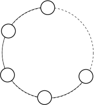
Figure 1:

The main purpose of this paper is to provide a detailed example where the partonic nature of solitons is explicit, and under analytic control. The example that we offer is a supersymmetric gauge theory in $d=2+1$ dimensions which flows, in the infra-red, to a variant of the ${\bf CP}^{N-1}$ sigma-model. The field content of the gauge theory is shown in the quiver diagram: it consists of a $U(1)^{N}$ gauge group, together with $N$ matter fields carrying charge $(+1,-1)$ under consecutive $U(1)$ factors.

The sigma-model of interest arises as the Coulomb branch of this theory. This means that after integrating out the matter multiplets, and dualizing the photons, the low-energy dynamics of the gauge theory is captured by a suitable variant of the ${\bf CP}^{N-1}$ sigma-model [8]. (To be precise, the Coulomb branch is the cotangent bundle $T^{\star}{\bf CP}^{N-1}$).

Although we integrate out the charged matter to arrive at the sigma-model description, we have not lost all trace of it. Its memory remains in the guise of the soliton. A single soliton can be shown to be a multi-particle state, formed from the matter multiplets that have been integrated out. Our goal in this paper is to answer the inverse question: “Given access to the low-energy sigma-model, what can we learn about the UV gauge theory through a study of the soliton?” Surprisingly, we show that the properties of the soliton allows us to reconstruct the microscopic quantum numbers of the partons, details which one would imagine had been swept away by the winds of the renormalization group.

We introduce a number of methods that demonstrate the partonic nature of the sigma-model lumps. Perhaps the cleanest is to study the instantons in a deformation of the sigma-model, in which a single soliton solution decomposes into $N$ constituents and allows us to graphically demonstrate the existence of partons. We further show that the soliton equations can be re-interpreted as the equations of electrically charged point-like sources. In this reformulation, the scale and orientation moduli of the soliton can be explicitly seen to be the positions of $N$ partons carrying the quantum numbers dictated by the microscopic quiver theory. Moreover, this provides insight into the manner in which fundamental fields morph into solitons. Finally, we also describe the relationship between our partons and calorons which arise when the theory is compactified on a circle.

All the work presented in this paper was undertaken with an eye to the harder problem of partons in Yang-Mills instantons. We hope to address this question in a future publication and, for now, limit ourselves only a few relevant observations which form the content of Section 4.

2 Partons in the ${\bf CP}^{1}$ Sigma Model

In this section we discuss solitons in the ${\bf CP}^{1}$ sigma model. We describe several methods which reveal the two partons sitting inside each soliton. All of these methods can be generalized to the ${\bf CP}^{N-1}$ sigma model at the expense of more cumbersome notation which is postponed until Section 3.

We will consider a sigma model with target space $T^{\star}{\bf CP}^{1}$, that is the cotangent bundle of ${\bf CP}^{1}$. This has the same soliton spectrum as ${\bf CP}^{1}$ but admits an extension to a theory with ${\cal N}=4$ supersymmetry. (This means eight supercharges in $d=2+1$ dimensions). The sigma model is non-renormalizable and requires a UV completion. Following [8], we realise this UV completion by constructing the sigma model as the Coulomb branch of a gauge theory. We start by reviewing this construction.

2.1 A UV Completion of the Sigma Model

${\cal N}=4$ theories in $d=2+1$ dimensions have a global $SU(2)_{R}\times SU(2)_{N}$ R-symmetry. The theories we consider in this paper are built from two standard multiplets:

• The vector multiplet contains a gauge field $A_{\mu}$ and three real scalar fields $\!\vec{\,\phi}$ transforming in the $({\bf 1},{\bf 3})$ representation of the R-symmetry group. There are also four Majorana fermions transforming as $({\bf 2},\bar{\bf 2})$.

• The hypermultiplet contains a doublet of complex scalar fields $Q=(q,\tilde{q}^{\dagger})$, transforming as $({\bf 2},{\bf 1})$ under the R-symmetry. The four Majorana fermions transform as $({\bf 1},{\bf 2})$.

Our theory consists of a single $U(1)$ vector multiplet coupled to two hypermultiplets $Q_{1}$ and $Q_{2}$ with charge $+1$ and $-1$ respectively. The bosonic part of the Lagrangian is given by,

$$-{\cal L} = \frac{1}{4e^{2}}F_{\mu\nu}F^{\mu\nu}+\frac{1}{2e^{2}}(\partial_{\mu}\phi)^{2}+\sum_{i=1}^{2}\left(|{\cal D}_{\mu}q_{i}|^{2}+|{\cal D}_{\mu}\tilde{q}_{i}|^{2}\right)$$ (2.1)

$$+(\vec{m}+\!\vec{\,\phi})^{2}(|q_{1}|^{2}+|\tilde{q}_{1}|)^{2}+(\vec{m}-\!\vec{\,\phi})^{2}(|q_{2}|^{2}+|\tilde{q}_{2}|^{2})$$

$$+\frac{e^{2}}{2}(|q_{1}|^{2}-|q_{2}|^{2}-|\tilde{q}_{1}|^{2}+|\tilde{q}_{2}|^{2})^{2}+2e^{2}|\tilde{q}_{1}q_{1}-\tilde{q}_{2}q_{2}|^{2}\ .$$

Here $e^{2}$ is the gauge coupling constant,while $\vec{m}$ is a triplet of mass parameters. The vector multiplet is massless while, for generic values of $\!\vec{\,\phi}$, the hypermultiplets are massive. The theory has a single flavour symmetry, $U(1)_{F}$, under which the hypermultiplets $Q_{1}$ and $Q_{2}$ both have charge $+1$.

We are interested in the low-energy effective action for the vector multiplet. This is best described after first dualizing the photon in favour of a periodic scalar field, $\sigma\in[0,2\pi)$, defined by

$$F_{\mu\nu}=\frac{e^{2}}{2\pi}\,\epsilon_{\mu\nu\rho}\partial^{\rho}\sigma$$ (2.2)

Written in the dual variables the theory has a further global symmetry, usually denoted as $U(1)_{J}$, which acts by shifting $\sigma$. In non-Abelian theories this symmetry is typically broken by instanton effects, but in our Abelian theory it remains exact.

After integrating out the hypermultiplets at one-loop, the low-energy effective action is given by a sigma model on the Coulomb branch [8],

$$-{\cal L}=\frac{1}{2}H(\phi)\,(\partial_{\mu}\!\vec{\,\phi})^{2}+\frac{1}{8\pi^{2}}H(\phi)^{-1}(\partial_{\mu}\sigma+\vec{\omega}\cdot\partial_{\mu}\!\vec{\,\phi})^{2}$$ (2.3)

Here the function $H(\phi)$ can be thought of as the renormalized gauge coupling, receiving contributions from each of the two hypermultiplets

$$H=\frac{1}{e^{2}}+\frac{1}{4\pi|\vec{m}+\!\vec{\,\phi}|}+\frac{1}{4\pi|\vec{m}-\!\vec{\,\phi}|}$$ (2.4)

The factor of $4\pi$ in this expression is usually neglected, but arises from an explicit one-loop computation as shown in [9]. This normalization will prove important later in our discussion. The connection $\vec{\omega}$ in (2.3) is defined by $\vec{\nabla}H=\vec{\nabla}\times\vec{\omega}$.

The one-loop effective action (2.3) defines a sigma-model with a hyperKähler metric on two-centered Taub-NUT space. This hyperKähler structure is required by supersymmetry and is sufficient to ensure that there are no further corrections to the action: the one-loop result is exact [8]. In particular, it holds even in the strong coupling limit $e^{2}\rightarrow\infty$. Here something special happens: the $U(1)_{J}$ isometry is enhanced to $SU(2)_{J}$ and the metric (2.3) becomes the Eguchi-Hanson metric on $T^{\star}{\bf CP}^{1}$ [10].

The ${\bf CP}^{1}$ submanifold

We will be interested in the ${\bf CP}^{1}$ submanifold that is the zero section of $T^{\star}{\bf CP}^{1}$. It is also sometimes known as the “bolt”. To define it, we choose for simplicity $\vec{m}=(0,0,m)$. The bolt is then defined as the submanifold with $\!\vec{\,\phi}=(0,0,\phi)$ and $\phi\in[-m,m]$. The metric on the bolt is given by

$$ds^{2}=H(\phi)\,d\phi^{2}+\frac{1}{4\pi^{2}}H(\phi)^{-1}\,d\sigma^{2}$$

with

$$H(\phi)=\frac{1}{e^{2}}+\frac{m}{2\pi(m^{2}-\phi^{2})}$$ (2.5)

For finite $e^{2}$, this is the metric on a squashed sphere written in “toric” coordinates. When $e^{2}\rightarrow\infty$, it becomes the metric on the round sphere with $SU(2)_{J}$ isometry. To see this explicitly, we define the complex coordinate on the Riemann sphere,

$$R=\sqrt{\frac{m-\phi}{m+\phi}}\,e^{i\sigma}$$ (2.6)

in terms of which the metric, in the $e^{2}\rightarrow\infty$ limit, takes the familiar form,

$$ds^{2}=\frac{2m}{\pi}\frac{dR\,d\bar{R}}{(1+|R|^{2})^{2}}$$ (2.7)

2.2 Solitons and Their Microscopic Interpretation

The low-energy sigma model has solitons. These solitons are BPS only if we take the vacuum to lie on the ${\bf CP}^{1}$ bolt defined above. (In fact, if this is not the case, the soliton profile does not have a well-defined asymptotic limit). In this section we study the properties of the soliton and identify this object in the microscopic gauge theory.

Let us first determine the mass of the soliton. It is related to the size of the ${\bf CP}^{1}$ (and this is the reason that the factor of $1/4\pi$ was important in (2.4)). It is a simple matter to write down the lump equations in terms of the $\phi$ and $\sigma$ fields. The energy functional for static configurations can be written as:

$${\cal E} = \int d^{2}x\ \frac{1}{2}H\,\partial_{\alpha}\phi\partial_{\alpha}\phi+\frac{1}{8\pi^{2}}H^{-1}\partial_{\alpha}\sigma\partial_{\alpha}\sigma$$ (2.8)

$$= \int d^{2}x\ \frac{1}{8\pi^{2}}H^{-1}(2\pi H\,\partial_{\alpha}\phi\mp\epsilon_{\alpha\beta}\partial_{\beta}\sigma)^{2}\pm\frac{1}{2\pi}\epsilon_{\alpha\beta}\partial_{\alpha}\phi\partial_{\beta}\sigma.$$

The Bogomolnyi equations can be found sitting within the total square: they are

$$2\pi H(\phi)\,\partial_{\alpha}\phi=\epsilon_{\alpha\beta}\,\partial_{\beta}\sigma$$ (2.9)

where the function $H(\phi)$ is given in (2.5). When these equations are satisfied, the energy is given by the last term in (2.8) which we recognize as the topological charge. It counts the winding of the configuration, weighted by the area of the (squashed) sphere. Recalling that $\phi\in[-m,m]$ and $\sigma\in[0,2\pi)$, this area is given by $4\pi m$. The mass of the BPS lump, given by the lowest energy configuration with unit winding number, is

$$M_{\rm lump}=2m$$

So what is this object in the microscopic gauge theory? We’re looking for a BPS state with mass $2m$. There is only one candidate: the soliton corresponds to a two particle state $Q_{1}Q_{2}$ constructed from the hypermultiplets. This state is neutral under the $U(1)$ gauge symmetry, but charged under the $U(1)_{F}$ flavour symmetry. The flavour charge has morphed into the topological charge at low energies.

The soliton is BPS only for vacua that lie on the ${\bf CP}^{1}$ bolt. But this is also true of the state $Q_{1}Q_{2}$: the requirement that it is BPS is that the two mass-vectors $\vec{m}\pm\!\vec{\,\phi}$ are parallel. This holds when $\!\vec{\,\phi}$ and $\vec{m}$ lie parallel, with $|\!\vec{\,\phi}|\leq|\vec{m}|$. At low energies this descends to the requirement that we lie on the bolt.

This is quite cute. We integrated out the hypermultiplets and might have expected that we’d lost them for good. But, in fact, they re-appear in the low-energy effective action as solitons. It is somewhat reminiscent of the manner in which baryons appear as skyrmions in the chiral Lagrangian. The identification of the soliton with a multi-particle state was first made in the context of mirror symmetry as particle/vortex duality [11] and was elaborated upon further in [12, 13]. In the rest of this section, we will study the implications of this identification in more detail.

The first question that we should answer is: why are the partons bound to form pairs within the soliton? The reason is that, in three dimensions, the $1/r$ fall-off of the electric field ensures that any state charged under a local current has logarithmically divergent mass. There is a similar IR divergence from the massless $\phi$ field. This means that on the Coulomb branch, where the gauge symmetry is unbroken, all finite mass states are associated to gauge invariant operators. In our theory the only such BPS operator is the dipole $Q_{1}Q_{2}$.

Although the infra-red divergence requires that the partons are bound together, there is no static force between them. This is manifested in the solitonic description by the existence of four collective coordinates. Two simply give the center of mass of the soliton, $Z$. The remaining two correspond to a scale size $\rho$ and an orientation collective coordinate $\theta$. In the limit $e^{2}\rightarrow\infty$, where the target space becomes the round sphere, $\theta$ is a Goldstone mode arising from the action of $U(1)_{J}^{\prime}\subset SU(2)_{J}$ on the soliton. This $U(1)_{J}^{\prime}$ is defined by the requirement that it leaves the vacuum invariant and, in general, does not coincide with $U(1)_{J}$. (We will explain an exception to this statement below). As we will describe in detail, when $e^{2}$ is finite and the target space sphere is squashed, $\theta$ is not in general associated with a Goldstone mode.

2.3 How to Tell if Your Soliton Contains Partons

The microscopic interpretation of the soliton is as a dipole of charged hypermultiplets. We would like to ask what memory the soliton has of its microscopic origins. In other words, suppose that we have access only to low-energy information captured within the sigma model: what would we be able to say about the hypermultiplets that we have integrated out? Here we offer a number of methods which reveal the partonic nature of the soliton. Throughout this section we work in the vacuum $\langle\phi\rangle=0$ where the two partons have equal mass $m$. (We will relax this condition in Section 2.4).

2.3.1 Deforming the Sigma Model

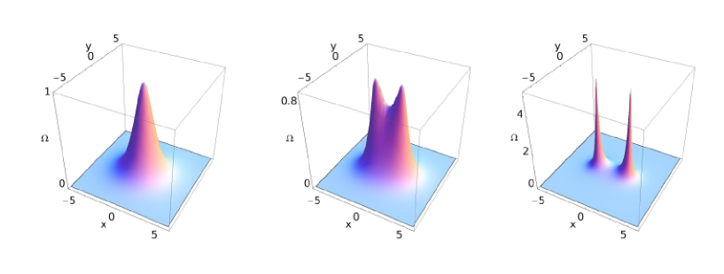
Figure 2: Energy density for a single BPS soliton in ${\bf CP}^{1}$ with $m/e^{2}=0$, $1/2$, $3/2$.

The simplest and most explicit method which reveals the partons is to look at the single soliton solution in the deformed ${\bf CP}^{1}$ sigma-model. The deformation that we have in mind occurs naturally in our UV theory: it is the squashed target space with $H(\phi)$ given by (2.5) with finite $e^{2}$.

When $m/e^{2}=0$, and the target space inherits the round metric, a plot of the energy density reveals no hint of the microscopic structure. It simply gives a blurred lump of size $\rho$ as shown in the first plot of Figure 2. The remaining two plots in the figure show the energy density of the BPS soliton as $m/e^{2}$ increases and the target space is squashed into the shape of a rugby ball. The topological charge becomes localized around the tips at $\phi=\pm m$. In space, we see that the energy density becomes localized in two equal peaks, each with ${\cal E}=m$, sitting at positions $z_{+}$ and $z_{-}$, separated by a distance $|z_{+}-z_{-}|=2\rho$.

In the limit $m/e^{2}\rightarrow\infty$, the parton configuration in the figure is reminiscent of the “meron” configuration described in [14]. A single parton has topological charge $1/2$, as does a single meron. However, there are also differences. Our configuration is a solution to the equations of motion on the squashed sphere; the meron configuration is a singular solution to equations on the round sphere. This difference becomes most manifest when we look to generalize the discussion to the ${\bf CP}^{N-1}$ sigma-model. The meron continues to have topological change $1/2$ in this context while, as we will see in the following section, deforming the metric on ${\bf CP}^{N-1}$ causes the lump to decompose into $N$ partons with topological charge $1/N$. A similar mechanism for revealing the partonic structure of sigma-model lumps was independently found in [15].

2.3.2 Parton Quantum Numbers

We saw above that deforming the sigma model target space dramatically reveals the partonic nature of the soliton. But suppose that we work in the $e^{2}\rightarrow\infty$ limit where the target space is round and the energy density is merely a smeared blob. Is it still possible to disentangle the partonic structure? The answer, as we shall see, is yes.

The first hint at a partonic structure was described long ago in [2] and arises from simply looking at the solution in different variables. In the $e^{2}\rightarrow\infty$ limit, the profile of a single soliton is given by

$$\phi=m\rho\,\frac{e^{-i\theta}(z-Z)+e^{i\theta}(\bar{z}-\bar{Z})}{|z-Z|^{2}+\rho^{2}}$$

The four collective coordinates of the solution are $Z\in{\bf C}$, the centre of mass, $\rho\in{\bf R}^{+}$, the scale size of the soliton, and $\theta\in[0,2\pi)$, a Goldstone mode arising from the $U(1)^{\prime}_{J}\subset SU(2)_{J}$ flavour symmetry which is left unbroken by the choice of vacuum.

However the fact that the collective coordinates can be re-interpreted as the positions of partons is clear if we rewrite the soliton solution using the coordinate $R$ on target space, defined in (2.6). Then the single soliton solution takes the form,

$$R=\frac{z-z_{+}}{z-z_{-}}$$ (2.10)

with $Z={\textstyle\frac{1}{2}}(z_{-}+z_{+})$ and $\rho e^{i\theta}={\textstyle\frac{1}{2}}(z_{-}-z_{+})$. The collective coordinates $z_{+}$ and $z_{-}$ reveal the positions of the partons. Indeed, at $z=z_{\pm}$ we have $\phi=\pm m$, so at each of these locations one of the hypermultiplets of our microscopic theory becomes massless. We will shortly see that the soliton profile near these points reveals that the configuration carries the correct electric charge.

There is a simple generalization of the single soliton solution (2.10) to a $k$ soliton solution,

$$R=\prod_{n=1}^{k}\frac{z-z_{+}^{n}}{z-z_{-}^{n}}$$ (2.11)

where $\{z_{+}^{n}\}$ and $\{z_{-}^{n}\}$ denote the positions of the hypermultiplet excitations $Q_{1}$ and $Q_{2}$ respectively. The fact that the $k$-lump solution is determined by the positions of two sets of $k$ points on the plane has long been taken as evidence for the partonic nature of the soliton [2]. This fact is explicitly realised in the three dimensional gauge theory construction.

Dual Bogomolnyi Equations

The partons $Q_{1}$ and $Q_{2}$ in the microscopic model carry electric charge $\pm 1$ under the $U(1)$ gauge field. They also carry flavour charge $+1$ under $U(1)_{F}$. This flavor symmetry descends to the topological charge of the sigma model. But it is also possible to reconstruct the electric charge of the partons from the lump solutions.

To do this, we rewrite the soliton equations (2.9) in terms of dual variables. We begin by inverting the duality transformation (2.2), this time with the low-energy gauge field $F_{\mu\nu}$ defined in terms of the renormalized gauge coupling,

$$F_{\mu\nu}=\frac{H^{-1}}{2\pi}\,\epsilon_{\mu\nu\rho}\partial^{\rho}\sigma$$ (2.12)

In these variables, the Bogomolnyi equation (2.9) simply relates the electric field to the variation of $\phi$,

$$\partial_{\alpha}\phi=F_{0\alpha}$$ (2.13)

Although these equations are merely a re-writing of the Bogomolnyi equations, they do not have smooth solutions corresponding to solitons. Instead, in order to reproduce the soliton profiles, we must introduce point-like sources. This is to be expected in an electrical formulation of the theory.

The transformation (2.12) ensures that the electric field is divergence free except at points where $\sigma$ is ill-defined. It is simple to see where these points lie from the expressions (2.6) and (2.11): they are at $z=z_{+}^{n}$ and $z=z_{-}^{n}$. Since $\sigma$ has non-trivial winding around each of these points, they act as sources for the electric field. In particular, we note from (2.11) that $\sigma$ increases by $2\pi$ if we complete an anticlockwise circuit around $z_{+}^{n}$, and $\sigma$ decreases by $2\pi$ if we complete an anticlockwise circuit around $z_{-}^{n}$. Hence for an arbitrary closed loop $\mathcal{C}$ which avoids the points $z_{\pm}^{n}$ and encloses a region $\mathcal{S}$, we have

$$\int_{\mathcal{C}}dx_{\alpha}\ \partial_{\alpha}\sigma=2\pi\int_{\mathcal{S}}dS\ \sum_{n}\left[\delta(z-z^{n}_{+})-\delta(z-z^{n}_{-})\right]$$ (2.14)

We can rewrite the left-hand-side of this equation using Stokes’ theorem and the duality (2.12). Since the resulting equation holds for arbitrary regions $\mathcal{S}$, we can equate the integrands to find,

$$\partial_{\alpha}(HF_{0\alpha})=\sum_{n}\ \left[\delta(z-z^{n}_{+})-\delta(z-z^{n}_{-})\right].$$ (2.15)

This is a rather novel method of viewing soliton collective coordinates as sources. For each value of $\{z^{n}_{+}\}$ and $\{z^{n}_{-}\}$, there is a unique solution to (2.13) and (2.15). This determines a point on the soliton moduli space. Typically, the electrically charged particles in a theory arise as fundamental excitations, while magnetically charged objects are associated to solitons. This simple model in three dimensions provides an example where we can swap between these two descriptions with ease.

2.3.3 The Force Between Solitons

The dual Bogomolnyi equations above reveal that the partons carry electric charge, and we already mentioned that this is responsible for the logarithmic confinement of the partons with the soliton. Although there is no static force between the partons, the logarithmic infra-red divergence suffered by any individual parton reappears once we ask them to move. It is well known that the moduli space metric for sigma-model lumps has logarithmic infra-red divergences [17]. For ${\bf CP}^{1}$ lumps, there is just a single divergent mode that arises from the long-range tail of $R$,

$$\dot{R}\sim\sum_{n}\frac{\dot{z}_{+}^{n}-\dot{z}_{-}^{n}}{z}+\ldots$$

The kinetic terms are finite only if the sum $\sum_{n}(z_{+}^{n}-z_{-}^{n})$ is constant. This is precisely the condition that the sum of the dipole moments is unchanged, as expected from the microscopic theory.

While solitons have only velocity-dependent forces, there is an attractive force between a lump and an anti-lump. This calculation was performed many years ago and provides yet another method to illuminate the partonic structure of the soliton [14]. One starts by constructing a configuration describing a well-separated lump and anti-lump. The lump has size $\rho$ and orientation $\theta$ and is placed at the origin. The anti-lump has size $\bar{\rho}$ and orientation $\bar{\theta}$ and centre of mass position $z=re^{i\chi}$, where $r\gg\rho,\bar{\rho}$. The interaction energy between the two objects is then computed to be [14]

Figure 3:

$$V_{\rm int}=-4m\,\frac{\rho\bar{\rho}}{r^{2}}\,\cos\left(\theta+\bar{\theta}-2\chi\right)$$

This is precisely the interaction energy of two dipoles on the plane, with orientation $\rho e^{i\theta}$ and $\bar{\rho}e^{i\bar{\theta}}$, separated by $re^{i\chi}$. Indeed, it can be put in slightly more familiar form if we define $\vec{\rho}_{1}=\rho(\cos\theta,\sin\theta)$, $\vec{\rho}_{2}=\bar{\rho}(\cos\bar{\theta},\sin\bar{\theta})$ and $\vec{r}=r(\cos\chi,\sin\chi)$. Then the interaction potential can be written as the dipole interaction,

$$V_{\rm int}=-\frac{4m}{r^{2}}\left(2(\vec{\rho}_{1}\cdot\hat{\vec{r}})(\vec{\rho}_{2}\cdot\hat{\vec{r}})-\vec{\rho}_{1}\cdot\vec{\rho}_{2}\right)$$

It is remarkable that this inter-soliton force captures the partonic structure in such a clean fashion.

Finally, it’s worth mentioning another famous calculation which, while not directly relevant to the present discussion, also reveals the partonic nature of instantons in the ${\bf CP}^{1}$ sigma-model. This is the computation of the determinants around the background of multiple lumps for the theory in $d=1+1$ dimensions [18, 19]. This computation reveals a dipole-like structure for these objects even when viewed as instantons localized in Euclidean spacetime.

2.4 Relationship to Calorons

There is another context in which it is known that the sigma-model lump decomposes into partons, known as calorons. To achieve this, one compactifies the theory on a spatial circle of radius $L$. After deforming the theory in a suitable manner (to be described below), the lump in the ${\bf CP}^{N-1}$ sigma-model can be shown to decompose into $N$ domain walls [20]. (This phenomenon was further discussed in [21] and recently rediscovered in [22, 23, 24]). Importantly, a similar phenomena also occurs for Yang-Mills instantons compactified on a circle [25, 26]. For this reason, we spend some time in this section describing this phenomenon in our sigma model and examining the relationship between the calorons and the partons.

Changing the Vacuum

Until now, we studied the solitons around the vacuum $\langle\phi\rangle=0$. From the perspective of the UV gauge theory, this ensures that the partons have equal bare mass, $m$. In order to understand the relationship to calorons, we will first look at the behaviour of the solitons as we change the vacuum.

As we vary the vacuum, the microscopic masses of the partons change: they become $m\pm\langle\phi\rangle$. The energy density for a single ${\bf CP}^{1}$ soliton is shown in Figure 4 as we vary the vacuum. It is clear that the energy in each spike changes, although the difference in the heights of the spike is not linear in $\langle\phi\rangle$ as one might naively expect from the classical theory. It appears that much of the energy density is dispersed in the field between the solitons. It may be interesting to explore this further, although we shall not do so here.

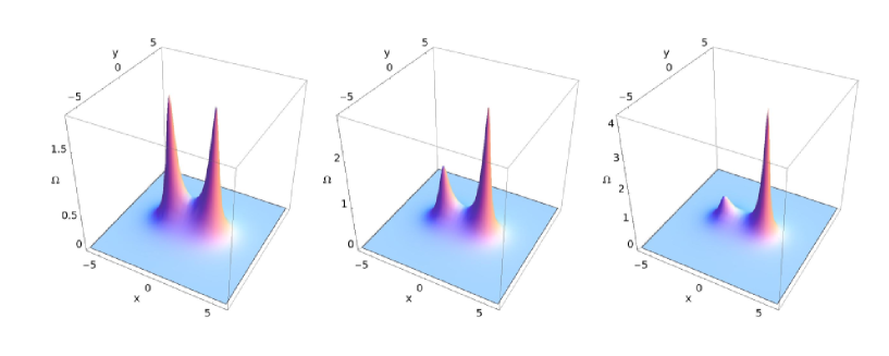
Figure 4: A single ${\bf CP}^{1}$ soliton with $m/e^{2}=1$ as the vacuum varies from $\langle{\phi}\rangle=0$ to $\langle\phi\rangle=0.1m$ to $\langle\phi\rangle=0.2m$.

There is one key feature that will be important in what follows. As $\langle\phi\rangle\rightarrow\pm m$, only a single energy spike survives. In this limit, one of the hypermultiplets in the microscopic theory becomes massless. It is notable that the low-energy dynamics doesn’t notice this fact. Typically, low-energy effective theories become singular when further fields become massless. The reason that this doesn’t happen in three dimensions is due to the infinite energy contained in the long range electric field that accompanies any charged state. This ensures that even though the mass in the Lagrangian vanishes, there are no extra massless charged excitations.

In the context of the soliton, we learn that the partonic description is really not an accurate reflection of the physics when $\langle\phi\rangle=\pm m$. Instead, varying the scale size $\rho$, and the orientation $\theta$ of the lump in the deformed sigma-model does exactly what it says on the tin: it changes the scale size and orientation. Microscopically the scale size arises from exciting a cloud associated to the massless fields. Moreover, in this limit the orientation mode $\theta$ is a Goldstone boson. This is because the symmetry $U(1)_{J}^{\prime}$ that preserves the vacuum coincides with $U(1)_{J}$ and acts on the soliton even when $m/e^{2}\neq 0$.

Introducing a Potential

Before we move on to describe the calorons in this model, it is useful to first recollect what happens when we introduce a potential in the low-energy dynamics. This can be induced in the microscopic theory by a Fayet-Iliopoulos parameter, $\zeta>0$, after which the potential terms in (2.1) become

$$V = (\vec{m}+\!\vec{\,\phi})^{2}(|q_{1}|^{2}+|\tilde{q}_{1}|)^{2}+(\vec{m}-\!\vec{\,\phi})^{2}(|q_{2}|^{2}+|\tilde{q}_{2}|^{2})$$ (2.16)

$$+\frac{e^{2}}{2}(|q_{1}|^{2}-|q_{2}|^{2}-|\tilde{q}_{1}|^{2}+|\tilde{q}_{2}|^{2}-\zeta)^{2}+2e^{2}|\tilde{q}_{1}q_{1}-\tilde{q}_{2}q_{2}|^{2}\ .$$

This theory no longer has a moduli space of vacua, but rather two isolated vacua given by $\vec{\phi}=-\vec{m}$, $|{q}_{1}|^{2}=\zeta$ and $\vec{\phi}=+\vec{m}$, $|\tilde{q}_{2}|^{2}=\zeta$. Upon integrating out the hypermultiplets, this is reflected in our low-energy description on the Coulomb branch (which is now strictly valid only for $m\gg\zeta$) by the presence of the potential,

$$V=\frac{1}{2}\zeta^{2}H(\phi)^{-1}$$ (2.17)

The minima of this potential lie at $\phi=\pm m$. As described above, before we turned on this potential, the partonic interpretation of the soliton was already rather different in these vacua. After turning on the potential, the effect on the soliton is even more dramatic: it shrinks to the singular solution with vanishing scale size $\rho=0$. This behaviour can be understood from the microscopic theory. As can be seen from (2.16), the presence of the FI parameter causes the massless hypermultiplet to condense in the vacuum. This screens the massless cloud which provided the non-zero size $\rho$ of the soliton.

Calorons

We are now in a position to describe the emergence of calorons. We first compactify the spatial direction $x^{2}$ on a circle of radius $L$. The reduced Lorentz symmetry allows for the addition of one further interaction: a theta term $(\theta/4\pi^{2}L)F_{01}$. The theta angle sits in a supermultiplet with the FI parameter $\zeta$ and, as we now explain, induces a potential similar to (2.17). Dualizing the photon in the presence of the theta term means that (2.2) becomes $(2\pi/e^{2})F_{\mu\nu}=\epsilon_{\mu\nu\rho}\partial^{\rho}\sigma-(\theta/2\pi)\epsilon_{\mu\nu 2}$ and the kinetic terms for the dual photon are given by

$$\frac{e^{2}}{8\pi^{2}}\left(\partial_{0}\sigma^{2}-\partial_{1}\sigma^{2}-(\partial_{2}\sigma-\theta/2\pi L)^{2}\right)$$

Upon integrating out the hypermultiplets, $e^{2}$ is again renormalized by $H^{-1}(\phi)$ given in (2.4). The $\theta$ term in the action is then seen to generate a potential term. The effect of the $\theta$ term can be mitigated if $\sigma$ winds $n\in{\bf Z}$ times around the compact circle, so the potential is given by

$$V=\left(\frac{\theta}{2\pi}-n\right)^{2}\frac{H^{-1}(\phi)}{8\pi^{2}L^{2}}$$

The minima are again at $\phi=\pm m$. The physics here is similar to that of the FI parameter. The $\theta$ angle induces a background electric field in two dimensions [27]. This can be screened by a condensation of charged scalars which can only occur at $\phi=\pm m$ where these scalars are massless.

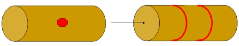
Figure 5: A cartoon of calorons. As the lump grows, it splits into two domain walls.

The isolated vacua in our theory guarantee the presence of domain walls. These are BPS and satisfy the Bogomolnyi equation

$$2\pi H(\phi)\,\partial_{1}\phi=\partial_{2}\sigma-\theta$$ (2.18)

Typically, supersymmetric theories with two vacua have a domain wall which is BPS and interpolates from, say, the first vacuum to the second. If we wish to go back the other way, from the second vacuum to the first, the domain wall is anti-BPS. However, in the present situation both of these walls can be BPS [20, 22]. This is achieved by allowing $\sigma$ to vary along the circle, so that the right-hand side of (2.18) is $>0$ for the first wall, but $<0$ for the second. The reason that these two walls don’t annihilate each other is because the whole configuration carries the topological charge of the lump.

These two domain walls form the calorons of the ${\bf CP}^{1}$ sigma model [20, 22]. In the presence of the $\theta$ term, the lump solution decomposes into two domain wall strings as shown in the figure. This process is entirely analogous to the caloron-monopoles appearing in Yang-Mills theories [25, 26]. For the ${\bf CP}^{N-1}$ sigma-model, the lump decomposes into $N$ calorons.

The above discussion reveals how calorons are related to the hypermultiplet partons of the microscopic theory. Clearly they are not the same objects: the calorons are strings on ${\bf R}^{2}\times{\bf S}^{1}$, while the hypermultiplets are point-like excitations. Instead, the partons share a greater kinship with the individual vacua rather than the domain walls since, in each vacuum, a different hypermultiplet has condensed.

3 Partons in the ${\bf CP}^{N-1}$ Sigma Model

In this section we describe the $N$ partons which lie inside the soliton in the ${\bf CP}^{N-1}$ sigma model. We will find that once again we can recover much of the lost information about the UV degrees of freedom through a careful study of the soliton. We start by describing the UV completion of the sigma model.

3.1 A Quiver Gauge Theory

Figure 6:

We will construct the ${\bf CP}^{N-1}$ sigma model as the Coulomb branch of the quiver gauge theory shown in the figure. This gauge theory has $U(1)^{N}$ gauge group with $N$ hypermultiplets, $Q_{i}$, $i=1,\ldots,N$. The $i^{\rm th}$ hypermultiplet has charge $(+1,-1)$ under $U(1)_{i}\times U(1)_{i+1}$, where we identify $U(1)_{N+1}\equiv U(1)_{1}$. For simplicity, we choose to assign each gauge group the same coupling constant $e^{2}$. The overall diagonal $U(1)\in U(1)^{N}$ is free. Once this is removed, the $N=2$ theory coincides with that described in Section 2.

The theory has a single global symmetry $U(1)_{F}$, under which each hypermultiplet has charge $+1$. By weakly gauging this symmetry, we can introduce a triplet of mass parameters, $\vec{m}$, for the hypermultiplets. These also get masses from their coupling to vector multiplets, so the final mass for the $i^{\rm th}$ multiplet is given by $|\vec{M}_{i}|$, where

$$\vec{M}_{i}=\vec{m}+\!\vec{\,\phi}_{i}-\!\vec{\,\phi}_{i-1}$$ (3.19)

The vector multiplet fields are massless and the low-energy effective action is given by a sigma model on the Coulomb branch, parameterized by the expectation values of $\!\vec{\,\phi}_{i}$ and $\sigma_{i}$, the latter being the dual photons defined in (2.2). Classically, the Coulomb branch is $({\bf R}^{3}\times{\bf S}^{1})^{N}$. The classical metric on the Coulomb branch is inherited from the canonical kinetic terms of the vector multiplet fields. After integrating out the hypermultiplets, the metric receives a correction at one-loop [8] and is given by

$$ds^{2}=H_{ij}\,d\!\vec{\,\phi}_{i}\cdot d\!\vec{\,\phi}_{j}+\frac{1}{4\pi}\,H^{-1}_{ij}\,(d\sigma_{i}+\vec{\omega}_{ik}\cdot d\!\vec{\,\phi}_{k})\,(d\sigma_{j}+\vec{\omega}_{jl}\cdot d\vec{\phi}_{l})$$ (3.20)

This is a multi-dimensional version of the Taub-NUT metric. The matrix $H_{ij}$ has components

$$H_{ii} = \frac{1}{e^{2}}+\frac{1}{4\pi|\vec{M}_{i}|}+\frac{1}{4\pi|\vec{M}_{i+1}|}$$ (3.21)

$$H_{ij} = -\frac{1}{4\pi|\vec{M}_{i}|}\,\delta_{j,i-1}-\frac{1}{4\pi|\vec{M}_{i+1}|}\,\delta_{j,i+1}\ \ \ \ \ i\neq j$$

The connection $\vec{\omega}_{ij}$ obeys $\vec{\nabla}_{i}H_{ij}=\vec{\nabla}_{i}\times\vec{\omega}_{ij}$. As in Section 2, non-renormalization theorems ensure that this one-loop result is the exact description of the low-energy dynamics. Up to discrete identifications, the metric (3.20) has the product form,

$${\cal R}^{3}\times{\bf S}^{1}\times{\cal M}$$

reflecting the fact that the overall, diagonal vector multiplet is decoupled. The metric on ${\cal M}$ is hyperKähler, and closely related to the Lee-Weinberg-Yi metric for monopoles in higher rank gauge groups [28].

The metric on ${\cal M}$ has a $U(1)_{J}^{N-1}$ isometry, arising from shifts in the dual photons $\sigma^{i}$. In the strong coupling limit $e^{2}\rightarrow\infty$, the isometry group is enhanced to $SU(N)$. The metric on ${\cal M}$ becomes the hyperKähler metric on $T^{\star}{\bf CP}^{N-1}$, the cotangent bundle of ${\bf CP}^{N-1}$.

Finding the ${\bf CP}^{N-1}$ Submanifold

Our interest is in the solitons supported by the sigma model on ${\cal M}$. These are BPS objects only if the vacuum state lies on the zero section of $T^{\star}{\bf CP}^{N-1}$, which we will again refer to as the “bolt”. We now describe the bolt in more detail.

We take the bare mass parameter in the metric to lie along $\vec{m}=(m,0,0)$ with $m>0$. The bolt sits within the submanifold in which $\!\vec{\,\phi}_{i}=(\phi_{i},0,0)$. The masses (3.19) then take the form $\vec{M}_{i}=(M_{i},0,0)$ with

$$M_{i}=m+\phi_{i}-\phi_{i-1}$$

The requirement that we lie on the bolt is simply $M_{i}>0$.

Our next goal is to remove the overall free motion, parameterized by $\sum_{i}\phi_{i}$ and $\sum_{i}\sigma_{i}$, leaving only the $2(N-1)$ interacting fields. To this end, we define

$$\hat{\phi}_{J}=\phi_{J}-\phi_{N}-\left(\frac{N}{2}-J\right)m\ \ \ \ \ \ \ J=1,\ldots,N-1$$ (3.22)

There is a similar transformation for the $\sigma_{i}$ variables. It is best described by first introducing the relative field strengths,

$$\hat{F}_{\mu\nu}^{J}=F_{\mu\nu}^{J}-F_{\mu\nu}^{N}\ \ \ \ \ \ \ J=1,\ldots,N-1$$ (3.23)

The $\hat{\sigma}^{I}$ fields are then defined as the dual variables

$$2\pi\hat{H}_{IJ}\hat{F}_{\mu\nu}^{I}=\epsilon_{\mu\nu\rho}\partial_{\rho}\hat{\sigma}_{I}$$ (3.24)

In the variables $\hat{\phi}_{I}$ and $\hat{\sigma}_{I}$, the metric on the bolt can be written as

$$ds^{2}=\hat{H}_{IJ}\,d\hat{\phi}_{I}d\hat{\phi}_{J}+\frac{1}{4\pi}\hat{H}^{-1}_{IJ}\,d\hat{\sigma}_{I}d\hat{\sigma}_{J}$$ (3.25)

with $I,J=1,\ldots N-1$ and the components of $\hat{H}_{IJ}$ given by

$$\hat{H}_{II} = \frac{N-1}{e^{2}N}+\frac{1}{4\pi M_{I}}+\frac{1}{4\pi M_{I+1}}$$

$$\hat{H}_{IJ} = -\frac{1}{e^{2}N}-\frac{1}{4\pi M_{I+1}}\,\delta_{J,I+1}-\frac{1}{4\pi M_{I}}\,\delta_{J,I-1}$$ (3.26)

where this notation means that each non-diagonal element of the matrix $\hat{H}$ contains the constant piece $1/e^{2}N$. The masses, $M_{I}$, now read

$$M_{1} = \hat{\phi}_{1}+\frac{Nm}{2}$$

$$M_{J} = \hat{\phi}_{J}-\hat{\phi}_{J-1}\ \ \ \ \ J=2,\ldots,N-1$$

$$M_{N} = \frac{Nm}{2}-\hat{\phi}_{N-1}$$

and the requirement that $M_{I}>0$ becomes,

$$-\frac{Nm}{2}\,\leq\,\hat{\phi}_{1}\,\leq\,\hat{\phi}_{2}\,\leq\ \ldots\ \leq\,\hat{\phi}_{N-1}\,\leq\,\frac{Nm}{2}$$

In the limit $e^{2}\rightarrow\infty$, equations (3.25) and (3.26) simply give the Fubini-Study metric on ${\bf CP}^{N-1}$ with $SU(N)$ isometry, written in toric coordinates. In contrast, for finite $e^{2}$, these equations define a squashed metric on ${\bf CP}^{N-1}$ with only $U(1)^{N-1}$ isometry.

The Example of ${\bf CP}^{2}$

Figure 7:

The toric diagram for ${\bf CP}^{2}$ is shown in the figure. The triangle is the region $M_{i}\geq 0$ for $i=1,2,3$, plotted in the $\hat{\phi}_{1}$ and $\hat{\phi}_{2}$ plane. On each side of the triangle, one of the $M_{i}$ is zero, ensuring that one of the hypermultiplets becomes massless. The left-hand edge corresponds to $M_{1}=0$, the upper edge to $M_{3}=0$, and the diagonal to $M_{2}=0$.

In the interior of the triangle, the two dual photons $\hat{\sigma}_{1}$ and $\hat{\sigma}_{2}$ form a torus ${\bf T}^{2}$, as shown in the figure. On each of the edges, one of the cycles of the torus degenerates as dictated by the metric (3.25): on the left-hand edge $\hat{\sigma}_{1}$ degenerates, on the upper edge it is $\hat{\sigma}_{2}$, and a linear combination of these on the diagonal.

Homogeneous Coordinates

Before we move on to describe the solitons, it will also prove useful to describe the relationship between our toric coordinates and the more familiar homogeneous coordinates. Each point in ${\bf CP}^{N-1}$ corresponds to an equivalence class $[f_{i}]$ of complex $N$-vectors $f_{i}\in{\bf C}$ for $i=1,\ldots N$. Two vectors $f_{i}$ and $\tilde{f}_{i}$ are equivalent if $f_{i}=w\tilde{f}_{i}$ for some complex $w\neq 0$. The relationship to toric coordinates is given by

$$\hat{\phi}^{I}=Nm\left(\frac{\sum_{i=1}^{I}|f_{i}|^{2}}{\sum_{j=1}^{N}|f_{j}|^{2}}-\frac{1}{2}\right)\ \ \ {\rm and}\ \ \ e^{i\hat{\sigma}_{I}}=\frac{f_{I}}{|f_{I}|}\,\frac{|f_{I+1}|}{f_{I+1}}$$ (3.27)

To compare with our notation for ${\bf CP}^{1}$, the complex coordinate on the Riemann sphere is given by $R=f_{1}/f_{2}$.

3.2 Partons and Solitons

The sigma-model on the Coulomb branch once again enjoys the presence of a soliton. The Bogomolnyi equations are now given by,

$$2\pi\hat{H}_{IJ}\partial_{\alpha}\hat{\phi}_{J}=\epsilon_{\alpha\beta}\partial_{\beta}\hat{\sigma}_{I}$$ (3.28)

and a soliton with winding number $k=1$ has mass

$$M_{\rm lump}=Nm$$

A single soliton has $2N$ collective coordinates, decomposing as two center of mass coordinates, a scale size and $2N-3$ orientation modes. These latter govern a choice of a based ${\bf CP}^{1}$ submanifold inside ${\bf CP}^{N-1}$.

Looking to our gauge theory, there is again a unique BPS candidate for this lump: it is the gauge invariant operator $Q_{1}Q_{2}\ldots Q_{N}$ constructed from a string of hypermultiplets. This object is constructed from the $N$ links of the quiver diagram. It carries flavor charge $+N$, and has mass equal to that of the soliton. Moreover, it is BPS on the same locus as the soliton. We now show how to reconstruct this information, together with the quantum numbers of the parton, from a study of the solitons themselves.

Deforming the ${\bf CP}^{N-1}$ Sigma Model

Just as we saw for ${\bf CP}^{1}$ lumps, deforming the target space again causes the soliton to decompose into its partonic constituents. In the case of ${\bf CP}^{N-1}$, the target space is squashed through the addition of the gauge coupling constant $e^{2}$ as in (3.26). The index theorem guarantees that the number of collective coordinate of a single soliton remains $2N$ after this deformation. However, these collective coordinates are no longer associated to Goldstone modes. Instead, they now dictate the positions of $N$ partons.

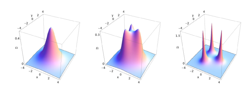
Figure 8: Energy density for a single ${\bf CP}^{2}$ soliton with $m/e^{2}=0$, $1$, $3$.

To illustrate this, in Figure 8, we plot the energy density (or equivalently, the topological charge density) for a BPS soliton (i.e. solving (3.28)), of winding number one, with the target space given by a squashed ${\bf CP}^{2}$. To construct these plots, we first need to choose a vacuum: we have picked $\phi_{i}=0$ which ensures that all partons have equal mass. The first part of the figure shows the lump solution for a round target space, with $m/e^{2}=0$. The soliton is a smooth lump of size $\rho$ with no evidence of partonic structure. Subsequent plots show the soliton solution for the deformed target space. As $m/e^{2}$ increases, the topological charge becomes concentrated around the three points where each $M_{i}$ vanishes, revealing the partonic nature of the object.

In Figure 9, we plot the profile of a single $k=1$ soliton in the deformed target space with $m/e^{2}\approx 3$. The overall scale size, $\rho$, of the soliton is kept fixed, while the orientation modes are changed. The figure shows clearly that these orientation modes govern the relative positions of the partons.

Note that our partons in the ${\bf CP}^{N-1}$ sigma model are not merons for $N\geq 3$. The merons are always associated to topological charge $+1/2$, while our partons carry charge $1/N$.

Collective Coordinates and Parton Positions

While looking at the deformed sigma-model provides the most direct way to see the partonic nature of the soliton, is again possible to see evidence of the partons even when $e^{2}\rightarrow\infty$. First, let us look at the explicit solutions in this limit.

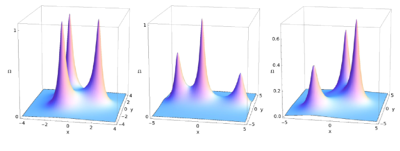
Figure 9: Energy density for a single ${\bf CP}^{2}$ soliton with fixed “scale size” and varying “orientation”.

The soliton with winding $k$ has $2Nk$ collective coordinates. For well separated solitons, these decompose into a position, a scale size and $2N-3$ orientation modes for each lump. However, it is well known that the most general soliton solution is given by specifying $k$ sets of $N$ points, $\{z^{1}_{n}\}\,\ldots\{z^{N}_{n}\}$ with $n=1,\ldots,k$. In the variables $f_{i}$, the soliton solution is given by

$$f_{i}=\prod_{n=1}^{k}(z-z^{i}_{n})$$ (3.29)

This solution includes an implicit choice of vacuum at infinity. Examining (3.27) and (3.22), we see that this choice is the symmetric vacuum $\phi_{i}=0$, in which each parton has mass $M_{i}=m$. In terms of $\hat{\phi}$, this vacuum looks a little less natural: it is $\hat{\phi}_{J}=m(J-N/2)$. This is the same vacuum that we picked when plotting Figures 8 and 9.

It is natural to conjecture that the points $\{z_{n}^{i}\}$ correspond to the positions of the $kN$ underlying partons. To see that this is indeed the case, we translate the soliton solution into toric variables. Tracing through the various definitions, we see that the point in space $f_{i}=0$ corresponds to a point where the mass of the $i^{\rm th}$ hypermultiplet vanishes: $M_{i}=0$. This is identified as the location of the parton.

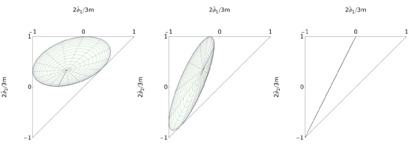
Figure 10: Toric diagrams for ${\bf CP}^{2}$ solitons with different parton positions.

It is useful to illustrate these points with the example of ${\bf CP}^{2}$. The vacuum $\hat{\phi}_{1}=-\hat{\phi}_{2}=-m/2$ sits firmly in the middle of the toric triangle. The images of different lump solutions, corresponding to different ${\bf CP}^{1}$ submanifolds, are shown in figure 10. In each case, the lump image touches each side of the toric diagram at one point: these points are the images of the parton positions. The boundary of the lump image is the image of the unique circle passing through the three parton positions; the interior and exterior of this circle each map bijectively to the interior of the lump image. The centre of the circle and the point at infinity both map to the vacuum. In the case where the three parton positions lie on a straight line, the boundary of the lump image is the image of this line, and includes the vacuum. Then the two half-planes on either side of the line each map to the interior of the lump image. We can also ask what happens as two partons approach each other. In this limit, the ${\bf CP}^{1}$ submanifold touches one corner of the toric diagram, as shown in the third part of the figure.

Parton Quantum Numbers

The parton $Q_{i}$ in the microscopic model carries charges $(+1,-1)$ under $U(1)_{i}\times U(1)_{i+1}$, for each $i=1,\ldots,N$, with $U(1)_{N+1}\equiv U(1)_{1}$. We will now show that it is possible to reconstruct this pattern of electric charges of the partons from the lump solutions.

We again proceed by rewriting the soliton equations in terms of dual variables by using the duality transformation (3.24). In these variables, the soliton equation (3.28) relates each electric field to the variation of the corresponding $\hat{\phi}^{I}$:

$$\hat{F}_{0\alpha}^{I}=\partial_{\alpha}\hat{\phi}_{I}.$$ (3.30)

The electric field $\hat{F}_{0\alpha}^{I}$ is then divergence free except at points where one of the $\hat{\sigma}_{J}$ is ill-defined. From (3.27) and (3.29), we note that these points are at $z=z_{n}^{i}$. Each $\hat{\sigma}_{J}$ has non-trivial winding around two of these points. In particular, $\hat{\sigma}_{J}$ increases by $2\pi$ if we complete an anticlockwise circuit around $z_{n}^{J}$, and $\hat{\sigma}_{J}$ decreases by $2\pi$ if we complete an anticlockwise circuit around $z_{n}^{J+1}$. Following the same arguments as in section 2.3, we deduce that

$$\partial_{\alpha}(\hat{H}_{IJ}\hat{F}_{0\alpha}^{J})=\sum_{n=1}^{k}\left[\delta(z-z_{n}^{I})-\delta(z-z_{n}^{I+1})\right].$$ (3.31)

Just as in the ${\bf CP}^{1}$ case, for given $\{z_{n}^{i}\}$ these equations have a unique solution which specifies a point on the soliton moduli space.

Equation (3.31) shows that each of the $N$ partons sources two neighbouring gauge fields, with the exception of the first and last partons, living at positions $z_{n}^{1}$ and $z_{n}^{N}$. These appear to be charged under just a single gauge field. To reconstruct the full quiver diagram shown in Figure 1, it is simplest to now put back the neutral, decoupled gauge field and work with $F^{i}_{\mu\nu}$ with $i=1,\ldots,N$. The relationship between these $N$ gauge fields and the $(N-1)$ fields $\hat{F}_{\mu\nu}^{I}$ is given in (3.23). In terms of the more symmetric field strengths $F^{i}_{\mu\nu}$, the source equation (3.31) reads

$$\partial_{\alpha}({H}_{ij}{F}_{0\alpha}^{j})=\sum_{n=1}^{k}\left[\delta(z-z_{n}^{i})-\delta(z-z_{n}^{i+1})\right].$$

where $z_{n}^{N+1}\equiv z_{n}^{1}$. This equation is important. It shows that the structure of the soliton captures the quantum numbers of the partons in the UV theory. The soliton is composed of $N$ partons, with the $i^{\rm th}$ parton carrying charge $(+1,-1)$ under $U(1)_{i}\times U(1)_{i+1}$.

The Force Between Solitons

In the case of solitons in the ${\bf CP}^{1}$ sigma model, we saw that the parton quantum numbers could also be determined by the force between a soliton and anti-soliton, which coincides with that between two dipoles. We now ask whether this property extends to the solitons of ${\bf CP}^{N-1}$. Can we interpret the soliton anti-soliton force as the sum of dipoles with charges dictated by the quiver? The answer appears to be no.

The computation of the force between a soliton and anti-soliton in the ${\bf CP}^{N-1}$ sigma model was performed many years ago in [29]. We’ll denote the collective coordinates of the instanton by $\{z^{i}\}$ as in (3.29), while those of the anti-instanton are $\{y^{i}\}$. If the two objects are separated by distance $r$, the interaction potential is given by

$$V_{\rm int}=-\frac{4m}{r^{2}}\left[\sum_{i=1}^{N}z_{i}y_{i}-\frac{1}{N}\left(\sum_{i=1}^{N}z_{i}\right)\left(\sum_{j=1}^{N}y_{i}\right)\right]+{\rm h.c.}$$

This does not capture the key features of the quiver diagram. In particular, this force treats all partons on the same footing. The $i^{\rm th}$ parton, at position $z^{i}$, interacts with all the anti-partons rather than just the $i^{\rm th}$ and $(i+1)^{\rm th}$ as naively suggested by the classical quiver diagram. It appears that the filter of renormalization group flow is simply too strong and this low-energy force computation too myopic to determine the partonic quantum numbers. Thankfully the dual Bogomolnyi equation described above does the job for us.

4 What Does This Tell Us About Yang-Mills Instantons?

In $d=4+1$ spacetime dimensions, Yang-Mills theories are non-renormalizable. Arguments involving supersymmetry and string theory show that these theories have a well-defined ultra-violet completion when equipped with 8 or 16 supercharges [30]. Yet little is known about the properties of the UV degrees of freedom.

The story is especially interesting for the theory with 16 supercharges which has a UV fixed point governed by the $(2,0)$ superconformal theory in $d=5+1$ dimensions. The $(2,0)$ theory arises as the low-energy limit of $N$ M5-branes and, famously, has a number of degrees of freedom that scales as $N^{3}$ [31]. Understanding the kind of mathematical structure that gives rise to this $N^{3}$ scaling remains an important challenge.

When compactified on a circle of radius $R$, only $\sim N^{2}$ degrees of freedom remain massless and, at long distances, the $(2,0)$ theory reduces to $5d$, maximally supersymmetric $U(N)$ Yang-Mills with gauge coupling $g^{2}=8\pi^{2}R$. Instantons in this theory, obeying $F={}^{\star}F$, are BPS particles and are identified with the Kaluza-Klein (KK) modes coming from six dimensions [32],

$$M_{\rm inst}=\frac{8\pi^{2}}{g^{2}}=\frac{1}{R}=M_{KK}$$

These instantons come with a puzzle. Upon quantization, the scaling mode $\rho\in{\bf R}^{+}$ of the instanton gives rise to a continuous spectrum above $M_{\rm inst}$. This is odd behaviour for a one-particle state in a quantum field theory. We propose that this continuous spectrum arises because the instanton should be interpreted as an $N$ particle state. Moreover, motivated by the similarity with the sigma-model described in the previous sections, we conjecture that the $N$ partons inside the instanton are related to the UV degrees of freedom which complete the Yang-Mills theory at high energies.

Let us start by providing circumstantial evidence for this proposal. First we can ask where the crossover from $\sim N^{2}$ to $\sim N^{3}$ degrees of freedom occurs. This was studied in [33] using supergravity techniques where it was shown that the transition happens at temperature

$$T\sim\frac{8\pi^{2}}{g^{2}N}$$

Indeed, this had to be the case: the theory is strongly coupled at energies $E\sim 1/g^{2}N$ and this is where the new degrees of freedom must kick in. This mass scale points firmly at the existence of instantonic partons.

The existence of modes carrying fractional KK momentum is familiar in compactified Yang-Mills theories, where they arise in the presence of a Wilson line. Such modes occur whenever $N$ branes wrapped on the circle combine to form a single “long” brane wrapped $N$ times. Behaviour of this type was important in the original work on black hole entropy counting [34, 35].

It is also worth mentioning some further numerological evidence for the partonic interpretation of instantons. The $N^{3}$ scaling for M5-branes can be refined by an anomaly computation [36] whose coefficient provides the subleading term in the number of degrees of freedom on $N$ M5-branes: $c(su(N))=N^{3}-N$. A generalization of this formula to other $G=\,$ADE theories was conjectured by Intriligator to be [37],

$$c(G)=C_{2}(G)\,|G|$$

where $C_{2}(G)$ is the dual Coxeter number (normalized such that $C_{2}(su(N))=N)$ and $|G|$ is the dimension of the group. This fits nicely with our partonic interpretation of instantons since the dimension of the moduli space of a single instanton is $4C_{2}(G)$, implying the existence of $C_{2}(G)$ partons in general. The presence of $|G|$ in the anomaly coefficient is perhaps hinting that each of these partons transforms in the adjoint of the gauge group $G$.

In the case of sigma-model solitons, we have seen above that a detailed study allows us to reconstruct properties of the high-energy theory. Can we do something similar for Yang-Mills instantons? We hope to return to this question in future work. Here we limit ourselves to a few simple observations and speculations. Firstly, the instanton solution has only magnetic components of the five-dimensional gauge field turned on. Yet, in five dimensions, magnetic charge is naturally carried by string-like objects. So perhaps each parton is itself a loop of string. Indeed, the caloron picture [25, 26] reveals $N$ strings inside the instanton but, as we described in Section 2, in the case of sigma-model lumps calorons were not directly related to partons. Strings were also found lurking inside instantons in [38, 39] in the context of dyonic instantons [40].

In the context of the sigma-model, the force between a lump and anti-lump spectacularly revealed the partonic quantum numbers for ${\bf CP}^{1}$, but proved more myopic in the case of ${\bf CP}^{N-1}$. For Yang-Mills instantons, the force was computed in [41]. An instanton of size $\rho$ and an anti-instanton of size $\bar{\rho}$, separated by a distance $r\gg\rho,\bar{\rho}$ feel the attractive potential

$$V=-\frac{32\pi^{2}}{g^{2}}\frac{\rho^{2}\bar{\rho}^{2}}{r^{4}}\,C_{ab}\,\bar{\eta}^{a}_{\mu\nu}\eta^{b}_{\mu\lambda}\hat{r}_{\nu}\hat{r}_{\lambda}$$

The fact that the force is quadratic in $\rho$, rather than linear, is again indicative of loop-like objects as befits a magnetic dipole. Here $C_{ab}$ describes the relative orientation of the two instantons within the gauge group. Aligned instantons, with $C_{ab}=\delta_{ab}$ feel the maximum force. However, in contrast to the situation with sigma-model lumps, instantons can hide from each. If they sit in commuting $SU(2)$ factors in the gauge group, the instanton and anti-instanton feel no force. (A similar phenomenon is not allowed in the case of the sigma-model because both lump and anti-lump solutions are required to asymptote to the same vacuum). Needless to say, it would be very interesting to interpret the instanton force formula in terms of partons.

Finally, perhaps the most important question is to determine the confinement mechanism that binds the partons inside the instanton yet allows them to move freely. In the case of the sigma-model lump this arose due to the log-divergent energy arising from the long-range fields of the parton. However, as discussed above, this divergence reveals itself in the moduli space metric for lumps. There is no hint of such a divergence in the moduli space metric for instantons, suggesting that the confinement mechanism is something different in this case. In particular, this means that the merons discussed in [41] are not the partons of interest: as well as having topological charge $1/2$ instead of $1/N$, they have $F_{\mu\nu}\sim 1/r^{2}$ giving rise to a log-divergent energy. It appears that the confinement mechanism at play inside Yang-Mills instantons is somewhat more subtle. Perhaps the deconstruction of the $(2,0)$ theories presented in [42, 43] can shed light on this issue.

References

- [1]
- [2] A. A. Belavin, V. A. Fateev, A. S. Schwarz and Yu. S. Tyupkin, “Quantum Fluctuations Of Multi-Instanton Solutions,” Phys. Lett. B 83, 317 (1979).
- [3] D. Diakonov and M. Maul, “On statistical mechanics of instantons in the model,” Nucl. Phys. B 571, 91 (2000) [arXiv:hep-th/9909078].
- [4] D. T. Son, M. A. Stephanov and A. R. Zhitnitsky, “Instanton interactions in dense-matter QCD,” Phys. Lett. B 510, 167 (2001) [arXiv:hep-ph/0103099].
- [5] A. R. Zhitnitsky, “Confinement-deconfinement phase transition and fractional instanton quarks in dense matter,” arXiv:hep-ph/0601057.
- [6] A. Parnachev and A. R. Zhitnitsky, “Phase Transitions, theta Behavior and Instantons in QCD and its Holographic Model,” Phys. Rev. D 78, 125002 (2008) [arXiv:0806.1736].
- [7] A. S. Gorsky, V. I. Zakharov and A. R. Zhitnitsky, “On Classification of QCD defects via holography,” arXiv:0902.1842 [hep-ph].
- [8] K. A. Intriligator and N. Seiberg, “Mirror symmetry in three dimensional gauge theories,” Phys. Lett. B 387, 513 (1996) [arXiv:hep-th/9607207].
- [9] N. Dorey, V. V. Khoze, M. P. Mattis, D. Tong and S. Vandoren, “Instantons, three-dimensional gauge theory, and the Atiyah-Hitchin manifold,” Nucl. Phys. B 502, 59 (1997) [arXiv:hep-th/9703228].
- [10] T. Eguchi and A. J. Hanson, “A͡symptotically Flat Selfdual Solutions To Euclidean Gravity,” Phys. Lett. B 74, 249 (1978).
- [11] O. Aharony, A. Hanany, K. A. Intriligator, N. Seiberg and M. J. Strassler, “Aspects of N = 2 supersymmetric gauge theories in three dimensions,” Nucl. Phys. B 499, 67 (1997) [arXiv:hep-th/9703110].
- [12] M. Aganagic, K. Hori, A. Karch and D. Tong, “Mirror symmetry in 2+1 and 1+1 dimensions,” JHEP 0107, 022 (2001) [arXiv:hep-th/0105075].
- [13] V. Borokhov, A. Kapustin and X. k. Wu, “Monopole operators and mirror symmetry in three dimensions,” JHEP 0212, 044 (2002) [arXiv:hep-th/0207074].
- [14] D. J. Gross, “Meron Configurations In The Two-Dimensional Sigma Model,” Nucl. Phys. B 132, 439 (1978).
- [15] M. Eto, T. Fujimori, S.B. Gudnason, K. Konishi, K. Ohashi, T. Nagashima, M. Nitta, W. Vinci, “Fractional Vortices and Lumps”, arXiv:0905.3540 [hep-th].
- [16] M. Eto, T. Fujimori, S. B. Gudnason, M. Nitta and K. Ohashi, “SO and USp Kähler and Hyper-Kähler Quotients and Lumps,” Nucl. Phys. B 815, 495 (2009) [arXiv:0809.2014 [hep-th]].
- [17] R. S. Ward, “Slowly Moving Lumps In The Model In (2+1)-Dimensions,” Phys. Lett. B 158, 424 (1985).
- [18] V. A. Fateev, I. V. Frolov and A. S. Shvarts, “Quantum Fluctuations Of Instantons In The Nonlinear Sigma Model,” Nucl. Phys. B 154, 1 (1979).
- [19] B. Berg and M. Luscher, “Computation Of Quantum Fluctuations Around Multi-Instanton Fields From Exact Green’s Functions: The Case,” Commun. Math. Phys. 69, 57 (1979).
- [20] D. Tong, “The moduli space of BPS domain walls,” Phys. Rev. D 66, 025013 (2002) [arXiv:hep-th/0202012].
- [21] M. Eto, T. Fujimori, Y. Isozumi, M. Nitta, K. Ohashi, K. Ohta and N. Sakai, “Non-Abelian vortices on cylinder: Duality between vortices and walls,” Phys. Rev. D 73, 085008 (2006) [arXiv:hep-th/0601181].
- [22] F. Bruckmann, “Instanton constituents in the O(3) model at finite temperature,” Phys. Rev. Lett. 100, 051602 (2008) [arXiv:0707.0775 [hep-th]].
- [23] D. Harland, “Kinks, chains, and loop groups in the sigma models,” arXiv:0902.2303 [hep-th].
- [24] W. Brendel, F. Bruckmann, L. Janssen, A. Wipf and C. Wozar, “Instanton constituents and fermionic zero modes in twisted models,” arXiv:0902.2328 [hep-th].
- [25] K. M. Lee and P. Yi, “Monopoles and instantons on partially compactified D-branes,” Phys. Rev. D 56, 3711 (1997) [arXiv:hep-th/9702107].
- [26] T. C. Kraan and P. van Baal, “Periodic instantons with non-trivial holonomy,” Nucl. Phys. B 533, 627 (1998) [arXiv:hep-th/9805168].
- [27] S. R. Coleman, “More About The Massive Schwinger Model,” Annals Phys. 101, 239 (1976).
- [28] K. M. Lee, E. J. Weinberg and P. Yi, “The Moduli Space of Many BPS Monopoles for Arbitrary Gauge Groups,” Phys. Rev. D 54, 1633 (1996) [arXiv:hep-th/9602167].
- [29] K. Bardakci, D. G. Caldi and H. Neuberger, “Dominant Euclidean Configurations For All N,” Nucl. Phys. B 177, 333 (1981).
- [30] N. Seiberg, “Five dimensional SUSY field theories, non-trivial fixed points and string dynamics,” Phys. Lett. B 388, 753 (1996) [arXiv:hep-th/9608111].
- [31] I. R. Klebanov and A. A. Tseytlin, “Entropy of Near-Extremal Black p-branes,” Nucl. Phys. B 475, 164 (1996) [arXiv:hep-th/9604089].
- [32] M. Rozali, “Matrix theory and U-duality in seven dimensions,” Phys. Lett. B 400, 260 (1997) [arXiv:hep-th/9702136].
- [33] N. Itzhaki, J. M. Maldacena, J. Sonnenschein and S. Yankielowicz, “Supergravity and the large N limit of theories with sixteen supercharges,” Phys. Rev. D 58, 046004 (1998) [arXiv:hep-th/9802042].
- [34] S. R. Das and S. D. Mathur, “Excitations of D-strings, Entropy and Duality,” Phys. Lett. B 375, 103 (1996) [arXiv:hep-th/9601152].
- [35] J. M. Maldacena and L. Susskind, “D-branes and Fat Black Holes,” Nucl. Phys. B 475, 679 (1996) [arXiv:hep-th/9604042].
- [36] J. A. Harvey, R. Minasian and G. W. Moore, “Non-abelian tensor-multiplet anomalies,” JHEP 9809, 004 (1998) [arXiv:hep-th/9808060].
- [37] K. A. Intriligator, “Anomaly matching and a Hopf-Wess-Zumino term in 6d, N = (2,0) field theories,” Nucl. Phys. B 581, 257 (2000) [arXiv:hep-th/0001205].
- [38] S. Kim and K. M. Lee, “Dyonic instanton as supertube between D4 branes,” JHEP 0309, 035 (2003) [arXiv:hep-th/0307048].
- [39] M. Y. Choi, K. K. Kim, C. Lee and K. M. Lee, “Higgs Structures of Dyonic Instantons,” JHEP 0804, 097 (2008) [arXiv:0712.0735 [hep-th]].
- [40] N. D. Lambert and D. Tong, “Dyonic instantons in five-dimensional gauge theories,” Phys. Lett. B 462, 89 (1999) [arXiv:hep-th/9907014].
- [41] C. G. Callan, R. F. Dashen and D. J. Gross, “Toward a theory of the strong interactions,” Phys. Rev. D 17, 2717 (1978).
- [42] N. Arkani-Hamed, A. G. Cohen, D. B. Kaplan, A. Karch and L. Motl, “Deconstructing (2,0) and little string theories,” JHEP 0301, 083 (2003) [arXiv:hep-th/0110146].
- [43] D. Gaiotto, “N=2 dualities,” arXiv:0904.2715 [hep-th]; D. Gaiotto and J. Maldacena, “The gravity duals of N=2 superconformal field theories,” arXiv:0904.4466 [hep-th].
- [44] P. C. Nelson and S. R. Coleman, “What Becomes Of Global Color,” Nucl. Phys. B 237, 1 (1984).