Abstract

Supersymmetric contributions to time independent asymmetry in $B^{0}_{s}\to J/\psi\phi$ process are analyzed in the view of the recent Tevatron experimental measurements. We show that the experimental limits of the mass difference $\Delta M_{B_{s}}$ and the mercury EDM significantly constrain the SUSY contribution to $B^{0}_{s}-\bar{B}^{0}_{s}$ mixing, so that $\sin 2\beta_{s}\raise 1.29167pt\hbox{$\;<$\kern-7.5pt\raise-4.73611pt\hbox{$\sim\;$}}0.1$. We also point out that the one loop SUSY contribution to $B^{0}_{s}\to J/\psi\phi$ decay can be important and can lead to large indirect CP asymmetries which are different for different polarization states. These new physics effects in the decay amplitude can be consistent with CP measurements in the $B_{d}$ system.

Supersymmetry and CP violation in $B^{0}_{s}-\bar{B}^{0}_{s}$ mixing and $B^{0}_{s}\to J/\psi\phi$ decay

1 Introduction

Recently, CDF and $D0$ collaborations have announced the observation of CP violation in $B_{s}^{0}-\bar{B}_{s}^{0}$ mixing. The following results, for $B^{0}_{s}$-mixing CP violating phase, have been reported [1, 2]:

$$2\beta_{s} = 0.57~{}^{+0.30}_{-0.24}~{}({\rm stat.})~{}^{+0.02}_{-0.07}~{}({\rm syst.})~{}~{}~{}~{}~{}~{}~{}~{}~{}~{}~{}~{}~{}~{}~{}~{}~{}~{}~{}~{}~{}~{}(DO),$$ (1)

$$2\beta_{s} \in \left[0.32,2.82\right](68\%)~{}~{}~{}~{}~{}~{}~{}~{}~{}~{}~{}~{}~{}~{}~{}~{}~{}~{}~{}~{}~{}~{}~{}~{}~{}~{}~{}~{}~{}~{}~{}~{}~{}~{}~{}~{}(CDF).$$ (2)

These results indicate that the phase $\beta_{s}$ deviates more that $3\sigma$ from the Standard Model (SM) prediction [3]. Therefore, the experimental observation of CP violation in $B^{0}_{s}$ mixing, along with the Belle and Baber measurement for direct and indirect CP asymmetries of $B_{d}$ decays, open the possibility of probing new physics effect at low energy.

It is a common feature for any physics beyond the SM to possess additional sources of CP violation besides the SM phase in quark mixing matrix. In supersymmetric extension of the SM, the soft SUSY breaking terms are in general complex and can give new contributions to CP violating processes. The SUSY CP violating phases can be classified as flavor independent phases, like the phases of the gaugino masses and $\mu$ term, and flavor-dependent phases, like the phases of the off-diagonal $A$-terms. The flavor independent phases are stringently constrained by the experimental limits on electric dipole moment (EDM) of electron and neutron. However, the flavor dependent phases are much less constrained. This may imply that SUSY CP violation has a flavor off diagonal character just as in the Standard Model. In this case the origin of CP violation is closely related to the origin of the flavor structures rather than the origin of SUSY breaking [4].

The SUSY flavor dependent phases can induce sizeable contributions to direct and indirect CP asymmetries of $B_{d}$ decays [5, 6, 7], as in $B_{d}\to\phi K_{S}$, $B_{d}\to\eta^{\prime}K_{S}$ and $B_{d}\to K\pi$ which show some discrepancy with the SM expectation. In this paper we revisit the supersymmetric contributions to $B_{s}^{0}-\bar{B}_{s}^{0}$ mixing. We investigate the possibility that SUSY may be responsible for the large observed value of $B_{s}$ mixing phase without enhancing the mass difference $\Delta M_{s}$ over the measured value. In addition, we analyze the one loop SUSY contribution to $B^{0}_{s}\to J/\psi\phi$ decay, which turns out to be important and can lead to a large indirect CP asymmetry.

The paper is organized as follows. In section 2 we analyze the possible new physics contributions to $B_{s}^{0}-\bar{B}_{s}^{0}$ mixing and indirect CP asymmetry of $B_{s}^{0}\to J/\psi\phi$, taking into account the constraints imposed by the experimental measurments of the mass difference $\Delta M_{B_{s}}$ and the mercury EDM. In section 3 we discuss the supersymmetric contributions to effective Hamiltonian for $\Delta B=2$ and $\Delta B=1$ transitions. In section 4 we show that the mercury EDM impose stringent constraints on the supersymmetric contribution to the phase $\beta_{s}$, such that the $B_{s}^{0}$ mixing phase can not exceed 0.1. In section 5 we analyze the supersymmetric contribution to the $B_{s}^{0}\to J/\psi\phi$ decay. We emphasize that the one loop SUSY contribution to $B_{s}^{0}\to J/\psi\phi$ can be important and lead to large indirect CP asymmetries which are in general different for different polarization states. Finally, we give our conclusions in section 6.

2 $B_{s}^{0}-\bar{B}_{s}^{0}$ mixing and CP asymmetry in $B_{s}^{0}\to J/\psi\phi$

In the the $B_{s}^{0}$ and $\bar{B}_{s}^{0}$ system, the flavor eigenstates are given by $B^{0}_{s}=(\bar{b}s)$ and $\bar{B}_{s}^{0}=(b\bar{s})$. The corresponding mass eigenstates are defined as $B_{L}=pB_{s}^{0}-q\bar{B}_{s}^{0}$ and $B_{H}=pB_{s}^{0}+q\bar{B}_{s}^{0}$, where $L$ and $H$ refer to light and heavy mass eigenstates respectively. The mixing angles $q$ and $p$ are defined in terms of the transition matrix element ${\cal M}_{12}=\langle B_{s}^{0}|H_{eff}^{\Delta B=2}|\bar{B}_{s}^{0}\rangle$, where $H_{eff}^{\Delta B=2}$ is the effective Hamiltonian responsible for $\Delta B=2$ transitions:

$$\frac{q}{p}=\sqrt{\frac{{\cal M}_{12}^{*}}{{\cal M}_{12}}},$$ (3)

where we assumed that $\Delta\Gamma_{B_{s}}\ll\Delta M_{B_{s}}$ and $\Delta\Gamma_{B_{s}}\ll\Gamma_{B_{s}}^{total}$. The strength of $B_{s}^{0}-\bar{B}_{s}^{0}$ mixing is described by the mass deference

$$\Delta M_{B_{s}}=M_{B_{H}}-M_{B_{L}}=2{\rm Re}\left[\frac{q}{p}{\cal M}_{12}\right]=2|{\cal M}_{12}(B_{s})|.$$ (4)

The decay $B^{0}_{s}\to J/\psi\phi$ involves vector-vector final states with three polarization amplitudes. Therefore, an angular distribution is necessary to separate out the three polarizations for a measurement of indirect CP violation without dilution. The amplitudes for the decay of $B_{s}^{0}\to f$ and $\bar{B}_{s}^{0}\to f$ are given by $A^{\lambda}(f)=\langle f|H_{eff}^{\Delta B=1}|B_{s}^{0}\rangle$ and $\bar{A}^{\lambda}(f)=\langle f|H_{eff}^{\Delta B=1}|\bar{B}_{s}^{0}\rangle$ with

$$\bar{\rho}^{\lambda}(f)=\frac{\bar{A}^{\lambda}(f)}{A^{\lambda}(f)}=\frac{1}{\rho^{\lambda}(f)}.$$ (5)

Here, $\lambda$, is the polarization index. Therefore, the source of CP violation in decays to CP eigenstates with oscillation are: oscillation if $q/p\neq 1$, decay if $\bar{\rho}^{\lambda}(f)\neq 1$, both oscillation and decay if $\{q/p,\bar{\rho}^{\lambda}(f)\}\neq 1$. The time dependent CP asymmetry of $B_{s}^{0}\to J/\psi\phi$, for each polarization state $\lambda$, is given by

$$A^{\lambda}_{J/\psi\phi}(t) = \frac{\Gamma^{\lambda}(\bar{B}_{s}^{0}(t)\to J/\psi\phi)-\Gamma^{\lambda}(B_{s}^{0}(t)\to J/\psi\phi)}{\Gamma^{\lambda}(\bar{B}_{s}^{0}(t)\to J/\psi\phi)+\Gamma^{\lambda}(B_{s}^{0}(t)\to J/\psi\phi)},$$ (6)

$$= C^{\lambda}_{J/\psi\phi}\cos\Delta M_{B_{s}}t+S^{\lambda}_{J/\psi\phi}\sin\Delta M_{B_{s}}t,$$

where $C^{\lambda}_{J/\psi\phi}$ and $S^{\lambda}_{J/\psi\phi}$ represent the direct and the mixing CP asymmetry, respectively and they are given by

$$C^{\lambda}_{J/\psi\phi}=\frac{|\bar{\rho}^{\lambda}(J/\psi\phi)|^{2}-1}{|\bar{\rho}^{\lambda}(J/\psi\phi)|^{2}+1},~{}~{}~{}~{}~{}~{}~{}~{}~{}~{}~{}S^{\lambda}_{J/\psi\phi}=\eta^{\lambda}\frac{2{\rm Im}\left[\frac{q}{p}\bar{\rho}^{\lambda}(J/\psi\phi)\right]}{|\bar{\rho}^{\lambda}(J/\psi\phi)|^{2}+1},$$ (7)

where $\eta^{\lambda}$ is $\pm$ depending on the polarization states. In the SM, the mixing CP asymmetry in $B^{0}_{s}\to J/\psi\phi$ process is the same for all polarization, to a very good approximation, up to a sign. Hence we will omit the polarization index when discussing the SM results. We have in the SM,

$$\sin 2\beta_{s}=S_{J/\psi\phi}.$$ (8)

If $\rho(J/\psi\phi)=1$, which is the case in SM, then $\beta_{s}$ is defined as $2\beta_{s}=\arg\left[{\cal M}_{12}(B_{s})\right]$.

In the SM, the mass difference is given by

$$\Delta M_{B_{s}}^{SM}=\frac{G_{F}^{2}}{6\pi^{2}}\eta_{B}m_{B}(\hat{B}_{B_{s}}F_{B_{s}}^{2})M_{W}^{2}|V_{ts}|^{2}S_{0}(x_{t}).$$ (9)

One may estimate the SM contribution to $\Delta M_{B_{s}}$ through the ratio $\Delta M_{B_{s}}^{SM}/\Delta M_{B_{d}}^{SM}$, where the uncertainties due to short-distance effect cancel:

$$\frac{\Delta M_{B_{s}}^{SM}}{\Delta M_{B_{d}}^{SM}}=\frac{M_{B_{s}}}{M_{B_{d}}}\frac{B_{B_{s}}f_{B_{s}}^{2}}{B_{B_{s}}f_{B_{s}}^{2}}\frac{|V_{ts}|^{2}}{|V_{td}|^{2}}.$$ (10)

We can assume that $\Delta M_{B_{d}}^{SM}=\Delta M_{B_{d}}^{exp}\simeq 0.507{\rm ps}^{-1}$. Thus, for quark mixing angle $\gamma\simeq 67^{~{}\circ}$, one finds $\Delta M_{B_{s}}^{SM}\simeq 15{\rm ps}^{-1}$, which is consistent with the recent results reported by CDF and $D0$:

$$\Delta M_{B_{s}} = 17.77\pm 0.10({\rm stat.})\pm 0.07({\rm syst.})~{}~{}~{}~{}~{}~{}~{}~{}~{}~{}~{}~{}~{}~{}~{}~{}~{}~{}(CDF),$$ (11)

$$\Delta M_{B_{s}} = 18.53\pm 0.93({\rm stat.})\pm 0.30({\rm syst.})~{}~{}~{}~{}~{}~{}~{}~{}~{}~{}~{}~{}~{}~{}~{}~{}~{}~{}(CDF).$$ (12)

On the other hand, the SM contribution ($\rho(J/\psi\phi)=1$) to the CP asymmetry $S_{J/\psi\phi}$ is given by

$$S_{J/\psi\phi}=\sin 2\beta_{s}^{SM},~{}~{}~{}~{}{\rm with}~{}~{}~{}~{}\beta_{s}^{SM}=\arg\left(\frac{-V_{cs}V_{cb}^{*}}{V_{ts}V_{tb}^{*}}\right)\simeq{\cal O}(0.01),$$ (13)

where $V_{ij}$ are the elements of the CKM quark mixing matrix. This result clearly conflicts with the experimental measurements reported in Eqs.(1,2). Therefore, a confirmation for these measurements would be no doubt signal for new physics beyond the SM. As indicated above, $S_{J/\psi\phi}$ carries a polarization index corresponding to the three final state polarization, however in the SM the mixing induced asymmetries are the same( up to a sign) for the three polarizations.

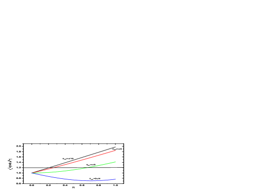
Figure 1: The constraint on $R=|A_{NP}/A_{SM}|$ in case of $\theta=\pi/10,\pi/4,\pi/2$ and $3\pi/4$.

In a model independent way, the effect of new physics (NP), with $\rho(J/\psi\phi)=1$, can be described by the dimensionless parameter $r_{s}^{2}$ and a phase $2\theta_{s}$ defined as follows:

$$r_{s}^{2}e^{2i\theta_{s}}=\frac{{\cal M}_{12}(B_{s})}{{\cal M}^{SM}_{12}(B_{s})}=1+\frac{{\cal M}^{NP}_{12}(B_{s})}{{\cal M}^{SM}_{12}(B_{s})},$$ (14)

Therefore, $\Delta M_{B_{s}}=2|{\cal M}^{SM}_{12}(B_{s})|r_{s}^{2}=\Delta M^{SM}_{B_{s}}r_{s}^{2}$. In this respect, $r_{s}^{2}$ is bounded by $r_{s}^{2}\raise 1.29167pt\hbox{$\;<$\kern-7.5pt\raise-4.73611pt\hbox{$\sim\;$}}\Delta M^{exp}_{B_{s}}/\Delta M^{SM}_{B_{s}}\raise 1.29167pt\hbox{$\;<$\kern-7.5pt\raise-4.73611pt\hbox{$\sim\;$}}1.2$. This constrains the ratio between the NP and SM amplitudes defined as, $R=|A_{NP}/A_{SM}|$, as follow:

$$\left|1+Re^{i\theta_{NP}}\right|\raise 1.29167pt\hbox{$\;<$\kern-7.5pt\raise-4.73611pt\hbox{$\sim\;$}}1.2$$ (15)

Note that for vanishing NP phase, i.e.$\theta_{NP}=0$, one find that $R\raise 1.29167pt\hbox{$\;<$\kern-7.5pt\raise-4.73611pt\hbox{$\sim\;$}}0.2$. However, for $\theta_{NP}\neq 0$, the constrain on $R$ is relaxed as shown in Fig. 1. It is clear that $R$ can be of order one if the NP phase is tuned to be within the range: $\pi/2<\theta_{NP}<\pi$, .

In the presence of NP contribution, the CP asymmetry $B^{0}_{s}\to J/\psi\phi$ is modified and now we have

$$S_{J/\psi\phi}=\sin 2\beta_{eff}=\sin(2\beta_{s}^{SM}+2\theta_{s}),$$ (16)

where

$$2\theta_{s}=\arg\left(1+Re^{\theta_{NP}}\right).$$ (17)

Therefore, in order to enhance the NP effects, large values of $R$ are required. Now we consider the effect of NP that leads to ${\rm Im}[\rho(J/\psi\phi)]\neq 1$. Let us write the amplitude as

$$\bar{A}^{\lambda}(J/\psi\phi)=\bar{A}^{\lambda}_{SM}(J/\psi\phi)+\bar{A}^{\lambda}_{NP}(J/\psi\phi),$$ (18)

and define,

$$\frac{A^{\lambda}(J/\psi\phi)}{A^{\lambda}_{SM}(J/\psi\phi)}=S_{A}^{\lambda}e^{i\theta^{\lambda}_{A}},$$ (19)

where $\theta^{\lambda}_{A}$ is a weak phase, $\lambda$ is the polarization index, and we have assumed that the strong phases in the amplitude ratio cancel. One can now write $\bar{\rho}(J/\psi\phi)$ as

$$\bar{\rho}(J/\psi\phi)=e^{-2i\theta^{\lambda}_{A}}.$$ (20)

Thus, one obtains,

$$\frac{q}{p}\bar{\rho}(J/\psi\phi)=e^{-2i(\beta_{SM}+\theta_{s}+\theta^{\lambda}_{A})}.$$ (21)

In this case, the CP asymmetry $B^{0}_{s}\to J/\psi\phi$ is modified and now we have,

$$S_{J/\psi\phi}=\sin(2\beta_{s}^{SM}+2\theta_{s}+2\theta^{\lambda}_{A}).$$ (22)

However, as pointed out in Ref.[5], this parametrization is true only when the strong phase of the full amplitude is assumed to be the same as the SM amplitude. In fact, as discussed in Ref. [8], the NP strong phase can be different and is generally smaller than the SM strong phase thus invalidating the assumption about strong phases made in Eq.(19). In general, the SM and NP amplitude can be parameterized as:

$$A^{\lambda}_{{\rm SM}}=|A^{\lambda}_{{\rm SM}}|e^{i\delta^{\lambda}_{{\rm SM}}},~{}~{}~{}~{}~{}A^{\lambda}_{{\rm NP}}=\sum_{i}|A^{\lambda}_{{i\rm NP}}|e^{i\theta^{\lambda}_{{i\rm NP}}}e^{i\delta^{\lambda}_{{i\rm NP}}},$$ (23)

where $\delta^{\lambda}_{i\rm NP}$ are the strong phases and $\theta^{\lambda}_{{i\rm NP}}$ are the CP violating phase. If there is one dominant NP amplitude then we can parametrize the NP amplitude as

$$A^{\lambda}_{{\rm NP}} = |A^{\lambda}_{{\rm NP}}|e^{i\theta^{\lambda}_{{i\rm NP}}}e^{i\delta^{\lambda}_{{i\rm NP}}}\ .$$ (24)

Thus, the CP asymmetry $S_{J/\psi\phi}$ can be approximately written as:

$$S_{J/\psi\phi}^{\lambda}=\sin(2\beta_{s}^{SM}+2\theta_{s})+2r_{A}^{\lambda}\cos(2\beta_{s}^{SM}+2\theta_{s})\sin\theta^{\lambda}_{{\rm NP}}\cos\delta^{\lambda},$$ (25)

where $r_{A}^{\lambda}=|A_{{\rm NP}}^{\lambda}/A_{{\rm SM}}^{\lambda}|$ and $\delta^{\lambda}=\delta^{\lambda}_{{\rm SM}}-\delta^{\lambda}_{{\rm NP}}$. Here $\lambda$ represents the various polarization states of the vector-vector final state.

In the SUSY case, considered in this paper, there will be two dominant operators. In this case we can write the new physics amplitude as,

$$A^{\lambda}_{{\rm NP}}=|A^{\lambda}_{{1\rm NP}}|e^{i\theta^{\lambda}_{{1\rm NP}}}e^{i\delta^{\lambda}_{{1\rm NP}}}+|A^{\lambda}_{{2\rm NP}}|e^{i\theta^{\lambda}_{{2\rm NP}}}e^{i\delta^{\lambda}_{{2\rm NP}}}\ .$$ (26)

Now using the result in Ref. [8], we will neglect the NP strong phase and hence the new physics amplitude can be rewritten as an effective single NP amplitude,

$$A^{\lambda}_{{\rm NP}} = |A^{\lambda}_{{\rm NP}}|e^{i\theta^{\lambda}_{{\rm NP}}}$$

$$\tan{\theta^{\lambda}_{{\rm NP}}} = \frac{|A^{\lambda}_{{1\rm NP}}|\sin{\theta^{\lambda}_{1\rm NP}}+|A^{\lambda}_{{2\rm NP}}|\sin{\theta^{\lambda}_{2\rm NP}}}{|A^{\lambda}_{{1\rm NP}}|\cos{\theta^{\lambda}_{1\rm NP}}+|A^{\lambda}_{{2\rm NP}}|\cos{\theta^{\lambda}_{2\rm NP}}}$$

$$|A^{\lambda}_{{\rm NP}}| = \sqrt{\left(|A^{\lambda}_{{1\rm NP}}|\sin{\theta^{\lambda}_{1\rm NP}}+|A^{\lambda}_{{2\rm NP}}|\sin{\theta^{\lambda}_{2\rm NP}}\right)^{2}+\left(|A^{\lambda}_{{1\rm NP}}|\cos{\theta^{\lambda}_{1\rm NP}}+|A^{\lambda}_{{2\rm NP}}|\cos{\theta^{\lambda}_{2\rm NP}}\right)^{2}}~{}~{}~{}~{}~{}~{}$$ (27)

Hence the expression in Eq.(25) can still be used provided we set the NP strong phases to zero.

3 Supersymmetric contributions to $\Delta B=2$ and $\Delta B=1$ transitions

In this section, we analyze the SUSY contribution to the $B_{s}^{0}-\bar{B}_{s}^{0}$ mixing and $B_{s}^{0}\to J/\psi\phi$ decay. As pointed out in Ref.[9], gluino exchanges through $\Delta B=2$ box diagrams give the dominant contribution to $B_{s}^{0}-\bar{B}_{s}^{0}$ mixing, while the chargino exchanges are subdominant and can be neglected. The general $H_{\mathrm{eff}}^{\Delta B=2}$ induced by gluino exchanges can be expressed as

$$H_{\mathrm{eff}}^{\Delta B=2}=\sum_{i=1}^{5}C_{i}(\mu)Q_{i}(\mu)+\sum_{i=1}^{3}\tilde{C}_{i}(\mu)\tilde{Q}_{i}(\mu)+h.c.,$$ (28)

where $C_{i}(\mu)$, $\tilde{C}_{i}(\mu)$, $Q_{i}(\mu)$ and $\tilde{Q}_{i}(\mu)$ are the Wilson coefficients and operators respectively normalized at the scale $\mu$, with,

$$Q_{1} = \bar{s}^{\alpha}_{L}\gamma_{\mu}b_{L}^{\alpha}~{}\bar{s}^{\beta}_{L}\gamma_{\mu}b_{L}^{\beta},$$ (29)

$$Q_{2} = \bar{s}^{\alpha}_{R}b_{L}^{\alpha}~{}\bar{s}^{\beta}_{R}b_{L}^{\beta},$$ (30)

$$Q_{3} = \bar{s}^{\alpha}_{R}b_{L}^{\beta}~{}\bar{s}^{\beta}_{R}b_{L}^{\alpha},$$ (31)

$$Q_{4} = \bar{s}^{\alpha}_{R}b_{L}^{\alpha}~{}\bar{s}^{\beta}_{L}b_{R}^{\beta},$$ (32)

$$Q_{5} = \bar{s}^{\alpha}_{R}b_{L}^{\beta}~{}\bar{s}^{\beta}_{L}b_{R}^{\alpha}.$$ (33)

In addition, the operators $\tilde{Q}_{1,2,3}$ are obtained from $Q_{1,2,3}$ by exchanging $L\leftrightarrow R$. The results for the gluino contributions to the above Wilson coefficients at SUSY scale, in the frame work of the mass insertion approximation, are give by [10]

$$C_{1}^{\tilde{g}}\! = \!-\frac{\alpha_{s}^{2}}{216m_{\tilde{q}}^{2}}\left[24xf_{6}(x)+66\tilde{f}_{6}(x)\right](\delta_{23}^{d})^{2}_{LL},~{}~{}~{}~{}$$ (34)

$$C_{2}^{\tilde{g}}\! = \!-\frac{\alpha_{s}^{2}}{216m_{\tilde{q}}^{2}}204xf_{6}(x)(\delta_{23}^{d})^{2}_{RL},$$ (35)

$$C_{3}^{\tilde{g}}\! = \!-\frac{\alpha_{s}^{2}}{216m_{\tilde{q}}^{2}}36xf_{6}(x)(\delta_{23}^{d})^{2}_{RL},$$ (36)

$$C_{4}^{\tilde{g}}\! = \!-\frac{\alpha_{s}^{2}}{216m_{\tilde{q}}^{2}}\left\{\left[504xf_{6}(x)-72\tilde{f}_{6}(x)\right](\delta_{23}^{d})_{LL}(\delta_{23}^{d})_{RR}-132\tilde{f}_{6}(x)(\delta^{d}_{23})_{LR}(\delta^{d}_{23})_{RL}\right\},~{}~{}~{}~{}$$ (37)

$$C_{5}^{\tilde{g}}\! = \!-\frac{\alpha_{s}^{2}}{216m_{\tilde{q}}^{2}}\left\{\left[24xf_{6}(x)+120\tilde{f}_{6}(x)\right](\delta_{23}^{d})_{LL}(\delta_{23}^{d})_{RR}-180\tilde{f}_{6}(x)(\delta^{d}_{23})_{LR}(\delta^{d}_{23})_{RL}\right\}.$$ (38)

where $x=m^{2}_{\tilde{g}}/m_{\tilde{q}}^{2}$ with $m_{\tilde{g}}$ and $m_{\tilde{q}}$ are the gluino mass and the average squark mass, respectively. The expressions for the functions $f_{6}(x)$ and $\tilde{f}_{6}(x)$ can be found in Ref.[10]. The Wilson coefficients $\tilde{C}_{1,2,3}$ are obtained by interchanging the $L\leftrightarrow R$ in the mass insertions appearing in $C_{1,2,3}$.

Note that the mass insertions $(\delta^{d}_{23})_{LL}(\delta^{d}_{23})_{RR}$ may give the dominant contribution to the transition matrix element, due to its large coefficient in $C_{4}^{\tilde{g}}$. In order to connect $C_{i}(M_{S})$ at the SUSY scale $M_{S}$ with the corresponding low energy ones $C_{i}(\mu)$ with $\mu\sim\mathcal{O}(m_{b})$, one has to solve the RGE for the Wilson coefficients. Also the matrix elements of the operators $Q_{i}$ can be found in Ref.[Becirevic:2001jj].

Now, we turn to supersymmetric contribution to the amplitude for $B_{s}\to J/\psi\phi$. It turns out that the gluino exchanges through $\Delta B=1$ penguin diagrams gives the dominant contributions to this process. The effective Hamiltonian for the $\Delta B=1$ transitions through the penguin process can, in general, be expressed as,

$$\mathcal{H}^{\Delta B=1}_{\mbox{eff}}=\sum_{i=3}^{6}C_{i}O_{i}+C_{g}O_{g}\sum_{i=3}^{6}\tilde{C}_{i}\tilde{O}_{i}+\tilde{C}_{g}\tilde{O}_{g},$$ (39)

where

$$O_{3} = \bar{s}_{L}^{\alpha}\gamma^{\mu}b_{L}^{\alpha}\bar{c}_{L}^{\beta}\gamma_{\mu}c_{L}^{\beta},$$ (40)

$$O_{4} = \bar{s}^{\alpha}_{L}\gamma^{\mu}b^{\beta}_{L}\bar{c}^{\beta}_{L}\gamma_{\mu}c^{\alpha}_{L},$$ (41)

$$O_{5} = \bar{s}^{\alpha}_{L}\gamma^{\mu}b^{\alpha}_{L}\bar{c}^{\beta}_{R}\gamma_{\mu}c^{\beta}_{R},$$ (42)

$$O_{6} = \bar{s}^{\alpha}_{L}\gamma^{\mu}b^{\beta}_{L}\bar{c}^{\beta}_{R}\gamma_{\mu}c^{\alpha}_{R},$$ (43)

$$O_{g} = \frac{g_{s}}{8\pi^{2}}m_{b}\bar{s}^{\alpha}_{L}\sigma^{\mu\nu}\frac{\lambda^{A}_{\alpha\beta}}{2}b^{\beta}_{R}G^{A}_{\mu\nu}.$$ (44)

At the first order in the mass insertion approximation, the gluino contributions to the Wilson coefficients $C_{i,g}$ at the SUSY scale $M_{S}$ are given by [10]

$$C_{3}(M_{S}) = \frac{\alpha_{s}^{2}}{m_{\tilde{q}}^{2}}(\delta_{LL}^{d})_{23}\left[\frac{1}{9}B_{1}(x)+\frac{5}{9}B_{2}(x)+\frac{1}{18}P_{1}(x)+\frac{1}{2}P_{2}(x)\right],$$

$$C_{4}(M_{S}) = \frac{\alpha_{s}^{2}}{m_{\tilde{q}}^{2}}(\delta_{LL}^{d})_{23}\left[\frac{7}{3}B_{1}(x)-\frac{1}{3}B_{2}(x)-\frac{1}{6}P_{1}(x)-\frac{3}{2}P_{2}(x)\right],$$

$$C_{5}(M_{S}) = \frac{\alpha_{s}^{2}}{m_{\tilde{q}}^{2}}(\delta_{LL}^{d})_{23}\left[-\frac{10}{9}B_{1}(x)-\frac{1}{18}B_{2}(x)+\frac{1}{18}P_{1}(x)+\frac{1}{2}P_{2}(x)\right],$$ (45)

$$C_{6}(M_{S}) = \frac{\alpha_{s}^{2}}{m_{\tilde{q}}^{2}}(\delta_{LL}^{d})_{23}\left[\frac{2}{3}B_{1}(x)-\frac{7}{6}B_{2}(x)-\frac{1}{6}P_{1}(x)-\frac{3}{2}P_{2}(x)\right],$$

$$C_{g}(M_{S})\!\! = \!\!\frac{\alpha_{s}\pi}{m_{\tilde{q}}^{2}}\!\left[\!(\delta_{LL}^{d})_{23}\left(\frac{1}{3}M_{3}(x)\!+\!3M_{4}(x)\right)\!+\!(\delta_{LR}^{d})_{23}\frac{m_{\tilde{g}}}{m_{b}}\left(\!\frac{1}{3}M_{3}(x)\!+\!3M_{2}(x)\right)\!\right]\!,$$

The absolute values of the mass insertions $(\delta_{AB}^{d})_{23}$, with $A,B=(L,R)$ are constrained by the experimental results for the branching ratio of the $B\to X_{s}\gamma$ decay. These constraints are very weak on the $LL$ and $RR$ mass insertions and the only limits we have come from their definition, $|(\delta_{LL,RR}^{d})_{23}|<1$. The $LR$ and $RL$ mass insertions are more constrained and, for instance with $m_{\tilde{g}}\simeq m_{\tilde{q}}\simeq 500$ GeV, one obtains $|(\delta_{LR,RL}^{d})_{23}|\raise 1.29167pt\hbox{$\;<$\kern-7.5pt\raise-4.73611pt\hbox{$\sim\;$}}1.6\times 10^{-2}$ [10, 7]. Note that, although, the $LR(RL)$ mass insertion are constrained severely their effects to the decay are enhanced by a large factor $m_{\tilde{g}}/m_{b}$ as can be seen from the above expression for $C_{g}(M_{S})$.

In this respect, the phase of $(\delta_{LR}^{d})_{23}$, $(\delta_{LL}^{d})_{23}$ and $(\delta_{RR}^{d})_{23}$ are the relevant CP violating phases for our process. In the next section, we discuss possible constraints imposed on these phases by the mercury EDM.

4 Mercury EDM versus large $B^{0}_{s}-\bar{B}^{0}_{s}$ mixing phase

It has been pointed out [12, 13] that large values of $(\delta^{d}_{23})_{RR}$ may enhance the chromo-electric dipole moment of the strange quark which is constrained by the experimental bound on the EDM of mercury atom $H_{g}$. In this section we show that the $H_{g}$ EDM imposes a constraint on ${\rm Im}[(\delta_{LL}^{d})_{23}(\delta_{RR}^{d})_{23}]$, which may limit the supersymmetric contribution to the $B^{0}_{s}-\bar{B}^{0}_{s}$ mixing.

In the chiral lagrangian approach, the mercury EDM is given by [12]

$$d_{Hg}=-e\left(d^{C}_{d}-d^{C}_{u}-0.012d^{C}_{s}\right)\times 3.2\times 10^{-2}.$$ (46)

The chromelectric EDM of the strange quark $d^{C}_{s}$ is given by

$$d^{C}_{s}=\frac{g_{s}}{\alpha_{s}}{4\pi}\frac{m_{\tilde{g}}}{m_{\tilde{d}^{2}}}{\rm Im}(\delta^{d}_{22})_{LR}M_{2}(x)~{},$$ (47)

where $x=m_{\tilde{g}}^{2}/m_{\tilde{d}}^{2}$. For $m_{\tilde{d}}=500$ GeV and $x=1$, the experimental limit on $H_{g}$ EDM leads to the following constraint on $(\delta^{d}_{23})_{LR}$:

$${\rm Im}(\delta^{d}_{22})_{LR}<5.6\times 10^{-6}~{}.$$ (48)

The mass insertion $(\delta^{d}_{22})_{LR}$ may be generated effectively through three mass insertions as follows:

$$(\delta^{d}_{22})_{LR}\simeq(\delta^{d}_{23})_{LL}(\delta^{d}_{33})_{LR}(\delta^{d}_{32})_{RR},$$ (49)

where $(\delta^{d}_{33})_{LR}\simeq\frac{m_{b}(A_{b}-\mu\tan\beta)}{m_{\tilde{d}}^{2}}\simeq{\cal O}(10^{-2})$. Therefore, the $H_{g}$ EDM imposes the following constraint on the $LL$ and $RR$ mixing between the second and the third generations:

$${\rm Im}\left[(\delta^{d}_{23})_{LL}(\delta^{d}_{23})^{{\dagger}}_{RR}\right]\raise 1.29167pt\hbox{$\;<$\kern-7.5pt\raise-4.73611pt\hbox{$\sim\;$}}5.6\times 10^{-4}.$$ (50)

If one assumes that $(\delta^{d}_{23})_{LL}\sim\lambda^{2}$ with negligible weak phase, then he gets the following bound on the $(\delta^{d}_{23})_{RR}$ mass insertion:

$$|(\delta^{d}_{23})_{RR}|~{}\sin\left(\arg[(\delta^{d}_{23})_{RR}]\right)\raise 1.29167pt\hbox{$\;<$\kern-7.5pt\raise-4.73611pt\hbox{$\sim\;$}}10^{-2}.$$ (51)

Therefore, in case $|(\delta^{d}_{23})_{RR}|\sim{\cal O}(0.01)$, the associated weak phase is essentially unconstrained. However, if $|(\delta^{d}_{23})_{RR}|\sim{\cal O}(0.1)$, the the weak phase is constrained to be of order $0.1$. In both cases, this will limit the SUSY contributions to the $B^{0}_{s}-\bar{B}_{s}^{0}$ mixing phase.

We start our analysis for SUSY contribution to $\sin 2\beta_{s}$ by assuming that $B^{0}_{s}-\bar{B}^{0}_{s}$ mixing may receive a significant SUSY contribution, while the decay of $B^{0}_{s}\to J/\psi\phi$ is dominated by the SM. Therefore, we have ${\rm Im}[\rho(J/\psi\phi)]=0$ and the induced CP asymmetry is given by $S_{J/\psi\phi}=\sin(2\beta^{{\rm SM}}_{s}+2\theta_{s})$. As an example for the SUSY contribution, we consider $m_{\tilde{q}}=500$ GeV and $x=1$, which leads to the following expression for $R=|{\cal M}_{12}^{SUSY}/{\cal M}_{12}^{SM}|$ [9]:

$$R = \left|1.44\left[(\delta^{d}_{23})_{LL}^{2}+(\delta^{d}_{23})_{RR}^{2}\right]+27.57\left[(\delta^{d}_{23})_{LR}^{2}+(\delta^{d}_{23})_{RL}^{2}\right]-44.76\left[(\delta^{d}_{23})_{LR}(\delta^{d}_{23})_{RL}\right]\right.$$ (52)

$$- \left.175.79\left[(\delta^{d}_{23})_{LL}(\delta^{d}_{23})_{RR}\right]\right|.$$

From this equation, it is noticeable that the dominant contribution to the $B_{s}^{0}-\bar{B}_{s}^{0}$ mixing is due to the mass insertions $(\delta^{d}_{23})_{LL}(\delta^{d}_{23})_{RR}$.

If one assumes that $(\delta^{d}_{23})_{LL}$ is induced by the running from the high scale, where left-handed squark masses are universal, down to the electrweak scale, then one finds $(\delta^{d}_{23})_{LL}\sim\lambda^{2}\sim 0.04$. With a small source of non-universality in the right-handed squark sector, one can easily get $(\delta^{d}_{23})_{RR}$ of order ${\cal O}(0.1)$. Therefore, one gets $R\sim 0.7$. However in this case, the $H_{g}$ EDM implies that: ${\rm arg}[(\delta^{d}_{RR})_{23}]\raise 1.29167pt\hbox{$\;<$\kern-7.5pt\raise-4.73611pt\hbox{$\sim\;$}}0.1$, which limits significantly the SUSY effect for enhancing $\sin 2\beta_{s}$.

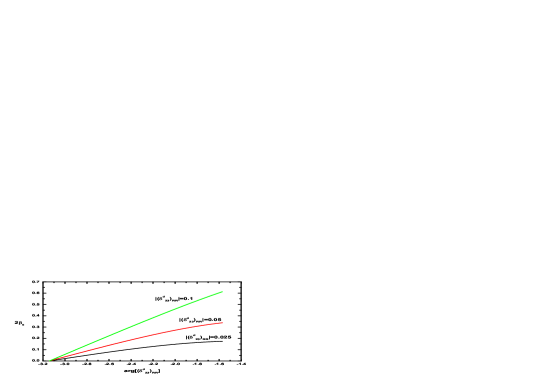
Figure 2: The $B^{0}_{s}-\bar{B}^{0}_{s}$ mixing phase as function of the $\arg[(\delta^{d}_{23})_{RR}]$ (in radians) for $|(\delta^{d}_{23})_{RR}|=0.025,0.05$ and $0.1$.

In Fig. 3, we present our results for the $B^{0}_{s}-\bar{B}^{0}_{s}$ mixing phase $2\beta_{s}$ as a function of $\arg[(\delta^{d}_{23})_{RR}]$ for $|(\delta^{d}_{23})_{RR}|=0.025,0.05$ and $0.1$. At these values the ratio $R$ is of order $\raise 1.29167pt\hbox{$\;<$\kern-7.5pt\raise-4.73611pt\hbox{$\sim\;$}}0.17,0.35$ and $0.7$ respectively. As can be seen from this figure, the values of $B^{0}_{s}$ mixing phase, which are consistent with the Hg EDM constraints, are typically of order $\raise 1.29167pt\hbox{$\;<$\kern-7.5pt\raise-4.73611pt\hbox{$\sim\;$}}0.1$. Therefore, one concludes that the SUSY contribution through the $B^{0}_{s}-\bar{B}^{0}_{s}$ mixing implies limited enhancement for $\sin 2\beta_{s}$ and thus cannot account for the new experimental results reported in Eq.(1,2). Moreover, a salient feature of this scenario with large $RR$ mixing is that it predicts a reachable mercury EDM in the future experiments.

5 SUSY contribution to $\bar{B}^{0}_{s}\to J/\psi\phi$ decay

In this section we will consider SUSY contribution to the decay $\bar{B}^{0}_{s}\to J/\psi\phi$. However, let us discuss the complexities in analyzing new physics effects in the decay amplitude for vector-vector final state[14].

Consider a $B\to V_{1}V_{2}$ decay which is dominated by a single weak decay amplitude within the SM. This holds for processes which are described by the quark-level decays ${\bar{b}}\to{\bar{c}}c{\bar{s}}$ which is the underlying quark transition in $\bar{B}^{0}_{s}\to J/\psi\phi$. In this case, the weak phase of the SM amplitude is zero in the standard parametrization [15]. Suppose now that there is a single dominant new physics amplitude, with a different weak phase, that contributes to the decay. This indeed will be the case for the SUSY contribution to $\bar{B}^{0}_{s}\to J/\psi\phi$. The decay amplitude for each of the three possible helicity states may be written as

$$A_{\lambda}\equiv{\rm Amp}(B\to V_{1}V_{2})_{\lambda} = a_{\lambda}e^{i\delta_{\lambda}^{a}}+b_{\lambda}e^{i\phi}e^{i\delta_{\lambda}^{b}}~{},$$

$${\bar{A}}_{\lambda}\equiv{\rm Amp}({\bar{B}}\to V_{1}V_{2})_{\lambda} = a_{\lambda}e^{i\delta_{\lambda}^{a}}+b_{\lambda}e^{-i\phi}e^{i\delta_{\lambda}^{b}}~{},$$ (53)

where $a_{\lambda}$ and $b_{\lambda}$ represent the SM and NP amplitudes, respectively, $\phi$ is the new-physics weak phase, the $\delta_{\lambda}^{a,b}$ are the strong phases, and the helicity index $\lambda$ takes the values $\left\{0,\|,\perp\right\}$. Using CPT invariance, the full decay amplitudes can be written as

$${\cal A} = {\rm Amp}(B\to V_{1}V_{2})=A_{0}g_{0}+A_{\|}g_{\|}+i\,A_{\perp}g_{\perp}~{},$$

$${\bar{\cal A}} = {\rm Amp}({\bar{B}}\to V_{1}V_{2})={\bar{A}}_{0}g_{0}+{\bar{A}}_{\|}g_{\|}-i\,{\bar{A}}_{\perp}g_{\perp}~{},$$ (54)

where the $g_{\lambda}$ are the coefficients of the helicity amplitudes written in the linear polarization basis. The $g_{\lambda}$ depend only on the angles describing the kinematics [16]. Eqs. (53) and (54) above enable us to write the time-dependent decay rates as

$$\Gamma(\bar{B}^{0}_{s}(t)\to V_{1}V_{2})=e^{-\Gamma t}\sum_{\lambda\leq\sigma}\Bigl{(}\Lambda_{\lambda\sigma}\pm\Sigma_{\lambda\sigma}\cos(\Delta Mt)\mp\rho_{\lambda\sigma}\sin(\Delta Mt)\Bigr{)}g_{\lambda}g_{\sigma}~{}.$$ (55)

Thus, by performing a time-dependent angular analysis of the decay $B(t)\to V_{1}V_{2}$, one can measure 18 observables. These are:

$$\Lambda_{\lambda\lambda}=\displaystyle\frac{1}{2}(|A_{\lambda}|^{2}+|{\bar{A}}_{\lambda}|^{2}),~{}~{} \Sigma_{\lambda\lambda}=\displaystyle\frac{1}{2}(|A_{\lambda}|^{2}-|{\bar{A}}_{\lambda}|^{2}),$$

$$\Lambda_{\perp i}=-\!{\rm Im}({A}_{\perp}{A}_{i}^{*}\!-\!{\bar{A}}_{\perp}{{\bar{A}}_{i}}^{*}), \Lambda_{\|0}={\rm Re}(A_{\|}A_{0}^{*}\!+\!{\bar{A}}_{\|}{{\bar{A}}_{0}}^{*}),$$

$$\Sigma_{\perp i}=-\!{\rm Im}(A_{\perp}A_{i}^{*}\!+\!{\bar{A}}_{\perp}{{\bar{A}}_{i}}^{*}), \Sigma_{\|0}={\rm Re}(A_{\|}A_{0}^{*}\!-\!{\bar{A}}_{\|}{{\bar{A}}_{0}}^{*}),$$

$$\rho_{\perp i}\!=\!{\rm Re}\!\Bigl{(}\frac{q}{p}\!\bigl{[}A_{\perp}^{*}{\bar{A}}_{i}\!+\!A_{i}^{*}{\bar{A}}_{\perp}\bigr{]}\Bigr{)}, \rho_{\perp\perp}\!=\!{\rm Im}\Bigl{(}\frac{q}{p}\,A_{\perp}^{*}{\bar{A}}_{\perp}\Bigr{)},$$

$$\rho_{\|0}\!=\!-{\rm Im}\!\Bigl{(}\frac{q}{p}[A_{\|}^{*}{\bar{A}}_{0}\!+\!A_{0}^{*}{\bar{A}}_{\|}]\Bigr{)}, \rho_{ii}\!=\!-{\rm Im}\!\Bigl{(}\frac{q}{p}A_{i}^{*}{\bar{A}}_{i}\Bigr{)},$$ (56)

where $i=\{0,\|\}$. In the above, $q/p$ is the weak phase factor associated with $B^{0}_{s}$-${\bar{B}}^{0}_{s}$ mixing. For $B^{0}_{s}$ meson, $q/p=\exp({-2\,i\beta_{s}})$. Note that $\beta_{s}$ may include NP effects in $B^{0}_{s}$-$\bar{B}^{0}_{s}$ mixing. Note also that the signs of the various $\rho_{\lambda\lambda}$ terms depend on the CP-parity of the various helicity states. We have chosen the sign of $\rho_{00}$ and $\rho_{\|\|}$ to be $-1$, which corresponds to the final state $J/\psi\phi$.

Not all of the 18 observables are independent. There are a total of six amplitudes describing $B\to V_{1}V_{2}$ and ${\bar{B}}\to V_{1}V_{2}$ decays [Eq. (53)]. Thus, at best one can measure the magnitudes and relative phases of these six amplitudes, giving 11 independent measurements.

The 18 observables given above can be written in terms of 13 theoretical parameters: three $a_{\lambda}$’s, three $b_{\lambda}$’s, $\beta_{s}$, $\phi$, and five strong phase differences defined by $\delta_{\lambda}\equiv\delta_{\lambda}^{b}-\delta_{\lambda}^{a}$, $\Delta_{i}\equiv\delta_{\perp}^{a}-\delta_{i}^{a}$. The explicit expressions for the observables can be found in Ref [14]. In the presence of new physics, one cannot extract the phase $\beta_{s}$. There are 11 independent observables, but 13 theoretical parameters. Since the number of measurements is fewer than the number of parameters, one cannot express any of the theoretical unknowns purely in terms of observables. In particular, it is impossible to extract $\beta_{s}$ cleanly.

In the absence of NP, the $b_{\lambda}$ are zero in Eq. (53). The number of parameters is then reduced from 13 to 6: three $a_{\lambda}$’s, two strong phase differences ($\Delta_{i}$), and $\beta_{s}$. It is straightforward to show that all six parameters can be determined cleanly in terms of the observables. This is exactly what is done in the experimental measurements to measure $\beta_{s}$, the value of which appears to be inconsistent with the SM. This might indicate new non SM phase in $B_{s}$ mixing or NP in the decay amplitude in which case the general angular analysis in Eq. (55) should be used. In the presence of NP, the indirect CP asymmetries for the various polarization states are not longer the same as it is in the SM( up to a sign).

In this section we will consider the scenario where SUSY gives significant contribution to both $B^{0}_{s}-\bar{B}^{0}_{s}$ mixing and the decay of $B^{0}_{s}\to J/\psi\phi$. In this case, the induced CP asymmetry is given by Eq.(25). As shown in Fig.(3), the SM the decay of $B^{0}_{s}\to J/\psi\phi$ takes place at tree level through the $b\to c$ transition. While the dominant SUSY contribution to this decay is given by the one loop level of gluino exchange for $b\to s$ transition. It is interesting to note that the SM amplitude is proportional to $G_{F}\times V_{bc}V_{cs}\sim 10^{-7}$, while the SUSY amplitude is given in terms of $\alpha_{s}^{2}/m_{\tilde{q}}^{2}\left((\delta^{d}_{LR})_{23}\times m_{\tilde{g}}/m_{b}\right)$. Therefore, although SUSY contribution is a loop level, it can be important relative to the SM one. In this respect, it is important to consider the impact of this contribution on the induced CP asymmetry $S^{\lambda}_{J/\psi\phi}$, as the phase of the mass insertion $(\delta^{d}_{LR})_{23}$ is not constrained by EDM.

Figure 3: SM tree level (left) and SUSY one loop (right) contributions to $\bar{B}^{0}_{s}\to J/\psi\phi$ decay.

Let us now write down the SM and SUSY contribution to $B^{0}_{s}(p)\to J/\psi(k_{1},\epsilon_{1})\phi(k_{2},\epsilon_{2})$, where we have labelled the momentum and polarization of the final state particles. To proceed with our calculation, we will first specify the momentum and polarization vectors of the final-state particles. We will work in the rest frame of the $B^{0}_{s}$ meson. We define the momentum and polarization of the vector $\phi$ meson as [17]

$$k_{2}^{\mu} = (E_{\phi},0,0,-k)$$

$$\varepsilon_{2}^{\mu}(0) = \frac{1}{m_{\phi}}(-k,0,0,E_{\phi})$$

$$\varepsilon_{2}^{\mu}(\mp) = \frac{1}{\sqrt{2}}(0,\mp 1,-i,0)~{},\$$ (57)

The momentum and polarization vectors for $J/\psi$ are defined as,

$$k_{1}^{\mu} = (E_{J/\psi},0,0,k)$$

$$\varepsilon_{1}^{\mu}(0) = \frac{1}{m_{J/\psi}}(k,0,0,E_{J/\psi})~{},$$

$$\varepsilon_{1}^{\mu}(\pm) = \frac{1}{\sqrt{2}}(0,\mp 1,-i,0)~{},\$$ (58)

The general amplitude for $\bar{B}^{0}_{s}(p)\to J/\psi(k_{1},\varepsilon_{1})\phi(k_{2},\varepsilon_{2})$, can be expressed as[18],

$$\bar{A}=\bar{a}\,\varepsilon_{1}^{*}\cdot\varepsilon_{2}^{*}+{\bar{b}\over m_{B_{s}}^{2}}(p\cdot\varepsilon_{1}^{*})(p\cdot\varepsilon_{2}^{*})+i{\bar{c}\over m_{B_{s}}^{2}}\epsilon_{\mu\nu\rho\sigma}p^{\mu}q^{\nu}\varepsilon_{1}^{*\rho}\varepsilon_{2}^{*\sigma}~{},$$ (59)

where $q=k_{1}-k_{2}$. For angular analysis it is useful to use the linear polarization basis. In this basis, one decomposes the decay amplitude into components in which the polarizations of the final-state vector mesons are either longitudinal ($A_{0}$), or transverse to their directions of motion and parallel ($A_{\|}$) or perpendicular ($A_{\perp}$) to one another. One writes [19, 20]

$$\bar{A}=\bar{A}_{0}\varepsilon_{1}^{*\scriptscriptstyle L}\cdot\varepsilon_{2}^{*\scriptscriptstyle L}-{1\over\sqrt{2}}\bar{A}_{\|}{\vec{\varepsilon}}_{1}^{*\scriptscriptstyle T}\cdot{\vec{\varepsilon}}_{2}^{*\scriptscriptstyle T}-{i\over\sqrt{2}}\bar{A}_{\perp}{\vec{\varepsilon}}_{1}^{*\scriptscriptstyle T}\times{\vec{\varepsilon}}_{2}^{*\scriptscriptstyle T}\cdot{\hat{p}}~{},$$ (60)

where ${\hat{p}}$ is the unit vector along the direction of motion of $V_{2}$ in the rest frame of $V_{1}$, $\varepsilon_{i}^{*\scriptscriptstyle L}={\vec{\varepsilon}}_{i}^{*}\cdot{\hat{p}}$, and ${\vec{\varepsilon}}_{i}^{*\scriptscriptstyle T}={\vec{\varepsilon}}_{i}^{*}-\varepsilon_{i}^{*\scriptscriptstyle L}{\hat{p}}$. $\bar{A}_{0}$, $\bar{A}_{\|}$, $\bar{A}_{\perp}$ are related to $a$, $b$ and $c$ of Eq. (59) via

$$\bar{A}_{\|}=\sqrt{2}\bar{a}~{},~{}~{}~{}\bar{A}_{0}=-\bar{a}x-{m_{1}m_{2}\over m_{\scriptscriptstyle B}^{2}}\bar{b}(x^{2}-1)~{},~{}~{}~{}\bar{A}_{\perp}=2\sqrt{2}\,{m_{1}m_{2}\over m_{\scriptscriptstyle B}^{2}}\bar{c}\sqrt{x^{2}-1}~{},$$ (61)

where $x=k_{1}\cdot k_{2}/(m_{1}m_{2})$. (A popular alternative basis is to express the decay amplitude in terms of helicity amplitudes $A_{\lambda}$, where $\lambda=1,0,-1$ [21, 19]. The helicity amplitudes can be written in terms of the linear polarization amplitudes via $A_{\pm 1}=(A_{\|}\pm A_{\perp})/\sqrt{2}$, with $A_{0}$ the same in both bases.)

We will now proceed to calculate the polarization dependent CP asymmetry given in Eq. 25. We will use factorization to calculate the ratio $r_{A}^{\lambda}=|A_{{\rm NP}}^{\lambda}/A_{{\rm SM}}^{\lambda}|$. In factorization there are no strong phases and we will keep them as a free unknown parameter in the expression for $S_{J/\psi\phi}^{\lambda}$ in Eq. (25). The amplitude for the process $\bar{B}_{s}(p)\to J/\psi(k_{1},\varepsilon_{1})\phi(k_{2},\varepsilon_{2})$, in the SM, is given by,

$$\bar{A}[\bar{B}_{s}\to J/\psi\phi]=\frac{G_{F}}{\sqrt{2}}XL_{J/\psi},$$ (62)

with

$$X = V_{cb}V_{cs}^{*}a_{2}-\sum_{q=u,c,t}V_{qb}V_{qs}^{*}(a_{3}^{q}+a_{5}^{q}+a_{7}^{q}+a_{9}^{q})~{},$$

$$L_{J/\psi} = m_{J/\psi}g_{J/\psi}\varepsilon_{1}^{*\mu}\left\langle\phi\right|\bar{s}\gamma_{\mu}(1-\gamma_{5})b\left|\bar{B}_{s}\right\rangle,\ ~{}.$$ (63)

where $a_{2}=c_{2}+\frac{c_{1}}{N_{c}}$ and for $i>2$, $a_{i}=c_{i}+\frac{c_{i+i}}{N_{c}}$, with $c_{i}$ being the Wilson’s coefficient. Here $g_{J/\psi}$ is the $J/\psi$ decay constant defined in the usual manner.

We can simplify $X$ using several facts. First $a_{2}$ is much larger than $a_{i}^{t}$ with $i=3,5,7,9$ [22]. Second, in the penguin contributions in Eq. (63) we have included the rescattering contributions from the tree operators. However these are small and the contributions $a_{3}^{u,c}$ and $a_{5}^{u,c}$ due to perturbative QCD rescattering vanish because of the following relations,

$$c_{3,5}^{u,c} = -c_{4,6}^{u,c}/N_{c}=P^{u,c}_{s}/N_{c}\;,\;\;$$ (64)

where $N_{c}$ is the number of color. The leading contributions to $P^{i}_{s}$ are given by: $P^{i}_{s}=({\frac{\alpha_{s}}{8\pi}})c_{1}({\frac{10}{9}}+G(m_{i},\mu,q^{2}))$ with $i=u,c$. The function $G(m,\mu,q^{2})$ is given by

$$G(m,\mu,q^{2})=4\int^{1}_{0}x(1-x)\mbox{ln}{m^{2}-x(1-x)q^{2}\over\mu^{2}}~{}\mbox{d}x\;.$$ (65)

The rescattering via electroweak interactions are given by [23]

$$c_{7,9}^{u,c}=P^{u,c}_{e}\;,\;\;c_{8,10}^{u,c}=0$$ (66)

with $P^{i}_{e}=({\frac{\alpha_{em}}{9\pi}})(N_{c}c_{2}+c_{1})({\frac{10}{9}}+G(m_{i},\mu,q^{2}))$. These contributions are again much smaller than the dominant tree contributions and can be neglected.

In light of the above facts we can conclude that the dominant contributions in $X$ in Eq. (63) come the tree level term where $c_{1}=1.081$ and $c_{2}=-0.190$ are the relevant Wilson coefficients [22]. This leads to

$$X \approx V_{cb}V_{cs}^{*}a_{2}=0.17V_{cb}V_{cs}^{*}\$$ (67)

The matrix elements in Eq. (63) above can be expressed in terms of form factors. This can be done as follows [24]:

$$\left\langle V_{2}(k_{2})\right|{\bar{q}}^{\prime}\gamma_{\mu}b\left|\bar{B}_{s}(p)\right\rangle = i{{2V^{(2)}(r^{2})}\over(m_{B}+m_{2})}\epsilon_{\mu\nu\rho\sigma}p^{\nu}k_{2}^{\rho}\varepsilon_{2}^{*\sigma}~{},$$

$$\left\langle V_{2}(k_{2})\right|{\bar{q}}^{\prime}\gamma_{\mu}\gamma_{5}b\left|B(p)\right\rangle = (m_{B}+m_{2})A_{1}^{(2)}(r^{2})\left[\varepsilon_{2\mu}^{*}-\frac{\varepsilon_{2}^{*}.r}{r^{2}}r_{\mu}\right]$$ (68)

$$~{}-A_{2}^{(2)}(r^{2})\frac{\varepsilon_{2}^{*}.r}{m_{B}+m_{2}}\left[(p_{\mu}+k_{2\mu})-\frac{m_{B}^{2}-m_{2}^{2}}{r^{2}}r_{\mu}\right]$$

$$~{}+2im_{2}\frac{\varepsilon_{2}^{*}.r}{r^{2}}r_{\mu}A_{0}^{(2)}(r^{2})~{},$$

where $r=p-k_{2}$, and $V^{(2)}$, $A_{1}^{(2)}$, $A_{2}^{(2)}$ and $A_{0}^{(2)}$ are form factors.

Using Eq. (68) in Eq. (63) one obtains,

$$\bar{a}_{SM} = -\frac{G_{F}}{\sqrt{2}}m_{J/\psi}g_{J/\psi}x(m_{B_{s}}+m_{\phi})A_{1}^{(2)}(m_{J/\psi}^{2})X$$

$$\bar{b}_{SM} = \frac{G_{F}}{\sqrt{2}}2m_{J/\psi}g_{J/\psi}{m_{B_{s}}\over(m_{B_{s}}+m_{\phi})}m_{B_{s}}A_{2}^{(2)}(m_{J/\psi}^{2})X$$

$$\bar{c}_{SM} = -\frac{G_{F}}{\sqrt{2}}m_{J/\psi}g_{J/\psi}{m_{B_{s}}\over(m_{B_{s}}+m_{\phi})}m_{B_{s}}V^{(2)}(m_{J/\psi}^{2})X.\$$ (69)

Let us turn now to the SUSY contribution. We will consider only the dominanat chromomagnetic operators. The gluon in these operators can split into a charm quark pair, thereby contributing to $b\to s\bar{c}c$. We begin with a discussion on the matrix elements of the chromomagnetic operators $O_{g}$ and $\widetilde{O}_{g}$. These are given by,

$$\langle J/\psi\phi|O_{g}|{\bar{B}_{s}}\rangle = <O_{g}>$$

$$= -\frac{\alpha_{s}m_{b}}{\pi q^{2}}\langle J/\psi\phi|\left(\bar{s}_{\alpha}\gamma_{\mu}{\not{q}}(1+\gamma_{5})\frac{\lambda^{A}_{\alpha\beta}}{2}b_{\beta}\right)\left(\bar{s}_{\rho}\gamma^{\mu}\frac{\lambda^{A}_{\rho\sigma}}{2}s_{\sigma}\right)|{\bar{B}_{s}}\rangle$$

$$\langle J/\psi\phi|\widetilde{O}_{g}|{\bar{B}_{s}}\rangle = <\widetilde{O}_{g}>$$

$$= -\frac{\alpha_{s}m_{b}}{\pi q^{2}}\langle J/\psi\phi|\left(\bar{s}_{\alpha}\gamma_{\mu}{\not{q}}(1-\gamma_{5})\frac{\lambda^{A}_{\alpha\beta}}{2}b_{\beta}\right)\left(\bar{s}_{\rho}\gamma^{\mu}\frac{\lambda^{A}_{\rho\sigma}}{2}s_{\sigma}\right)|{\bar{B}_{s}}\rangle$$

(70)

where $q^{\mu}$ is the momentum carried by the gluon in the penguin diagram. In our case $q^{\mu}$ coincides with the four momentum of the $J/\psi$.

After a color fierz we can write the operator $O_{g}$ as,

$$O_{g} = Y_{g}\left[-\frac{2}{N_{c}}\left(\bar{s}_{\alpha}\gamma_{\mu}\frac{{\not{q}}}{m_{b}}(1+\gamma_{5})b_{\alpha}\right)\left(\bar{s}_{\beta}\gamma^{\mu}s_{\beta}\right)+..\right]$$

$$\widetilde{O}_{g} = Y_{g}\left[-\frac{2}{N_{c}}\left(\bar{s}_{\alpha}\gamma_{\mu}\frac{{\not{q}}}{m_{b}}(1-\gamma_{5})b_{\alpha}\right)\left(\bar{s}_{\beta}\gamma^{\mu}s_{\beta}\right)+..\right]$$

$$Y_{g} = -\frac{\alpha_{s}m_{b}^{2}}{4\pi m_{J/\psi}^{2}}.\$$

In the above we have only retained terms that contribute to the decay $\bar{B}_{s}(p)\to J/\psi(k_{1},\varepsilon_{1})\phi(k_{2},\varepsilon_{2})$ In factorization, after using equation of motion, we can write the matrix element of $O_{g}$ as,

$$<O_{g}> = T_{1}+T_{2}+T_{3}$$

$$T_{1} = C_{g}Y_{g}\left[-\frac{2}{N_{c}}L_{J/\psi}\right]$$

$$L_{J/\psi} = m_{J/\psi}g_{J/\psi}\varepsilon_{1}^{*\mu}\left\langle\phi\right|\bar{s}\gamma_{\mu}(1-\gamma_{5})b\left|\bar{B}_{s}\right\rangle,$$

$$T_{2} = C_{g}Y_{g}\frac{m_{s}}{m_{b}}\left[-\frac{2}{N_{c}}R_{J/\psi}\right]$$

$$R_{J/\psi} = m_{J/\psi}g_{J/\psi}\varepsilon_{1}^{*\mu}\left\langle\phi\right|\bar{s}\gamma_{\mu}(1+\gamma_{5})b\left|\bar{B}_{s}\right\rangle,$$

$$T_{3} = C_{g}Y_{g}\frac{2\varepsilon_{1}^{*}\cdot k_{2}}{m_{b}}\left[\frac{2}{N_{c}}S_{J/\psi}\right]$$

$$S_{J/\psi} = m_{J/\psi}g_{J/\psi}\left\langle\phi\right|\bar{s}(1+\gamma_{5})b\left|\bar{B}_{s}\right\rangle.\$$ (71)

In the above $m_{s,b}$ are the strange and the bottom quark masses.

In the above equation it is clear that $T_{2}$ is suppressed relative to $T_{1}$ by ${m_{s}\over m_{b}}$ and we will neglect it. From the structure of the polarization vectors in Eq. (57), it is also clear that the $\pm$ polizations do not contribute to $T_{3}$. Hence for the $\pm$ polarizations we can obtain a clear prediction for $r^{\lambda}_{A}$ defined below Eq. (25), as the form factors and other hadronic quantities cancel in the ratio.

For the matrix element of the operator $\widetilde{O}_{g}$, focussing only on the transverse amplitues we can write,

$$<\widetilde{O}_{g}> = Y_{g}\left[-\frac{2}{N_{c}}R_{J/\psi}\right]$$

$$R_{J/\psi} = m_{J/\psi}g_{J/\psi}\varepsilon_{1}^{*\mu}\left\langle\phi\right|\bar{s}\gamma_{\mu}(1+\gamma_{5})b\left|\bar{B}_{s}\right\rangle,\$$ (72)

Hence again focussing only on the transverse amplitudes we can write, using Eq. (68) in Eq. (71) and Eq. (72),

$$\bar{a}_{susy} = -\frac{G_{F}}{\sqrt{2}}m_{J/\psi}g_{J/\psi}(m_{B_{s}}+m_{\phi})A_{1}^{(2)}(m_{J/\psi}^{2})(Y-\tilde{Y})$$

$$\bar{c}_{susy} = -\frac{G_{F}}{\sqrt{2}}m_{J/\psi}g_{J/\psi}{m_{B_{s}}\over(m_{B_{s}}+m_{\phi})}m_{B_{s}}V^{(2)}(m_{J/\psi}^{2})(Y+\tilde{Y})$$

$$Y = \frac{\sqrt{2}C_{g}}{G_{F}}Y_{g}\left[-\frac{2}{N_{c}}\right]$$

$$\widetilde{Y} = \frac{\sqrt{2}\widetilde{C_{g}}}{G_{F}}Y_{g}\left[-\frac{2}{N_{c}}\right]$$

$$Y_{g} = -\frac{\alpha_{s}m_{b}^{2}}{4\pi m_{J/\psi}^{2}}\$$ (73)

Combining the SM and SUSY contributions we can now compute,

$$r_{A}^{\|} = |A_{{\rm NP}}^{\|}/A_{{\rm SM}}^{\|}|=|\frac{(Y-\widetilde{Y})}{X}|$$

$$r_{A}^{\perp} = |A_{{\rm NP}}^{\perp}/A_{{\rm SM}}^{\perp}|=|\frac{(Y+\widetilde{Y})}{X}|\$$ (74)

Using the values of $V_{cb}$ and $V_{cs}$ from Ref [15] we obtain $X\approx 0.0069$. Futhermore with $m_{\widetilde{g}}=m_{\widetilde{q}}=500$ GeV, $m_{b}(m_{b})=4.5$ GeV, we obtain,

$$Y \approx =2.1315(\delta^{d}_{LR})_{23}\left[\frac{-2}{N_{c}}Y_{g}\right]=0.0477(\delta^{d}_{LR})_{23}$$

$$\widetilde{Y} \approx =2.1315(\delta^{d}_{RL})_{23}\left[\frac{-2}{N_{c}}Y_{g}\right]=0.0477(\delta^{d}_{RL})_{23}\$$ (75)

We can then write, using Eq. 74,

$$r_{A}^{\|} \approx 0.07\frac{\sqrt{(|(\delta^{d}_{LR})_{23}|)^{2}+(|(\delta^{d}_{RL})_{23}|)^{2}-2|(\delta^{d}_{LR})_{23}||(\delta^{d}_{RL})_{23}|\cos(\theta_{LR}-\theta_{RL})}}{0.01}$$

$$r_{A}^{\perp} \approx 0.07\frac{\sqrt{(|(\delta^{d}_{LR})_{23}|)^{2}+(|(\delta^{d}_{RL})_{23}|)^{2}+2|(\delta^{d}_{LR})_{23}||(\delta^{d}_{RL})_{23}|\cos(\theta_{LR}-\theta_{RL})}}{0.01},\$$ (76)

where $\theta_{LR}$ and $\theta_{RL}$ are the phases of $(\delta^{d}_{LR})_{23}$ and $(\delta^{d}_{RL})_{23}$. We will set $|(\delta^{d}_{LR})_{23}|=|(\delta^{d}_{RL})_{23}|=0.01$ and we can then now consider the following cases:

Case a $(\delta^{d}_{LR})_{23}=(\delta^{d}_{RL})_{23}$. In this case we obtain,

$$S_{J/\psi\phi}^{\|} = \sin(2\beta_{s}^{SM}+2\theta_{s})$$

$$S_{J/\psi\phi}^{\perp} = \sin(2\beta_{s}^{SM}+2\theta_{s})+0.28\cos(2\beta_{s}^{SM}+2\theta_{s})\sin\theta^{\perp}_{{\rm NP}}\cos\delta^{\perp}.\$$ (77)

If we neglect the contribution from mixing then $S_{J/\psi\phi}^{\perp}$ can reach a value of upto 0.3 for $\sin\theta^{\perp}_{{\rm NP}}\sim 1$ and $\cos\delta^{\perp}\sim 1$.

Case b $(\delta^{d}_{LR})_{23}=-(\delta^{d}_{RL})_{23}$. In this case we obtain,

$$S_{J/\psi\phi}^{\|} = \sin(2\beta_{s}^{SM}+2\theta_{s})+0.28\cos(2\beta_{s}^{SM}+2\theta_{s})\sin\theta^{\|}_{{\rm NP}}\cos\delta^{\|}$$

$$S_{J/\psi\phi}^{\perp} = \sin(2\beta_{s}^{SM}+2\theta_{s}).\$$ (78)

Again, if we neglect the contribution from mixing then $S_{J/\psi\phi}^{\|}$ can reach a value of upto 0.3 for $\sin\theta^{\|}_{{\rm NP}}\sim 1$ and $\cos\delta^{\|}\sim 1$. Finally, we can consider the case where either $(\delta^{d}_{LR})_{23}$ or $(\delta^{d}_{RL})_{23}$ is zero. For the case $(\delta^{d}_{LR})_{23}\neq 0,(\delta^{d}_{RL})_{23}=0$ we obtain,

$$S_{J/\psi\phi}^{\|} = \sin(2\beta_{s}^{SM}+2\theta_{s})+0.14\cos(2\beta_{s}^{SM}+2\theta_{s})\sin\theta^{\|}_{{\rm NP}}\cos\delta^{\|}$$

$$S_{J/\psi\phi}^{\perp} = \sin(2\beta_{s}^{SM}+2\theta_{s})+0.14\cos(2\beta_{s}^{SM}+2\theta_{s})\sin\theta^{\perp}_{{\rm NP}}\cos\delta^{\perp}\$$ (79)

For the case $(\delta^{d}_{LR})_{23}=0,(\delta^{d}_{RL})_{23}\neq 0$ we obtain,

$$S_{J/\psi\phi}^{\|} = \sin(2\beta_{s}^{SM}+2\theta_{s})-0.14\cos(2\beta_{s}^{SM}+2\theta_{s})\sin\theta^{\|}_{{\rm NP}}\cos\delta^{\|}$$

$$S_{J/\psi\phi}^{\perp} = \sin(2\beta_{s}^{SM}+2\theta_{s})+0.14\cos(2\beta_{s}^{SM}+2\theta_{s})\sin\theta^{\perp}_{{\rm NP}}\cos\delta^{\perp}\$$ (80)

Now one may wonder how NP in $b\to s\bar{c}c$ transitions affect CP measurements in the $B_{d}$ system. Let us first consider the indirect CP asymmetry in the golden mode $B_{d}\to J/\psi K_{s}$. Note this is a vector-pseudoscalar decay and so the strong phases involved here can be quite different from the ones involved in vector-vector decays. In other words NP effects in different final states can be very different. More interestingly, it can be easily checked that for case b in Eq. (78) the contribution to the indirect asymmetry in $B_{d}\to J/\psi K_{s}$ cancels. However, the indirect CP asymmetry in the vector-vector mode does not cancel for all polarization states. In other words the range of NP effects obtained in the decay $B_{s}\to J/\psi\phi$ are consistent with $\sin{2\beta}$ measurements in $B_{d}\to J/\psi K_{s}$ [25, 26, 27] for the various reasons discussed above.

The decay $B_{d}\to J/\psi K*$ is related to $B^{0}_{s}\to J/\psi\phi$ by $SU(3)$ flavor symmetry. Hence we should potentially see NP effects in $B_{d}\to J/\psi K*$ , up to $SU(3)$ breaking effects. The CP measurements in this decay are not yet precise [25] and hence this decay also is an ideal place to look for new physics effects in the decay amplitude.

5.1 Summary

In summary, we have analyzed the SUSY contribution to $B^{0}_{s}-\bar{B}^{0}_{s}$ mixing in light of recent experimental measurement of the mixing phase. We showed that the experimental limits of the mass difference $\Delta M_{B_{s}}$ and the mercury EDM constrain significantly the SUSY contribution to $B^{0}_{s}-\bar{B}^{0}_{s}$ mixing, so that $\sin 2\beta_{s}\raise 1.29167pt\hbox{$\;<$\kern-7.5pt\raise-4.73611pt\hbox{$\sim\;$}}0.1$. We then studied the the one loop SUSY contribution to $B^{0}_{s}\to J/\psi\phi$ decay and found that new physics contribution to the decay amplitude can lead to significant indirect CP asymmetries which are in general different for different polarization states.

References

[1]
T. Aaltonen et al. [CDF Collaboration],
Phys. Rev. Lett. 100, 161802 (2008)
[arXiv:0712.2397 [hep-ex]].
[2]
V. M. Abazov et al. [D0 Collaboration],
Phys. Rev. Lett. 101, 241801 (2008)
[arXiv:0802.2255 [hep-ex]].
[3]
M. Bona et al. [UTfit Collaboration],
arXiv:0803.0659 [hep-ph].
[4]
S. Abel, S. Khalil and O. Lebedev,
Nucl. Phys. B 606, 151 (2001)
[arXiv:hep-ph/0103320].
[5]
S. Khalil and E. Kou,
Phys. Rev. D 67, 055009 (2003)
[arXiv:hep-ph/0212023].
[6]
S. Khalil and E. Kou,
Phys. Rev. Lett. 91, 241602 (2003)
[arXiv:hep-ph/0303214].
[7]
S. Khalil,
Phys. Rev. D 72, 035007 (2005)
[arXiv:hep-ph/0505151].
[8]
S. Baek, P. Hamel, D. London, A. Datta and D. A. Suprun,
Phys. Rev. D 71, 057502 (2005)
[arXiv:hep-ph/0412086];
A. Datta, M. Imbeault, D. London, V. Page, N. Sinha and R. Sinha,
Phys. Rev. D 71, 096002 (2005)
[arXiv:hep-ph/0406192];
A. Datta and D. London,
Phys. Lett. B 595, 453 (2004)
[arXiv:hep-ph/0404130].
[9]
P. Ball, S. Khalil and E. Kou,
Phys. Rev. D 69, 115011 (2004)
[arXiv:hep-ph/0311361].
[10]
F. Gabbiani, E. Gabrielli, A. Masiero and L. Silvestrini,
Nucl. Phys. B 477 (1996) 321 [arXiv:hep-ph/9604387].
[11]
D. Becirevic et al.,
Nucl. Phys. B 634 (2002) 105 [arXiv:hep-ph/0112303].
[12]
J. Hisano and Y. Shimizu,
Phys. Rev. D 70, 093001 (2004)
[arXiv:hep-ph/0406091].
[13]
S. Abel and S. Khalil,
Phys. Lett. B 618, 201 (2005)
[arXiv:hep-ph/0412344].
[14]
D. London, N. Sinha and R. Sinha,
Phys. Rev. D 69, 114013 (2004)
[arXiv:hep-ph/0402214];
D. London, N. Sinha and R. Sinha,
Europhys. Lett. 67, 579 (2004)
[arXiv:hep-ph/0304230].
[15]
C. Amsler et al., Physics Letters B667, 1 (2008).
[16] N. Sinha and R. Sinha, Phys. Rev. Lett. 80, 3706 (1998);
A.S. Dighe, I. Dunietz and R. Fleischer, Eur. Phys. J. C6, 647, (1999).
[17]
A. Datta, Y. Gao, A. V. Gritsan, D. London, M. Nagashima and A. Szynkman,
Phys. Rev. D 77, 114025 (2008)
[arXiv:0711.2107 [hep-ph]].
[18]
A. Datta and D. London,
Int. J. Mod. Phys. A 19, 2505 (2004)
[arXiv:hep-ph/0303159].
[19] A.S. Dighe, I. Dunietz, H.J. Lipkin and J.L. Rosner,
Phys. Lett. 369B, 144 (1996); B. Tseng and C.-W. Chiang, hep-ph/9905338.
[20] N. Sinha and R. Sinha, Phys. Rev. Lett. 80, 3706 (1998); C.-W. Chiang
and L. Wolfenstein, Phys. Rev. D61, 074031 (2000).
[21] G. Kramer and W.F. Palmer, Phys. Rev. D45, 193 (1992),
Phys. Lett. 279B, 181 (1992), Phys. Rev. D46, 2969 (1992); G. Kramer, W.F. Palmer
and T. Mannel, Zeit. Phys. C55, 497 (1992); G. Kramer, W.F. Palmer and
H. Simma, Nucl. Phys. B428, 77 (1994); A.N. Kamal and C.W. Luo,
Phys. Lett. 388B, 633 (1996); D. Atwood and A. Soni, Phys. Rev. Lett. 81, 3324 (1998),
Phys. Rev. D59, 013007 (1999).
[22] See, for example, G. Buchalla, A.J. Buras and
M.E. Lautenbacher, Rev. Mod. Phys.68, 1125 (1996).
[23]
T. E. Browder, A. Datta, X. G. He and S. Pakvasa,
Phys. Rev. D 57, 6829 (1998)
[arXiv:hep-ph/9705320].
[24] M. Bauer, B. Stech and M, Wirbel, Zeit. Phys. C34, 103 (1987).
[25]
E. Barberio et al. [Heavy Flavor Averaging Group],
arXiv:0808.1297 [hep-ex].
[26]
UTFit: Unitarity Triangle Fit to CKM Matrix.
http://www.utfit.org/
[27]
CKMfitter Group (J. Charles et al.),
Eur. Phys. J. C41, 1-131 (2005) [hep-ph/0406184],
updated results and plots available at: http://ckmfitter.in2p3.fr