N to $\Delta$ transition amplitudes from QCD sum rules

Abstract

We present a calculation of the N to $\Delta$ electromagnetic transition amplitudes using the method of QCD sum rules. A complete set of QCD sum rules is derived for the entire family of transitions from the baryon octet to decuplet. They are analyzed in conjunction with the corresponding mass sum rules using a Monte-Carlo-based analysis procedure. The performance of each of the sum rules is examined using the criteria of OPE convergence and ground-state dominance, along with the role of the transitions in intermediate states. Individual contributions from the u, d and s quarks are isolated and their implications in the underlying dynamics are explored. Valid sum rules are identified and their predictions are obtained. The results are compared with experiment and other calculations.

I Introduction

The determination of low-energy electromagnetic properties of baryons, such as charge radii, magnetic and quadrupole moments, has long been a subject of interest in nucleon structure studies. For example, the E2/M1 ratio of the transition amplitudes in the process $\gamma N\rightarrow\Delta$ is a signature of the deviation of the nucleon from spherical symmetry.

The first serious attempt to determine the ratio from quantum chromodynamics (QCD), the fundamental theory of the strong interaction, was the lattice calculation of Leinweber et al. Derek93 . The calculation has been updated recently by Alexandrou et al. alex04 ; alex08 with better technology and statistics. In this work, we present a calculation of the transition amplitudes using the SVZ method of QCD sum rules SVZ79 which is another nonperturbative approach firmly-entrenched in QCD with minimal modeling. The approach provides a general way of linking hadron phenomenology with the interactions of quarks and gluons via only a few parameters: the QCD vacuum condensates and susceptibilities. The analytic nature of the approach offers an unique perspective on how the properties of hadrons arise from nonperturbative interactions in the QCD vacuum, and gives a complimentary view of the same physics to the numerical approach of lattice QCD. It has been successfully applied to almost every aspect of strong-interaction physics, including the only other attempt on the N to $\Delta$ transition that we know of by Ioffe Ioffe84 over 25 years ago. It was a limited study conducted in the context of the magnetic moments of the nucleon, and the results were inconclusive due to large contamination from the excited-state contributions.

The above discussion only concerns with the classic QCD sum rule method by SVZ. There are a number of studies on N to $\Delta$ transitions in the so-called light cone QCD sum rule method (or LCSR) Rohrwild07 ; Aliev06 . The main difference is that it employs as input light-cone wavefunctions, instead of vacuum condensates. One advantage of the light-cone QCD method is that one can compute the transition form factor at non-zero momentum transfer relatively easily Belyaev96 ; Braun06 .

Our goal is to carry out a comprehensive study of the N to $\Delta$ transition in the SVZ QCD sum rule method with a number of features. First, we employ generalized interpolating fields which allow us to use the optimal mixing of interpolating fields to achieve the best match in the QCD sum rules. The interpolating field used previously is a special case. Second, we derive the complete tensor structure and construct a new set of QCD sum rules. The previous study was quite limited in its tensor structure. Third, we study all tranisitons from the octet to te deuplet, not just the proton channel. Fourth, we perform a Monte-Carlo uncertainty analysis which has become the standard for evaluating errors in the QCD sum rule approach. The advantage of such an analysis is explained later. Fifth, we use a different procedure to extract the transition amplitudes and to treat the transition terms in the intermediate states. Our results show that these transitions cannot be simply ignored. Sixth, we isolate the individual quark contributions to the transition amplitudes and discuss their implications in the underlying quark-gluon dynamics. A similar study has been performed for the magnetic moments of octet baryons Wang08 .

The paper is organized as follows. In Section II, the physics of N to $\Delta$ transition is reviewed. In Section III, the external field method of QCD sum rules is applied to this process. Master formulas are calculated using the full sets of interpolating fields for the octet and decuplet baryons. Then the full phenomenological representation and QCD side are calculated, leading to a complete set of QCD sum rules for the entire family of transitions from the octet to the decuplet. Section IV describes our numerical procedure to extract the transition amplitudes. Section V summarizes the results and gives a comparison of our results with experiment and other calculations. The conclusions are given in Section VI.

II Physics of N to $\Delta$ transitions

II.1 Definition of the form factors

The concept of form factors plays an important role in the study of internal structure of composite particles. The non-trivial dependence of form factors on the momentum transfer (i.e., its deviation from the constant behavior) is a signal of the non-elementary nature of the investigated particle. The current matrix element for the $\gamma N\to\Delta$ transition can be written as

$$<\Delta(k^{\prime},s^{\prime})|j_{\mu}|N(k,s)>=\bar{u}^{\rho}(k^{\prime},s^{\prime})\Gamma_{\rho\mu}u(k,s),$$ (1)

where $k,s$ and $k^{\prime},s^{\prime}$ denote initial and final momenta and spins, $j_{\mu}$ the electromagnetic current, $u$ the spin-1/2 nucleon spinor, and $u^{\rho}$ the Rarita-Schwinger spinor for the spin-3/2 $\Delta$. This matrix element is the most general form required for describing on-shell nucleon and $\Delta$ states with both real and virtual photons. There exist different definitions in the literature for the form factors describing the vertex function $\Gamma_{\rho\mu}$. One is in terms of $G_{1}$, $G_{2}$, and $G_{3}$ by Jones-Scadron JS73 :

$$\Gamma_{\rho\mu}=G_{1}(q^{2}){\rm H}_{\rho\mu}^{1}+G_{2}(q^{2}){\rm H}_{\rho\mu}^{2}+G_{3}(q^{2}){\rm H}_{\rho\mu}^{3},$$ (2)

where the invariant structures are

$$\begin{array}[]{rcl}H_{\rho\mu}^{1}&=&q_{\rho}\gamma_{\mu}-q\cdot\gamma g_{\rho\mu};\\ H_{\rho\mu}^{2}&=&q_{\rho}P_{\mu}-q\cdot Pg_{\rho\mu};\\ H_{\rho\mu}^{3}&=&q_{\rho}q_{\mu}-q^{2}g_{\rho\mu}.\end{array}$$ (3)

Here $q=k^{\prime}-k$ is the four-momentum transfer. For real photons ($q^{2}=0$), only $G_{1}(0)$ and $G_{2}(0)$ play a role. Note that the form factors defined this way are dimensionful: $G_{1}$ in GeV^-1, $G_{2}$ in GeV^-2, and $G_{3}$ in GeV^-3. They are analogous to the Pauli-Dirac form factors $F_{1}$ and $F_{2}$ for the nucleon.

Another definition commonly used in lattice QCD calculations Derek93 ; alex04 is

$$\begin{array}[]{l}<\Delta(k^{\prime},s^{\prime})|j^{\mu}|N(k,s)>\\ =i\sqrt{\frac{2}{3}}\left(m_{\Delta}m_{N}\over E_{\Delta}E_{N}\right)^{1/2}\bar{u}_{\rho}(k^{\prime},s^{\prime})\Gamma^{\rho\mu}u(k,s),\end{array}$$ (4)

where

$$\Gamma^{\rho\mu}=G_{M1}(q^{2})K_{M1}^{\rho\mu}+G_{E2}(q^{2})K_{E2}^{\rho\mu}+G_{C2}(q^{2})K_{C2}^{\rho\mu},$$ (5)

in terms of the magnetic dipole $G_{M1}$, electric quadrupole $G_{E2}$, and Coulomb quadrupole $G_{C2}$ form factors. They are analogous to the Sachs form factors $G_{E}$ and $G_{M}$ for the nucleon. The invariant functions involve the masses of the particles explicitly,

$$\begin{array}[]{rcl}K_{M1}^{\rho\mu}&=&-\frac{3}{{(m_{\Delta}+m_{N})^{2}+q^{2}}}\frac{{(m_{\Delta}+m_{N})}}{{2m_{N}}}\varepsilon^{\rho\mu\alpha\beta}P_{\alpha}q_{\beta};\\ K_{E2}^{\rho\mu}&=&-K_{M1}^{\rho\mu}-6\Omega^{-1}(q^{2})\varepsilon^{\rho\lambda\alpha\beta}P_{\alpha}q_{\beta}{\varepsilon^{\mu}\lambda}^{\gamma\delta}(2P_{\gamma}+q_{\gamma})\\ &&\times q_{\delta}i\gamma_{5}\frac{{(m_{\Delta}+m_{N})}}{{2m_{N}}};\\ K_{C2}^{\rho\mu}&=&-6\Omega^{-1}(q^{2})q^{\rho}(q^{2}P^{\mu}-q\cdot Pq^{\mu})i\gamma_{5}\frac{{(m_{\Delta}+m_{N})}}{{2m_{N}}},\\ \end{array}$$ (6)

where $P=(k^{\prime}+k)/2$ and $\Omega(q^{2})=[(m_{\Delta}+m_{N})^{2}-q^{2}][(m_{\Delta}-m_{N})^{2}-q^{2}]$.

We stress that the two sets of form factors are equivalent in describing the physics of N to $\Delta$ transitions. They are related by

$$\begin{array}[]{rcl}G_{M1}(Q^{2})&=&\frac{{m_{N}}}{{3(m_{N}+m_{\Delta})}}[((3m_{\Delta}+m_{N})(m_{\Delta}+m_{N})+Q^{2})\\ &&\frac{{G_{1}(Q^{2})}}{{m_{\Delta}}}+(m_{\Delta}^{2}-m_{N}^{2})G_{2}(Q^{2})-2Q^{2}G_{3}(Q^{2})];\\ G_{E2}(Q^{2})&=&\frac{{m_{N}}}{{3(m_{N}+m_{\Delta})}}[(m_{\Delta}^{2}-m_{N}^{2}-Q^{2})\frac{{G_{1}(Q^{2})}}{{m_{\Delta}}}\\ &&+(m_{\Delta}^{2}-m_{N}^{2})G_{2}(Q^{2})-2Q^{2}G_{3}(Q^{2})];\\ G_{C2}(Q^{2})&=&\frac{{2m_{N}}}{{3(m_{\Delta}+m_{N})}}[2m_{\Delta}G_{1}(Q^{2})+\frac{1}{2}(3m_{\Delta}^{2}+m_{N}^{2}+Q^{2})\\ &&G_{2}(Q^{2})+(m_{\Delta}^{2}-m_{N}^{2}-Q^{2})G_{3}(Q^{2})].\end{array}$$ (7)

Here we have switched to the notation of $Q^{2}=-q^{2}$ since most studies of form factors are for space-like momentum transfers ($q^{2}<0$ or $Q^{2}>0$). The inverse form, omitting the explicit $Q^{2}$ dependence in the G’s, is given as:

$$\begin{array}[]{rcl}G_{1}&=&-{3(G_{E2}-G_{M1})[m_{\Delta}(m_{\Delta}+m_{N})]}\\ &&/{[2m_{N}((m_{\Delta}+m_{N})^{2}+Q^{2})]};\\ G_{2}&=&-3(m_{\Delta}+m_{N})[(-2G_{C2}Q^{2}\\ &&+G_{M1}(m_{\Delta}^{2}-2m_{\Delta}m_{N}+m_{N}^{2}+Q^{2})\\ &&+G_{E2}(-3m_{\Delta}^{2}+2m_{\Delta}m_{N}+m_{N}^{2}+Q^{2}))]\\ &&/[2m_{N}((m_{\Delta}^{2}-m_{N}^{2}-Q^{2})^{2}+4m_{N}^{2}Q^{2})];\\ G_{3}&=&-3(m_{\Delta}+m_{N})[(-2G_{C2}(m_{\Delta}^{2}-m_{N}^{2})\\ &&+G_{M1}(m_{\Delta}^{2}-2m_{\Delta}m_{N}+m_{N}^{2}+Q^{2})\\ &&+G_{E2}(5m_{\Delta}^{2}+2m_{\Delta}m_{N}+m_{N}^{2}+Q^{2}))]\\ &&/[{4m_{N}((m_{\Delta}^{2}-m_{N}^{2}-Q^{2})^{2}+4m_{N}^{2}Q^{2})}].\end{array}$$ (8)

From these relations, we see that $G_{M1}$ is on the same order as $G_{1}$, $G_{E2}$ is proportional to $G_{1}/m_{\Delta}+G_{2}$ at $Q^{2}=0$. The smallness of $G_{E2}$ comes from cancelation between $G_{1}$ and $G_{2}$, making it quite difficult to quantify accurately.

The Particle Data Group (PDG) PDG08 uses the transition amplitudes $f_{M1}$ and $f_{E2}$ which are re-scaled versions of the Sachs form factors

$$\begin{array}[]{rcl}f_{M1}&=&{e\over 2m_{N}}\left({|\vec{q}|m_{\Delta}\over m_{N}}\right)^{1/2}G_{M1},\\ f_{E2}&=&-{e\over 2m_{N}}\left({|\vec{q}|m_{\Delta}\over m_{N}}\right)^{1/2}{2|\vec{q}|m_{\Delta}\over m_{\Delta}^{2}-m_{N}^{2}}G_{E2},\\ \end{array}$$ (9)

where $e=\sqrt{4\pi\alpha}$. In the rest frame of the $\Delta$ at $q^{2}=0$, energy-momentum conservation sets $2|\vec{q}|m_{\Delta}=m_{\Delta}^{2}-m_{N}^{2}$ so the relations simplify to

$$\begin{array}[]{rcl}f_{M1}&=&\frac{e}{{2m_{N}}}(\frac{m_{\Delta}^{2}-m_{N}^{2}}{{2m_{N}}})^{1/2}{G_{M1}};\\ f_{E2}&=&-\frac{e}{{2m_{N}}}(\frac{m_{\Delta}^{2}-m_{N}^{2}}{{2m_{N}}})^{1/2}{G_{E2}}.\end{array}$$ (10)

They are related to the well-known helicity amplitudes by

$$\begin{array}[]{l}f_{M1}=\frac{{-1}}{{2\sqrt{3}}}(3A_{3/2}+\sqrt{3}A_{1/2});\\ f_{E2}=\frac{1}{{2\sqrt{3}}}(A_{3/2}-\sqrt{3}A_{1/2}).\end{array}$$ (11)

A commonly quoted quantity is the ratio

$$R_{EM}={f_{E2}\over f_{M1}}=-{G_{E2}\over G_{M1}}.$$ (12)

Partial photonuclear decay widths may also be related to the Sachs form factors assuming continuum dispersion relations,

$$\begin{array}[]{l}\Gamma_{M1}={\alpha\over 16}{(m_{\Delta}^{2}-m_{N}^{2})^{3}\over m_{\Delta}^{3}m_{N}^{2}}G_{M1}^{2},\\ \Gamma_{E2}={3\alpha\over 16}{(m_{\Delta}^{2}-m_{N}^{2})^{3}\over m_{\Delta}^{3}m_{N}^{2}}G_{E2}^{2}.\end{array}$$ (13)

II.2 Experimental information

Throughout this work, we use the generic term N to $\Delta$ transition to refer to the eight transitions from the baryon octet to the decuplet:

$$\begin{array}[]{lcl}\gamma p&\rightarrow&\Delta^{+},\\ \gamma n&\rightarrow&\Delta^{0},\\ \gamma\Sigma^{+}&\rightarrow&\Sigma^{*+},\\ \gamma\Sigma^{0}&\rightarrow&\Sigma^{*0},\\ \gamma\Sigma^{-}&\rightarrow&\Sigma^{*-},\\ \gamma\Xi^{0}&\rightarrow&\Xi^{*0},\\ \gamma\Xi^{-}&\rightarrow&\Xi^{*-},\\ \gamma\Lambda&\rightarrow&\Sigma^{*0}.\end{array}$$ (14)

Experimentally, pion photo- and or electro-production has been used to access the transition amplitudes $G_{M}$ and $G_{E}$. The only transition measured so far is $\gamma p\rightarrow\Delta^{+}$. The Laser Electron Gamma Source (LEGS) at Brookhaven has made measurement of proton cross sections and photon asymmetries. Experiments on pion electroproduction were performed at the Mainz Microtron (MAMI) in the $\Delta$ resonance region and low momentum transfer. A program using the CEBAF Large Acceptance Spectrometer (CLAS) at Jefferson Lab has been inaugurated to improve the systematic and statistical precision by covering a wide kinematic range of four-momentum transfer $Q^{2}$. At the MIT-Bates linear accelerator, an extensive program has also been developed.

Table 1: A summary of experimental results for the ratio $R_{EM}$ in the $\gamma p\rightarrow\Delta^{+}$ transition.

Experiment	$Q^{2}$	$G_{M1}$	$G_{E2}$	$R_{EM}$
	(GeV2)	($\mu_{N}$)	($\mu_{N}$)	(%)
MAMI Sparveris07	0.06	2.51	0.057(14)	-2.28(62)
MAMI David97	0.38	3.01(1)	0.096(9)	-3.2(0.25)
LEGS Blanpied97	0			-2.5
JLab Joo02	0.4	1.16	0.040(10)	-3.4(4)(4)
Bates Mertz01	0.126	2.2	0.050(9)	-2.0(2)(2)
PDG PDG08	0	3.02	0.050	-2.5(0.5)

Table 1 lists some of the main experimental data and analysis results at low momentum transfer. It is clear from the results on $R_{EM}$ that the quadruple component in the N to $\Delta$ transition is quite small, signaling a slight deformation of the nucleon. The minus sign implies that its shape is oblate rather than prolate. The bulk of the transition is dominated by the magnetic dipole component, which results from a spin-flip in one of the quarks. The PDG results corresponding to $G_{M1}$ and $G_{E2}$ in other notations are $G_{1}=2.70$ GeV^-1, $G_{2}=-1.65$ GeV^-2; $A_{1/2}=-0.135$ GeV^-1/2, $A_{3/2}=-0.250$ GeV^-1/2; $f_{M1}=0.284$ GeV^-1/2, $f_{E2}=-0.0047$ GeV^-1/2;

The extraction of the small $G_{E2}$ amplitude is very sensitive to the details of the models and the specific database used in the fit. Three commonly used are the dynamical model of Sato and Lee (SL model) Sato96 , the unitary isobar model MAID Drechsel99 , and the partial-wave analysis model SAID Igor02 . The SL model uses an effective Hamiltonian consisting of bare vertex interactions and energy-independent meson-exchange $N\to\Delta$ transition operators which are derived by applying a unitary transformation to a model Lagrangian describing interactions among $\gamma,\Pi,\rho,\omega,N$ and $\Delta$ fields. With appropriate phenomenological form factors and coupling constants for $\rho$ and $\Delta$, the model gives a good description of $\pi N$ scattering phase shifts up to the $\Delta$ excitation energy region. The MAID and SAID models are partial-wave-based models for pion photo and electroproduction. It start from the Lagrangian for the nonresonant terms, including explicit nucleon and light meson degrees of freedom coupled to the electromagnetic field. The resonance contributions are included by taking into account unitarity to provide the correct phases of the pion photoproduction multipoles. This model provides a good description for individual multipoles as well as differential cross sections and polarization observables.

III QCD Sum Rule Method

The starting point is the time-ordered correlation function between a nucleon state and a $\Delta$ state in the QCD vacuum in the presence of a static background electromagnetic field $F_{\mu\nu}$:

$$\Pi_{\alpha}(p)=i\int d^{4}x\;e^{ip\cdot x}\langle 0\,|\,T\{\;\eta_{\alpha}^{\Delta}(x)\,\bar{\eta}^{N}(0)\;\}\,|\,0\rangle_{F},$$ (15)

where $\eta_{\alpha}^{\Delta}$ ($\alpha$ Lorentz index) and $\eta^{N}$ are interpolating field operators carrying the quantum numbers of the baryons under consideration. The task is to evaluate this correlation on two different levels. On the quark level, the correlation function describes a hadron as quarks and gluons interacting in the QCD vacuum. On the phenomenological level, it is saturated by a tower of hadronic intermediate states with the same quantum numbers. By matching the two, a link can be established between a description in terms of hadronic degrees of freedom and one based on the underlying quark and gluon degrees of freedom as governed by QCD. The subscript $F$ means that the correlation function is to be evaluated with an electromagnetic interaction term,

$${\cal L}_{I}=-A_{\mu}j^{\mu},$$ (16)

added to the QCD Lagrangian. Here $A_{\mu}$ is the external electromagnetic potential and $j^{\mu}=e_{q}\bar{q}\gamma^{\mu}q$ is the quark electromagnetic current.

Since the external field can be made arbitrarily small, one can expand the correlation function

$$\Pi_{\alpha}(p)=\Pi_{\alpha}^{(0)}(p)+\Pi_{\alpha}^{(1)}(p)+\cdots,$$ (17)

where $\Pi_{\alpha}^{(0)}(p)$ is the correlation function in the absence of the field, and gives rise to the mass sum rules of the hadron. The transition amplitudes will be extracted from the linear response function $\Pi_{\alpha}^{(1)}(p)$. The action of the external electromagnetic field is two-fold: on the one hand it couples directly to the quarks in the hadron interpolating fields; on the other it polarizes the QCD vacuum. The latter can be described by introducing new parameters called QCD vacuum susceptibilities.

III.1 Interpolating fields

We need interpolating fields for the baryons in N to $\Delta$ transitions in Eq. (14). They are built from quark field operators with appropriate quantum numbers. For the nucleon (a spin-1/2 object) it is not unique. We consider a linear combination of the two standard local interpolating fields for the baryon octet:

$$\begin{array}[]{lcl}\eta^{p}(uud)&=&-2\epsilon^{abc}[(u^{aT}C\gamma_{5}d^{b})u^{c}+\beta(u^{aT}Cd^{b})\gamma_{5}u^{c}],\\ \eta^{n}(ddu)&=&-2\epsilon^{abc}[(d^{aT}C\gamma_{5}u^{b})d^{c}+\beta(d^{aT}Cu^{b})\gamma_{5}d^{c}],\\ \eta^{\Lambda}(uds)&=&{-2\sqrt{\frac{1}{6}}}\epsilon^{abc}[2(u^{aT}C\gamma_{5}d^{b})s^{c}+(u^{aT}C\gamma_{5}s^{b})d^{c}\\ &&-(d^{aT}C\gamma_{5}s^{b})u^{c}\hskip 5.69054pt+\beta(2(u^{aT}Cd^{b})\gamma_{5}s^{c}\\ &&+(u^{aT}Cs^{b})\gamma_{5}d^{c}-(d^{aT}Cs^{b})\gamma_{5}u^{c})],\\ \eta^{\Sigma^{+}}(uus)&=&-2\epsilon^{abc}[(u^{aT}C\gamma_{5}s^{b})u^{c}+\beta(u^{aT}Cs^{b})\gamma_{5}u^{c}],\\ \eta^{\Sigma^{0}}(uds)&=&-\sqrt{2}\epsilon^{abc}[(u^{aT}C\gamma_{5}s^{b})d^{c}+(d^{aT}C\gamma_{5}s^{b})u^{c}\\ &&+\beta((u^{aT}Cs^{b})\gamma_{5}d^{c}+(d^{aT}Cs^{b})\gamma_{5}u^{c})],\\ \eta^{\Sigma^{-}}(dds)&=&-2\epsilon^{abc}[(d^{aT}C\gamma_{5}s^{b})d^{c}+\beta(d^{aT}Cs^{b})\gamma_{5}d^{c}],\\ \eta^{\Xi^{0}}(ssu)&=&-2\epsilon^{abc}[(s^{aT}C\gamma_{5}u^{b})s^{c}+\beta(s^{aT}Cu^{b})\gamma_{5}s^{c}],\\ \eta^{\Xi^{-}}(ssd)&=&-2\epsilon^{abc}[(s^{aT}C\gamma_{5}d^{b})s^{c}+\beta(s^{aT}Cd^{b})\gamma_{5}s^{c}].\end{array}$$ (18)

Here $u$, $d$, and $s$ are up, down, and strange quark field operators, $C$ is the charge conjugation operator, the superscript $T$ means transpose, and $\epsilon_{abc}$ ensures that the constructed baryons are color-singlet. The real parameter $\beta$ allows for the mixture of the two independent currents. The choice advocated by Ioffe Ioffe81 and often used in QCD sum rules studies corresponds to $\beta=-1$. In this work, $\beta$ is allowed to vary in order to achieve maximal overlap with the state in question for a particular sum rule. The normalization factors are chosen so that in the limit of SU(3)-flavor symmetry all N to N correlation functions simplify to that of the proton.

For the spin-3/2 baryon decuplet, we use

$$\begin{array}[]{lcl}\eta_{\alpha}^{\Delta^{+}}(uud)&=&{1\over\sqrt{3}}\epsilon^{abc}[2(u^{aT}C\gamma_{\alpha}d^{b})u^{c}+(u^{aT}C\gamma_{\alpha}u^{b})d^{c}],\\ \eta_{\alpha}^{\Delta^{0}}(ddu)&=&{1\over\sqrt{3}}\epsilon^{abc}[2(d^{aT}C\gamma_{\alpha}u^{b})d^{c}+(d^{aT}C\gamma_{\alpha}d^{b})u^{c}],\\ \eta_{\alpha}^{\Sigma^{*+}}(uus)&=&{1\over\sqrt{3}}\epsilon^{abc}[2(u^{aT}C\gamma_{\alpha}s^{b})u^{c}+(u^{aT}C\gamma_{\alpha}u^{b})s^{c}],\\ \eta_{\alpha}^{\Sigma^{*0}}(uds)&=&{2\over\sqrt{3}}\epsilon^{abc}[(u^{aT}C\gamma_{\alpha}d^{b})s^{c}+(d^{aT}C\gamma_{\alpha}s^{b})u^{c}\\ &&+(s^{aT}C\gamma_{\alpha}u^{b})d^{c}],\\ \eta_{\alpha}^{\Sigma^{*-}}(dds)&=&{1\over\sqrt{3}}\epsilon^{abc}[2(d^{aT}C\gamma_{\alpha}s^{b})d^{c}+(d^{aT}C\gamma_{\alpha}d^{b})s^{c}],\\ \eta_{\alpha}^{\Xi^{*0}}(ssu)&=&{1\over\sqrt{3}}\epsilon^{abc}[2(s^{aT}C\gamma_{\alpha}u^{b})s^{c}+(s^{aT}C\gamma_{\alpha}s^{b})u^{c}],\\ \eta_{\alpha}^{\Xi^{*-}}(ssd)&=&{1\over\sqrt{3}}\epsilon^{abc}[2(s^{aT}C\gamma_{\alpha}d^{b})s^{c}+(s^{aT}C\gamma_{\alpha}s^{b})d^{c}].\end{array}$$ (19)

III.2 Phenomenological representation

We begin with the structure of the correlation function in the presence of the electromagnetic vertex to first order:

$$\Pi_{\alpha}(p)=i\int{d^{4}x}e^{ipx}<0|\eta_{\alpha}^{\Delta}(x)[-i\int{d^{4}y}A_{\mu}(y)j^{\mu}(y)]\bar{\eta}^{\rm N}(0)|0>.$$ (20)

After inserting two complete sets of physical intermediate states, it becomes

$$\begin{array}[]{l}\Pi_{\alpha}(p)=\int{d^{4}x}d^{4}y\frac{{d^{4}k^{\prime}}}{{(2\pi)^{4}}}\frac{{d^{4}k}}{{(2\pi)^{4}}}\sum\limits_{\Delta N}\sum\limits_{s^{\prime}s}{\frac{{-i}}{{k^{\prime 2}-m_{\Delta}^{2}-i\varepsilon}}}\frac{{-i}}{{k^{2}-m_{N}^{2}-i\varepsilon}}e^{ipx}\\ \times A_{\mu}(y)<0|\eta^{\Delta}_{\alpha}(x)|\Delta k^{\prime}s^{\prime}><\Delta k^{\prime}s^{\prime}|j^{\mu}(y)|Nks><Nks|\bar{\eta}(0)|0>.\end{array}$$ (21)

Using the translation invariance on $\eta^{\Delta}_{\alpha}(x)$ and $j^{\mu}(y)$, and the overlap strengths ($\lambda_{\Delta}$ and $\lambda_{N}$) of the interpolating fields with the states defined by,

$$\begin{array}[]{l}<0|\eta_{\alpha}(0)|\Delta k^{\prime},s^{\prime}>=\lambda_{\Delta}u_{\alpha}(k^{\prime},s^{\prime}),\\ <Nks|\eta(0)|0>=\lambda_{N}^{*}\bar{u}(k,s),\end{array}$$ (22)

we can write out explicitly the contribution of the lowest lying state and designate by ESC the excited state contributions:

$$\begin{array}[]{l}\Pi_{\alpha}(p)=-\lambda_{\Delta}\lambda_{N}^{*}\int{d^{4}x}d^{4}y\frac{{d^{4}k^{\prime}}}{{(2\pi)^{4}}}\frac{{d^{4}k}}{{(2\pi)^{4}}}[k^{\prime 2}-m_{\Delta}^{2}-i\varepsilon]^{-1}[k^{2}-m_{N}^{2}-i\varepsilon]^{-1}\\ A_{\mu}(y)e^{i(p-k^{\prime})x}e^{iqy}\sum\limits_{s^{\prime}}{u_{\alpha}(k^{\prime},s^{\prime})\bar{u}_{\rho}(k^{\prime},s^{\prime})\Gamma^{\rho\mu}}\sum\limits_{s}{u(k,s)\bar{u}(k,s)}+ESC.\end{array}$$ (23)

The spinor sum for $N$ in the above expression is

$$\sum\limits_{s}{u(k,s)\bar{u}(k,s)}=\hat{k}+m_{N},$$ (24)

and the spinor sum for $\Delta$ is

$$\sum\limits_{s^{\prime}}{\bar{u}_{\alpha}(k^{\prime},s^{\prime})u_{\rho}(k^{\prime},s^{\prime})=-(\hat{k}^{\prime}+m_{\Delta})\{g_{\alpha\rho}-\frac{1}{3}\gamma_{\alpha}\gamma_{\rho}-\frac{{2k^{\prime}_{\alpha}k^{\prime}_{\rho}}}{{3m_{\Delta}^{2}}}+\frac{{k^{\prime}_{\alpha}\gamma_{\rho}-k^{\prime}_{\rho}\gamma_{\alpha}}}{{3m_{\Delta}}}}\}.$$ (25)

We work in the fixed-point gauge in which $A_{\mu}(y)=-\frac{1}{2}F_{\mu\nu}y^{\nu}$. After changing variables from $k$ to $q=k^{\prime}-k$, which leads to $d^{4}k=-d^{4}q$, we have

$$\begin{array}[]{l}\Pi_{\alpha}(p)=-\lambda_{N}^{*}\lambda_{\Delta}F_{\mu\nu}\int{d^{4}x}d^{4}y\frac{{d^{4}k^{\prime}}}{{(2\pi)^{4}}}\frac{{d^{4}q}}{{(2\pi)^{4}}}[k^{\prime 2}-m_{\Delta}^{2}][(q-k^{\prime})^{2}-m_{N}^{2}]^{-1}\\ \times e^{i(p-k^{\prime})x}(-{i\over 2}\frac{\partial}{{\partial q_{\nu}}}e^{iqy})(\hat{k}^{\prime}+m_{\Delta})\{g_{\alpha\rho}-\frac{1}{3}\gamma_{\alpha}\gamma_{\rho}-\frac{{2k^{\prime}_{\alpha}k^{\prime}_{\rho}}}{{3m_{\Delta}^{2}}}+\frac{{k^{\prime}_{\alpha}\gamma_{\rho}-k^{\prime}_{\rho}\gamma_{\alpha}}}{{3m_{\Delta}}}\}\times\Gamma^{\rho\mu}\times(\hat{k^{\prime}}-\hat{q}+m_{N}).\end{array}$$ (26)

Integrating by parts and using properties of $\delta$ functions, the expression collapses to

$$\begin{array}[]{rcl}\Pi_{\alpha}(p)&=&\frac{{i\lambda_{N}^{*}\lambda_{\Delta}}}{2}F_{\mu\nu}[p^{2}-m_{\Delta}^{2}]^{-1}[p^{2}-m_{N}^{2}]^{-1}(\hat{p}+m_{\Delta})\\ &&\times\{g_{\alpha\rho}-\frac{1}{3}\gamma_{\alpha}\gamma_{\rho}-\frac{{2p_{\alpha}p_{\rho}}}{{3m_{\Delta}^{2}}}-\frac{{p_{\alpha}\gamma_{\rho}-p_{\rho}\gamma_{\alpha}}}{{3m_{\Delta}}}\}\\ &&\times[G_{1}(g_{\rho\nu}\gamma_{\mu}-\gamma_{\nu}g_{\rho\mu})\gamma_{5}+G_{2}(g_{\rho\nu}p_{\mu}-p_{\nu}g_{\rho\mu})\gamma_{5}](\hat{p}+m_{N}),\end{array}$$ (27)

where we have chosen to work with the transition amplitudes $G_{1}$ and $G_{2}$ as defined in Eq. (2) and Eq. (3), rather than $G_{M1}$ and $G_{E2}$. They are readily converted back and forth by Eq. (7) and Eq. (8).

A straightforward evaluation of this expression leads to numerous tensor structures, but not all of them are independent of each other. The dependencies can be removed by ordering the gamma matrices in a specific order. After a lengthy calculation we identified 12 independent tensor structures. They can be organized (aside from an overall factor of $i$ that also appears on the QCD side) as:

$$\begin{array}[]{l}\Pi_{\alpha}(p)=\frac{{\lambda_{N}^{*}\lambda_{\Delta}}}{2}[p^{2}-m_{\Delta}^{2}]^{-1}[p^{2}-m_{N}^{2}]^{-1}\\ {\rm{[WE_{1}(}}\frac{2}{3}G_{1}m_{\Delta}{+}\frac{2}{3}G_{1}m_{N}{\rm{)}}\\ {\rm{+WE_{2}(}}\frac{2}{3}p^{2}G_{1}m_{\Delta}^{-1}{\rm{-4/3G}}_{1}m_{\Delta}{\rm{-}}\frac{2}{3}G_{1}m_{N}{\rm{)}}\\ {\rm{+WE_{3}(}}\frac{2}{3}G_{1}m_{\Delta}{+}\frac{2}{3}G_{1}m_{N}{\rm{)}}\\ {\rm{+WE_{4}(-}}\frac{2}{3}p^{2}G_{1}m_{\Delta}^{-1}{+}\frac{2}{3}p^{2}G_{2}{+}\frac{8}{3}G_{1}m_{\Delta}{+}\frac{2}{3}G_{1}m_{N}{\rm{-}}\frac{2}{3}G_{2}m_{\Delta}m_{N}{\rm{)}}\\ {\rm{+WE_{5}(-}}\frac{4}{3}G_{1}m_{\Delta}^{{\rm{-2}}}m_{N}{\rm{-}}\frac{2}{3}G_{2}m_{\Delta}^{-1}m_{N}{+}\frac{2}{3}G_{2}{\rm{)}}\\ {\rm{+WE_{6}(2p}}^{2}G_{2}{\rm{-2G}}_{2}m_{\Delta}m_{N}{\rm{)}}\\ {\rm{+WO_{1}(-}}\frac{2}{3}p^{2}G_{1}{\rm{-}}\frac{2}{3}G_{1}m_{\Delta}m_{N}{\rm{)}}\\ {\rm{+WO_{2}(}}\frac{2}{3}G_{1}m_{\Delta}^{-1}m_{N}{+}\frac{2}{3}G_{1}{\rm{)}}\\ {\rm{+WO_{3}(-}}\frac{2}{3}p^{2}G_{1}{\rm{-}}\frac{2}{3}G_{1}m_{\Delta}m_{N}{\rm{)}}\\ {\rm{+WO_{4}(}}\frac{4}{3}p^{2}G_{1}m_{\Delta}^{{\rm{-2}}}{+}\frac{2}{3}p^{2}G_{2}m_{\Delta}^{-1}{+}\frac{4}{3}G_{1}m_{\Delta}^{-1}m_{N}{\rm{-}}\frac{4}{3}G_{1}{\rm{-}}\frac{4}{3}G_{2}m_{\Delta}{+}\frac{2}{3}G_{2}m_{N}{\rm{)}}\\ {\rm{+WO_{5}(-}}\frac{2}{3}G_{1}m_{\Delta}^{-1}m_{N}{\rm{-2G}}_{1}{\rm{-}}\frac{2}{3}G_{2}m_{\Delta}{+}\frac{2}{3}G_{2}m_{N}{\rm{)}}\\ {\rm{+WO_{6}(}}\frac{4}{3}G_{1}m_{\Delta}^{-1}m_{N}{\rm{-}}\frac{2}{3}G_{2}m_{\Delta}{+}\frac{2}{3}G_{2}m_{N}{\rm{)]}}.\end{array}$$ (28)

The tensor structures associated with $WE_{i}$ and $WO_{i}$ are listed as follows:

$$\begin{array}[]{*{20}c}\begin{array}[]{l}WE_{1}=F_{\mu\nu}\gamma_{5}\hat{p}\gamma_{\mu}\gamma_{\nu}\gamma_{\alpha}\\ WE_{2}=F_{\mu\nu}\gamma_{5}\gamma_{\mu}\gamma_{\nu}p_{\alpha}\\ WE_{3}=F_{\mu\nu}\gamma_{5}\hat{p}(\gamma_{\nu}g_{\alpha\mu}-\gamma_{\mu}g_{\alpha\nu})\\ WE_{4}=F_{\mu\nu}\gamma_{5}(\gamma_{\mu}\gamma_{\alpha}p_{\nu}-\gamma_{\nu}\gamma_{\alpha}p_{\mu})\\ WE_{5}=F_{\mu\nu}\gamma_{5}\hat{p}(\gamma_{\mu}p_{\nu}p_{\alpha}-\gamma_{\nu}p_{\mu}p_{\alpha})\\ WE_{6}=F_{\mu\nu}\gamma_{5}(g_{\alpha\mu}p_{\nu}-g_{\alpha\nu}p_{\mu})\\ \end{array}&\begin{array}[]{l}WO_{1}=F_{\mu\nu}\gamma_{5}\gamma_{\mu}\gamma_{\nu}\gamma_{\alpha}\\ WO_{2}=F_{\mu\nu}\gamma_{5}\hat{p}\gamma_{\mu}\gamma_{\nu}p_{\alpha}\\ WO_{3}=F_{\mu\nu}\gamma_{5}(\gamma_{\nu}g_{\alpha\mu}-\gamma_{\mu}g_{\alpha\nu})\\ WO_{4}=F_{\mu\nu}\gamma_{5}(\gamma_{\mu}p_{\nu}-\gamma_{\nu}p_{\mu})p_{\alpha}\\ WO_{5}=F_{\mu\nu}\gamma_{5}\hat{p}(\gamma_{\mu}\gamma_{\alpha}p_{\nu}-\gamma_{\nu}\gamma_{\alpha}p_{\mu})\\ WO_{6}=F_{\mu\nu}\gamma_{5}\hat{p}(g_{\alpha\mu}p_{\nu}-g_{\alpha\nu}p_{\mu})\\ \end{array}\\ \end{array}$$ (29)

The naming convention of $WE_{i}$ and $WO_{i}$ is motivated by even-odd considerations. It turns out that the QCD sum rules associated with $WE_{i}$ will have even-dimension vacuum condensates, while the ones associated with $WO_{i}$ will have odd-dimension ones. Interestingly, the $WE_{i}$ structures themselves contain odd number of gamma matrices, while $WO_{i}$ even number.

The next step is to perform the standard Borel transform defined by

$$\hat{B}[f(p^{2})]=\mathop{\lim}_{\scriptstyle{-p^{2},n\rightarrow\infty}\hfill\atop\scriptstyle{-p^{2}/n=M^{2}}\hfill}\frac{1}{n!}(-p^{2})^{n+1}(\frac{d}{dp^{2}})^{n}f(p^{2}),$$ (30)

which turns a function of $p^{2}$ to a function of $M^{2}$ ($M$ is the Borel mass). The transform is needed to suppress excited-state contributions relative to the ground-state. Unlike the N to N transition in the calculation of magnetic moments Wang08 , the double-pole structure in the N to $\Delta$ transition in Eq. (28) has unequal masses $m_{\Delta}$ and $m_{N}$. The existence of an equal-mass double pole in the ground state was crucial in isolating the magnetic moments from the excited states because it gives a different functional dependence on the Borel mass ($e^{-m^{2}/M^{2}}/M^{2}$) than the single poles ($e^{-m^{2}/M^{2}}$). Here for N to $\Delta$ transitions, we shall approximate the unequal-mass double pole by an equal-mass double pole,

$$\frac{1}{p^{2}-m_{N}}\frac{1}{p^{2}-m_{\Delta}}\approx(\frac{1}{p^{2}-\bar{m}^{2}})^{2},$$ (31)

where $\bar{m}^{2}=({{m_{N}^{2}+m_{\Delta}^{2}}})/{2}$ can be considered as an averaged square mass. For the physical masses involved in the N to $\Delta$ transitions, this approximation is good to within $3\%$ in the Borel region of interest we are going to explore. Because of this approximation, the determination of the N to $\Delta$ transition amplitudes will not be as accurate as the magnetic moments in the QCD sum rule approach. With the introduction of the pure double pole, the Borel transform of the ground state in Eq. (28) is given by

$$\begin{array}[]{l} \Pi_{\alpha} (p)=\frac{{\lambda_{N}^{*}\lambda_{\Delta} }}{2M^{2}}e^{-\bar{m}^{2}/M^{2}}\\ \rm{[}WE_{1}\frac{2}{3}G_{1}(m_{\Delta}+m_{N})\\  +WE_{2}\frac{2}{3}G_{1}\frac{1}{m_{\Delta}}(-M^{2}+\bar{m}^{2}-2m_{\Delta}^{2}-m_{N}m_{\Delta})\\  +WE_{3}\frac{2}{3}G_{1}(m_{\Delta}+m_{N})\\  -WE_{4}(\frac{2}{3}G_{1}\frac{1}{m_{\Delta}}(-M^{2}+\bar{m}^{2}-4m_{\Delta}^{2}-m_{N}m_{\Delta})+\frac{2}{3}G_{2}(-M^{2}+\bar{m}^{2}- m_{\Delta}m_{N}))\\  -WE_{5}(\frac{4}{3}G_{1}\frac{1}{m_{\Delta}^{2}}m_{N}+\frac{2}{3}G_{2}\frac{1}{m_{\Delta}}(-m_{N}+ m_{\Delta}))\\  +WE_{6}2G_{2}(-M^{2}+\bar{m}^{2}- m_{\Delta}m_{N})\\  -WO_{1}\frac{2}{3}G_{1}(-M^{2}+\bar{m}^{2}+ m_{\Delta}m_{N})\\  +WO_{2}\frac{2}{3}G_{1}\frac{1}{m_{\Delta}}(m_{N}+ m_{\Delta})\\  -WO_{3}\frac{2}{3}G_{1}(-M^{2}+\bar{m}^{2}+ m_{\Delta}m_{N})\\  +WO_{4}(\frac{4}{3}G_{1}\frac{1}{m_{\Delta}^{2}}(-M^{2}+\bar{m}^{2}+m_{N}m_{\Delta}- m_{\Delta}^{2})+\frac{2}{3}G_{2}\frac{1}{m_{\Delta}}(-M^{2}+\bar{m}^{2}-2m_{\Delta}^{2}+m_{N}m_{\Delta}))\\  -WO_{5}(\frac{2}{3}G_{1}\frac{1}{m_{\Delta}}(m_{N}+ m_{\Delta})-\frac{2}{3}G_{2}(m_{\Delta}-m_{N}))\\  +WO_{6}(\frac{4}{3}G_{1}\frac{1}{m_{\Delta}}m_{N}-\frac{2}{3}G_{2}(m_{\Delta}-m_{N}))\rm{]},\end{array}$$ (32)

where $M$ is the Borel mass parameter, not to be confused with the particle masses $m_{N}$, $m_{\Delta}$, or $\bar{m}$.

The excited states must be treated with care. The pole structure can be written in the generic form

$$\begin{array}[]{l}\frac{C_{1}}{(p^{2}-m_{N}^{2})(p^{2}-m_{\Delta}^{2})}+\sum\limits_{N^{*}}{\frac{C_{2}}{{(p^{2}-m_{N^{*}}^{2})(p^{2}-m_{\Delta}^{2})}}}+\sum\limits_{\Delta^{*}}{\frac{C_{3}}{{(p^{2}-m_{N}^{2}})(p^{2}-m_{\Delta^{*}}^{2})}}+\sum\limits_{N^{*},\Delta^{*}}{\frac{C_{4}}{{(p^{2}-m_{N^{*}}^{2}})(p^{2}-m_{\Delta^{*}}^{2})}},\end{array}$$ (33)

where $C_{i}$ are constants. The first term is the ground state pole which contains the desired amplitudes $G_{1}$ and $G_{2}$. The second and third terms represent the non-diagonal transitions between the ground state and the excited states caused by the external field. The forth term is pure excited-state to excited-state transitions. These different contributions can be represented by the diagrams in Fig. 1.

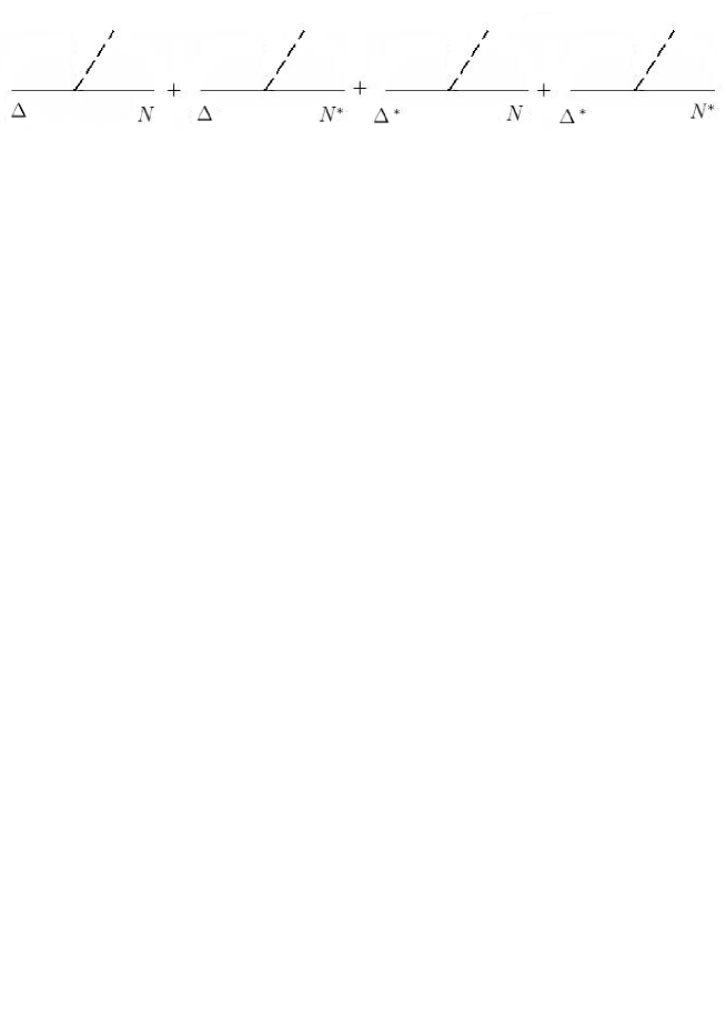
Figure 1: The four contributions to the spectral function in the presence of an external field: transition between ground state N to ground state $\Delta$, transitions between ground state N and excited states $\Delta^{*}$, transition between excited state $N^{*}$ and ground state $\Delta$ and pure excited states $N^{*}\to\Delta^{*}$.

Upon Borel transform, it takes the form

$$\begin{array}[]{l}\frac{C_{1}}{M^{2}}e^{-{\bar{m}}^{2}/M^{2}}+\sum\limits_{N^{*},\Delta^{*}}\frac{C_{4}}{M^{2}}e^{-\bar{m}^{*2}/{M^{2}}}\\ +e^{-\bar{m}^{2}/M^{2}}\left[e^{(\bar{m}^{2}-m_{\Delta}^{2})/M^{2}}\sum\limits_{N^{*}}{C_{2}(1-e^{-(m_{\Delta}^{2}-m_{N^{*}}^{2})/M^{2}})\over m_{\Delta}^{2}-m_{N^{*}}^{2}}+e^{(\bar{m}^{2}-m_{N}^{2})/M^{2}}\sum\limits_{\Delta^{*}}{C_{3}(1-e^{-(m_{\Delta^{*}}^{2}-m_{N}^{2})/M^{2}})\over m_{\Delta^{*}}^{2}-m_{N}^{2}}.\right]\end{array}$$ (34)

The important point is that the non-diagonal transitions ($N^{*}$ to $\Delta$ and $N$ to $\Delta^{*}$) give rise to a contribution that is not exponentially suppressed relative to the ground state. This is a general feature of the external-field technique. The strength of such transitions at each structure is a priori unknown and is a potential source of contamination in the determination of the amplitudes. The standard treatment of the off-digonal transitions is to approximate it (the quantity in the square brackets) by a parameter A, which is to be extracted from the sum rule along with the ground state property of interest. Inclusion of such contributions is necessary for the correct extraction of the amplitudes. The pure excited state transitions ($N^{*}$ to $\Delta^{*}$) are exponentially suppressed relative to the ground state and can be modeled in the usual way by introducing a continuum model and threshold parameter $w$.

In summary, we identified 12 different tensor structures from which 12 sum rules can be constructed, once the correlation function is evaluated at the quark level.

III.3 Calculation of the QCD side

We start by writing down the master formulas used in the calculation of the QCD side, which are functions of the quark propagators, obtained by contracting out pairs of time-ordered quark-field operators in the two-point correlation function in Eq. (15) using the interpolating fields in Eq. (18) and Eq. (19). We note that the same master formulas enter lattice QCD calculations where the fully-interacting quark propagators are generated numerically, instead of the analytical ones used here. The master formula for the transition $\gamma p\to\Delta^{+}$ (with $uud$ quark content) is:

$$\begin{array}[]{l}<0|T\{\eta_{\alpha}^{\Delta^{+}}(x)\bar{\eta}^{p}(0)\}|0>=-\frac{4}{{\sqrt{3}}}\varepsilon^{abc}\varepsilon^{a^{\prime}b^{\prime}c^{\prime}}\{\\ S_{u}^{aa^{\prime}}\gamma_{5}CS_{d}^{bb^{\prime T}}C\gamma_{\alpha}S_{u}^{cc^{\prime}}+S_{u}^{aa^{\prime}}Tr(\gamma_{5}CS_{u}^{Tbb^{\prime}}C\gamma_{\alpha}S_{d}^{cc^{\prime}})\\ -S_{d}^{aa^{\prime}}\gamma_{5}CS_{u}^{Tbb^{\prime}}C\gamma_{\alpha}S_{u}^{cc^{\prime}}+\beta[S_{u}^{aa^{\prime}}CS_{d}^{Tbb^{\prime}}C\gamma_{\alpha}S_{u}^{cc^{\prime}}\gamma_{5}\\ +S_{u}^{aa^{\prime}}\gamma_{5}Tr(CS_{u}^{Tbb^{\prime}}C\gamma_{\alpha}S_{d}^{cc^{\prime}})-S_{d}^{aa^{\prime}}CS_{u}^{Tbb^{\prime}}C\gamma_{\alpha}S_{u}^{cc^{\prime}}]\}.\end{array}$$ (35)

It is not necessary to list all the master formulas for the other transitions separately. Only three are distinct; others can be obtained by making appropriate substitutions in the above expression as specified below:

• for $n\gamma\to\Delta^{0}$ (with $ddu$ quark content), interchange d quark and u quark in $p\gamma\to\Delta^{+}$,

• for $\Sigma^{+}\gamma\to\Sigma^{*+}$ (with $uus$ quark content), replace d quark by s quark in $p\gamma\to\Delta^{+}$,

• for $\Sigma^{-}\gamma\to\Sigma^{*-}$ (with $dds$ quark content), replace u quark by d quark in $\Sigma^{+}\gamma\to\Sigma^{*+}$,

• for $\Xi^{0}\gamma\to\Xi^{*0}$ (with $ssu$ quark content), interchange u quark and s quark in $\Sigma^{+}\gamma\to\Sigma^{*+}$,

• for $\Xi^{-}\gamma\to\Xi^{*-}$ (with $ssd$ quark content), replace u quark by d quark in $\Xi^{0}\gamma\to\Xi^{*0}$.

Here the interchange of two quarks is achieved by simply switching the corresponding propagators.

The master formula for $\Sigma^{0}\gamma\to\Sigma^{*0}$ (with $uds$ quark content) is:

$$\begin{array}[]{l}<0|T\{\eta_{\alpha}^{\Sigma^{*0}}(x)\bar{\eta}^{\Sigma^{0}}(0)\}|0>=\frac{2}{{\sqrt{3}}}\varepsilon^{abc}\varepsilon^{a^{\prime}b^{\prime}c^{\prime}}\{\\ S_{s}^{aa^{\prime}}\gamma_{5}CS_{u}^{Tbb^{\prime}}C\gamma_{\alpha}S_{d}^{cc^{\prime}}-S_{u}^{aa}\gamma_{5}CS_{s}^{Tbb^{\prime}}C\gamma_{\alpha}S_{d}^{cc^{\prime}}\\ -S_{d}^{aa^{\prime}}Tr(\gamma_{5}CS_{s}^{Tbb^{\prime}}C\gamma_{\alpha}S_{u}^{cc^{\prime}})+S_{s}^{aa^{\prime}}\gamma_{5}CS_{d}^{Tbb^{\prime}}C\gamma_{\alpha}S_{u}^{cc^{\prime}}\\ -S_{d}^{aa}\gamma_{5}CS_{s}^{Tbb^{\prime}}C\gamma_{\alpha}S_{u}^{cc^{\prime}}-S_{u}^{aa^{\prime}}Tr(\gamma_{5}CS_{s}^{Tbb^{\prime}}C\gamma_{\alpha}S_{d}^{cc^{\prime}})\\ +\beta[S_{s}^{aa^{\prime}}CS_{u}^{Tbb^{\prime}}C\gamma_{\alpha}S_{d}^{cc^{\prime}}\gamma_{5}-S_{u}^{aa^{\prime}}CS_{s}^{Tbb^{\prime}}C\gamma_{\alpha}S_{d}^{cc^{\prime}}\gamma_{5}\\ -S_{d}^{aa^{\prime}}\gamma_{5}Tr(CS_{s}^{Tbb^{\prime}}C\gamma_{\alpha}S_{u}^{cc^{\prime}})+S_{s}^{aa^{\prime}}CS_{d}^{Tbb^{\prime}}C\gamma_{\alpha}S_{u}^{cc^{\prime}}\gamma_{5}\\ -S_{d}^{aa^{\prime}}CS_{s}^{Tbb^{\prime}}C\gamma_{\alpha}S_{u}^{cc^{\prime}}\gamma_{5}-S_{u}^{aa^{\prime}}\gamma_{5}Tr(CS_{s}^{Tbb^{\prime}}C\gamma_{\alpha}S_{d}^{cc^{\prime}})].\end{array}$$ (36)

The master formula for $\Lambda\gamma\to\Sigma^{*0}$ (with $uds$ quark content) is:

$$\begin{array}[]{l}<0|T\{\eta_{\alpha}^{\Sigma^{*0}}(x)\bar{\eta}^{\Lambda}\}|0>=\frac{2}{3}\varepsilon^{abc}\varepsilon^{a^{\prime}b^{\prime}c^{\prime}}\{\\ 2S_{d}^{aa^{\prime}}\gamma_{5}CS_{u}^{Tbb^{\prime}}C\gamma_{\alpha}S_{s}^{cc^{\prime}}-2S_{u}^{aa}\gamma_{5}CS_{d}^{Tbb^{\prime}}C\gamma_{\alpha}S_{s}^{cc^{\prime}}\\ -2S_{s}^{aa^{\prime}}Tr(\gamma_{5}CS_{u}^{Tbb^{\prime}}C\gamma_{\alpha}S_{d}^{cc^{\prime}})+S_{s}^{aa^{\prime}}\gamma_{5}CS_{u}^{Tbb^{\prime}}C\gamma_{\alpha}S_{d}^{cc^{\prime}}\\ -S_{u}^{aa}\gamma_{5}CS_{s}^{Tbb^{\prime}}C\gamma_{\alpha}S_{d}^{cc^{\prime}}-S_{d}^{aa^{\prime}}Tr(\gamma_{5}CS_{s}^{Tbb^{\prime}}C\gamma_{\alpha}S_{u}^{cc^{\prime}})\\ -S_{s}^{aa^{\prime}}\gamma_{5}CS_{d}^{Tbb^{\prime}}C\gamma_{\alpha}S_{u}^{cc^{\prime}}+S_{d}^{aa}\gamma_{5}CS_{s}^{Tbb^{\prime}}C\gamma_{\alpha}S_{u}^{cc^{\prime}}\\ +S_{u}^{aa^{\prime}}Tr(\gamma_{5}CS_{s}^{Tbb^{\prime}}C\gamma_{\alpha}S_{d}^{cc^{\prime}})+\beta[-2S_{d}^{aa^{\prime}}CS_{u}^{Tbb^{\prime}}C\gamma_{\alpha}S_{s}^{cc^{\prime}}\gamma_{5}\\ +2S_{u}^{aa}CS_{d}^{Tbb^{\prime}}C\gamma_{\alpha}S_{s}^{cc^{\prime}}\gamma_{5}-2S_{s}^{aa^{\prime}}Tr(CS_{u}^{Tbb^{\prime}}C\gamma_{\alpha}S_{d}^{cc^{\prime}})\gamma_{5}\\ +S_{s}^{aa^{\prime}}CS_{u}^{Tbb^{\prime}}C\gamma_{\alpha}S_{d}^{cc^{\prime}}\gamma_{5}-S_{u}^{aa}CS_{s}^{Tbb^{\prime}}C\gamma_{\alpha}S_{d}^{cc^{\prime}}\gamma_{5}\\ -S_{d}^{aa^{\prime}}Tr(CS_{s}^{Tbb^{\prime}}C\gamma_{\alpha}S_{u}^{cc^{\prime}})\gamma_{5}-S_{s}^{aa^{\prime}}CS_{d}^{Tbb^{\prime}}C\gamma_{\alpha}S_{u}^{cc^{\prime}}\gamma_{5}\\ +S_{d}^{aa}CS_{s}^{Tbb^{\prime}}C\gamma_{\alpha}S_{u}^{cc^{\prime}}\gamma_{5}+S_{u}^{aa^{\prime}}Tr(CS_{s}^{Tbb^{\prime}}C\gamma_{\alpha}S_{d}^{cc^{\prime}})\gamma_{5}]\}.\end{array}$$ (37)

In the above equations,

$$S^{ab}_{q}(x,0;F)\equiv\langle 0\,|\,T\{\;q^{a}(x)\,\bar{q}^{b}(0)\;\}\,|\,0\rangle_{F},\hskip 8.53581ptq=u,d,s,$$ (38)

is the fully interacting quark propagator in the presence of the electromagnetic field. It is obtained by the operator product expansion (OPE) and is made of dozens of analytic terms. It has been discussed to various degree in the literature Ioffe84 ; Pasupathy86 ; Wilson87 ; Wang08 so we will not list the terms here.

In addition to the standard vacuum condensates, the vacuum susceptibilities induced by the external field are defined by

$$\begin{array}[]{rcl}\langle\bar{q}\sigma_{\mu\nu}q\rangle_{F}&\equiv&e_{q}\chi\langle\bar{q}q\rangle F_{\mu\nu},\\ \langle\bar{q}g_{c}G_{\mu\nu}q\rangle_{F}&\equiv&e_{q}\kappa\langle\bar{q}q\rangle F_{\mu\nu},\\ \langle\bar{q}g_{c}\epsilon_{\mu\nu\rho\lambda}G^{\rho\lambda}\gamma_{5}q\rangle_{F}&\equiv&ie_{q}\xi\langle\bar{q}q\rangle F_{\mu\nu}.\end{array}$$ (39)

Note that $\chi$ has the dimension of GeV^-2, while $\kappa$ and $\xi$ are dimensionless.

Figure 2: Diagrams considered for the calculation of N to $\Delta$ transitions that do not contain strange quark mass terms.

Figure 3: Diagrams considered for the calculation of N to $\Delta$ transitions that are proportional to the strange quark mass (denoted by $\times$).

With the above elements in hand, it is straightforward to evaluate the correlation function by substituting the quark propagator into the various master formulas. We keep terms to first order in the external field and in the strange quark mass (u-quark and d-quark masses are ignored). Vacuum condensates up to dimension eight are retained in the expansion. The algebra is extremely tedious. Each term in the master formula is a product of three copies of the quark propagator, and there are hundreds of such terms over various color permutations. The calculation can be organized by the diagrams (similar to Feynmann diagrams) in Fig. 2 and Fig. 3. Note that each diagram is only generic and all possible color permutations are implied. We used the computer algebra package called REDUCE to carry out some of the calculations. The QCD side has the same tensor structure as the phenomenological side and the results can be collected according to the same 12 independent tensor structures in Eq. (29).

III.4 The QCD sum rules

Once we have both the QCD side (commonly referred as LHS) and the phenomenological side (RHS), we can isolate the sum rules by matching the two sides. Since there are 12 independent tensor structures, 12 sum rules can be constructed for each transition. For the 8 transitions, the total number of sum rules is 96. We divide the sum rules into four groups according to their dependence on the amplitudes and performance. The first group consists of the sum rules at structures $\mbox{WE}_{1}$, $\mbox{WO}_{2}$ and $\mbox{WE}_{3}$ which only contain the amplitude $G_{1}$, and at $\mbox{WE}_{6}$ which only contains $G_{2}$. These sum rules are expected to perform better because they involve fewer parameters. The second group consists of the sum rules at structures $\mbox{WE}_{5}$, $\mbox{WO}_{5}$ and $\mbox{WO}_{6}$ which have both $G_{1}$ and $G_{2}$. It is difficult to extract both amplitudes at the same time. One way out is to fix one of them and treat the other as free parameter. This reduces the predictive ability of the QCD sum rules. Our numerical analysis suggests that it can serve as a consistence check at best. Another way is to take appropriate combinations of sum rules to eliminate one of the amplitudes. We tried but found the sum rules obtained this way perform worse than the un-manipulated ones. We advocate against the practice of manipulating the original sum rules like algebraic equations (such as taking derivatives or linear combinations) to obtain new sum rules. The third group consists of the sum rules at structures $\mbox{WE}_{2}$, $\mbox{WO}_{1}$ and $\mbox{WO}_{3}$ which have one of the amplitudes and additional dependence on the averaged square mass $\bar{m}^{2}$, aside from the common factor $e^{-\bar{m}^{2}/M^{2}}$. We found these sum rules perform consistently worse than those in groups 1 and 2, possibly because of the approximation introduced by $\bar{m}^{2}$. The fourth group consists of the sum rules at $\mbox{WE}_{4}$ and $\mbox{WO}_{4}$ which contain both $G_{1}$ and $G_{2}$, and additional $\bar{m}^{2}$ dependence. They perform consistently the worst. In the following, we are going to give detailed analysis of the sum rules in group 1, but first let us present the sum rules in this group.

At the structure $\mbox{WE}_{1}$, the sum rules can be expressed in the following form:

$$\begin{array}[]{l}c_{1}L^{-4/27}E_{2}(w)M^{4}+c_{2}\chi am_{s}L^{-20/27}E_{1}(w)M^{2}\\ +c_{3}am_{s}L^{-4/27}E_{0}(w)+c_{4}\chi a^{2}L^{4/27}E_{0}(w)\\ +c_{5}bL^{-4/27}E_{0}(w)+c_{6}m_{0}^{2}am_{s}L^{-18/27}\frac{1}{M^{2}}\\ +c_{7}a^{2}L^{20/27}\frac{1}{M^{2}}+c_{8}\chi m_{0}^{2}a^{2}L^{-10/27}\frac{1}{M^{2}}\\ =\tilde{\lambda}_{N}\tilde{\lambda}_{\Delta}e^{-\bar{m}^{2}/M^{2}}[\frac{{1}}{3M^{2}}G_{1}(m_{\Delta}+m_{N})+A].\end{array}$$ (40)

Here $\tilde{\lambda}_{N}$ and $\tilde{\lambda}_{\Delta}$ are the rescaled current coupling ${\tilde{\lambda}^{2}\equiv(2\pi)^{4}\lambda^{2}}$. The quark condensate, gluon condensate, and the mixed condensate are represented by

$$a=-(2\pi)^{2}\,\langle\bar{u}u\rangle,\hskip 5.69054ptb=\langle g^{2}_{c}\,G^{2}\rangle,\hskip 5.69054ptm_{0}^{2}=-\langle\bar{u}g_{c}\sigma\cdot Gu\rangle/\langle\bar{u}u\rangle.$$ (41)

The quark charge factors $e_{q}$ are given in units of electric charge

$$e_{u}=2/3,\hskip 11.38109pte_{d}=-1/3,\hskip 11.38109pte_{s}=-1/3.$$ (42)

Note that we choose to keep the quark charge factors explicit in the sum rules. The advantage is that it can facilitate the study of individual quark contributions to the amplitudes. The parameters $f$ and $\phi$ account for the flavor-symmetry breaking of the strange quark in the condensates and susceptibilities:

$$f={\langle\bar{s}s\rangle\over\langle\bar{u}u\rangle}={\langle\bar{s}g_{c}\sigma\cdot Gs\rangle\over\langle\bar{u}g_{c}\sigma\cdot Gu\rangle},\hskip 11.38109pt\phi={\chi_{s}\over\chi}={\kappa_{s}\over\kappa}={\xi_{s}\over\xi}.$$ (43)

The anomalous dimension corrections of the interpolating fields and the various operators are taken into account in the leading logarithmic approximation via the factor

$$L^{\gamma}=[{\alpha_{s}(\mu^{2})\over\alpha_{s}(M^{2})}]^{\gamma}=[{\ln(M^{2}/\Lambda_{QCD}^{2})\over\ln(\mu^{2}/\Lambda_{QCD}^{2})}]^{\gamma},$$ (44)

where $\mu=500$ MeV is the renormalization scale and $\Lambda_{QCD}$ is the QCD scale parameter. As usual, the pure excited state contributions are modeled using terms on the OPE side surviving $M^{2}\rightarrow\infty$ under the assumption of duality, and are represented by the factors

$$E_{n}(w)=1-e^{-w^{2}/M^{2}}\sum_{n}{(w^{2}/M^{2})^{n}\over n!},$$ (45)

where $w$ is an effective continuum threshold and it is in principle different for different sum rules and we will treat it as a free parameter in the analysis.

The $c_{i}$ coefficients differ from transition to transition. It is not necessary to list the coefficients separately for all 8 transition channels. We only need to carry out three separate calculations for $\Sigma^{+}\gamma\to\Sigma^{*+}$, $\Xi^{0}\gamma\to\Xi^{*0}$ and $\Lambda\gamma\to\Sigma^{*0}$. Other channels can be obtained from them by making appropriate substitutions as specified below:

• for $p\gamma\to\Delta^{+}$, replace s quark by d quark in $\Sigma^{+}\gamma\to\Sigma^{*+}$,

• for $n\gamma\to\Delta^{0}$, interchange d quark and u quark in proton $p\gamma\to\Delta^{+}$,

• for $\Sigma^{-}\gamma\to\Sigma^{*-}$, replace u quark by d quark in $\Sigma^{+}\gamma\to\Sigma^{*+}$,

• for $\Sigma^{0}\gamma\to\Sigma^{*0}$, add corresponding coefficients of $\Sigma^{+}\gamma\to\Sigma^{*+}$ and $\Sigma^{-}\gamma\to\Sigma^{*-}$, then divide by 2,

• for $\Xi^{-}\gamma\to\Xi^{*0}$, replace u quark by d quark in $\Xi^{0}\gamma\to\Xi^{*0}$.

Here the interchange between u and d quarks is achieved by simply switching their charge factors $e_{u}$ and $e_{d}$. The conversions from s quark to u or d quarks involve setting $m_{s}=0$, $f=\phi=1$, in addition to switching the charge factors. In practice, we computed all 8 channels separately, and used the substitutions as a check of our calculations.

The coefficients appearing in Eq.( 40) are given by, in the transition channel $\Sigma^{+}\gamma\to\Sigma^{*+}$,

$$\begin{array}[]{l}c_{1}=\frac{1}{4}(-1+\beta)(e_{s}-e_{u}),\\ c_{2}=-\frac{1}{4}(1+2\beta)(e_{u}-e_{s}f_{s}\phi),\\ c_{3}=\frac{1}{12}(e_{u}(-1+\beta+3f_{s}+3\beta f_{s}+\kappa-\beta\kappa-(2+\beta)\xi)\\ \;\;\;+e_{s}(-6+f_{s}(4-\kappa\phi+2\phi\xi)+\beta(-6+f_{s}(2+\phi(\kappa+\xi))))),\\ c_{4}=\frac{1}{6}(-e_{u}(1+\beta+f_{s})+(2+\beta)e_{s}f_{s}\phi),\\ c_{5}=-\frac{1}{48}(-1+\beta)(e_{s}-e_{u}),\\ c_{6}=\frac{1}{24}(1+2\beta)(2e_{s}-e_{u}(1+f_{s})),\\ c_{7}=\frac{1}{36}(-e_{u}(2-5\kappa+\xi+\beta(2+\kappa+\xi)+f_{s}(-4+4\kappa+\xi))\\ \;\;\;+e_{s}(-6+f_{s}(4+2\beta-\kappa\phi+\beta\kappa\phi+(2+\beta)\phi\xi))),\\ c_{8}=\frac{1}{144}(e_{u}(8+2\beta+8f_{s}+5\beta f_{s})-(16+7\beta)e_{s}f_{s}\phi);\end{array}$$ (46)

in the transition channel $\Xi^{0}\gamma\to\Xi^{*0}$,

$$\begin{array}[]{l}c_{1}=-\frac{1}{8}(-1+\beta)(e_{s}-e_{u}),\\ c_{2}=\frac{1}{8}(1+3\beta)(e_{u}-e_{s}f_{s}\phi),\\ c_{3}=\frac{1}{12}(e_{s}f_{s}-e_{s}f_{s}\phi(\kappa+\xi)+e_{u}(2-3f_{s}+\kappa+\xi)\\ \;\;\;+\beta(e_{u}(8-3f_{s}+\kappa+\xi)-e_{s}(6+f_{s}(-1+\phi(\kappa+\xi))))),\\ c_{4}=\frac{1}{6}(1+\beta)f_{s}(e_{u}-e_{s}f_{s}\phi),\\ c_{5}=\frac{1}{192}(-1+\beta)(e_{s}-e_{u}),\\ c_{6}=\frac{1}{48}(e_{s}(2-\beta(-4+f_{s})-5f_{s})\\ \;\;\;+e_{u}(1+2f_{s}+\beta(-7+4f_{s}))),\\ c_{7}=\frac{1}{36}(e_{u}(-3(1+\beta)f_{s}^{2}+3(1+\beta)\kappa\\ \;\;\;+f_{s}(2-2\kappa+\xi+\beta(8-2\kappa+\xi)))\\ \;\;\;+e_{s}(-3+f_{s}(6-3\kappa\phi+f_{s}(-2+2\kappa\phi-\phi\xi))\\ \;\;\;+\beta(-3-3f_{s}\kappa\phi+f_{s}^{2}(-2+2\kappa\phi-\phi\xi)))),\\ c_{8}=-\frac{1}{144}(1+\beta)(e_{u}(-1+8f_{s})-e_{s}f_{s}(2+5f_{s})\phi);\end{array}$$ (47)

and in the transition channel $\Lambda\gamma\to\Sigma^{*0}$,

$$\begin{array}[]{l}c1=\frac{1}{8}(-(2+\beta)e_{d}+e_{s}+(2+\beta)e_{u}),\\ c_{2}=\frac{1}{8}((3-2\beta)e_{d}+2(-1+\beta)e_{u}),\\ c_{3}=\frac{1}{24}(e_{d}(-2-12f_{s}-\kappa+\beta(1+3f_{s}-\kappa-\xi)+5\xi)\\ \;\;\;+e_{u}(-2+6f_{s}+5\kappa-4\xi+\beta(-1-3f_{s}+\kappa+\xi))\\ \;\;\;+e_{s}(-6+f_{s}(-2+2\kappa\phi-\phi\xi))),\\ c_{4}=\frac{1}{12}(-e_{u}(2-3\beta+2(1+\beta)f_{s})\\ \;\;\;+e_{d}(3+2f_{s}+\beta(-3+2f_{s}))-e_{s}f_{s}\phi),\\ c_{5}=\frac{1}{192}((5+2\beta)e_{d}+3e_{s}-(3+2\beta)e_{u}),\\ c_{6}=\frac{1}{96}(-2e_{s}-(-9+4\beta)e_{d}(1+f_{s})+(-5+4\beta)e_{u}(1+f_{s})),\\ c_{7}=\frac{1}{72}(e_{s}f_{s}(-2+2\kappa\phi-\phi\xi)+e_{d}(2f_{s}(-7-2\kappa+\xi)\\ \;\;\;+3(2+\kappa+\xi)+\beta(-3+2f_{s})(2+\kappa+\xi))-e_{u}(2(2+\kappa+\xi)\\ \;\;\;+\beta(-3+2f_{s})(2+\kappa+\xi)+f_{s}(-8-7\kappa+2\xi))),\\ c_{8}=\frac{1}{288}(-e_{d}(23+17f_{s}+\beta(-20+13f_{s}))\\ \;\;\;+e_{u}(15(1+f_{s})+\beta(-20+13f_{s}))).\end{array}$$ (48)

At structure $\mbox{WE}_{6}$, the sum rule is:

$$\begin{array}[]{l}c_{1}\chi am_{s}L^{-20/27}E_{1}(w)M^{2}+c_{2}am_{s}L^{-4/27}E_{0}(w)\\ +c_{3}\chi a^{2}L^{4/27}E_{0}(w)+c_{4}a^{2}L^{20/27}\frac{1}{M^{2}}+c_{5}\chi m_{0}^{2}a^{2}L^{-10/27}\frac{1}{M^{2}}\\ =\tilde{\lambda}_{N}\tilde{\lambda}_{\Delta}e^{-\bar{m}^{2}/M^{2}}[\frac{{1}}{M^{2}}G_{2}(m_{N}^{2}-m_{\Delta}m_{N})+A].\end{array}$$ (49)

The coefficients appearing in Eq.( 49) are given by, in the transition channel $\Sigma^{+}\gamma\to\Sigma^{*+}$,

$$\begin{array}[]{l}c_{1}=\beta(-e_{u}+e_{s}f_{s}\phi),\\ c_{2}=\frac{1}{3}\beta(e_{u}(-4-2\kappa+\xi)+e_{s}f_{s}(4+2\kappa\phi-\phi\xi)),\\ c_{3}=-\frac{2}{3}\beta(e_{u}-e_{s}f_{s}\phi),\\ c_{4}=\frac{1}{18}(-3e_{u}(-1+f_{s})\xi+2\beta(e_{u}(-4-2\kappa+\xi)\\ \;\;\;+e_{s}f_{s}(4+2\kappa\phi-\phi\xi))),\\ c_{5}=\frac{1}{6}\beta(e_{u}-e_{s}f_{s}\phi);\end{array}$$ (50)

in the transition channel $\Xi^{0}\gamma\to\Xi^{*0}$,

$$\begin{array}[]{l}c_{1}=\beta(e_{u}-e_{s}f_{s}\phi),\\ c_{2}=\frac{1}{3}\beta(e_{u}(4+2\kappa-\xi)+e_{s}f_{s}(-4-2\kappa\phi+\phi\xi)),\\ c_{3}=\frac{2}{3}\beta f_{s}(e_{u}-e_{s}f_{s}\phi),\\ c_{4}=\frac{1}{18}f_{s}(3e_{s}(-1+f_{s})\phi\xi+2\beta(e_{u}(4+2\kappa-\xi)\\ \;\;\;+e_{s}f_{s}(-4-2\kappa\phi+\phi\xi))),\\ c_{5}=\frac{1}{6}\beta f_{s}(-e_{u}+e_{s}f_{s}\phi);\end{array}$$ (51)

and in the transition channel $\Lambda\gamma\to\Sigma^{*0}$,

$$\begin{array}[]{l}c_{1}=\frac{1}{2}\beta(e_{d}-e_{u}),\\ c_{2}=\frac{1}{6}\beta(e_{d}-e_{u})(4+2\kappa-\xi),\\ c_{3}=\frac{1}{3}\beta(e_{d}-e_{u}),\\ c_{4}=\frac{1}{36}(e_{d}-e_{u})(\beta(8+4\kappa-2\xi)-3(-1+f_{s})\xi),\\ c_{5}=\frac{1}{12}\beta(-e_{d}+e_{u}).\end{array}$$ (52)

At structure $\mbox{WO}_{2}$, the sum rule is:

$$\begin{array}[]{l}c_{1}m_{s}L^{-16/27}E_{1}(w)M^{2}+c_{2}\chi aL^{-8/27}E_{1}(w)M^{2}\\ +c_{3}aL^{8/27}E_{0}(w)+c_{4}m_{0}^{2}aL^{-6/27}\frac{1}{M^{2}}+c_{5}\chi a^{2}m_{s}L^{-8/27}\frac{1}{M^{2}}\\ +c_{6}\chi abL^{-8/27}\frac{1}{M^{2}}+c_{7}a^{2}m_{s}L^{8/27}\frac{1}{M^{4}}+c_{8}abL^{8/27}\frac{1}{M^{4}}\\ =\tilde{\lambda}_{N}\tilde{\lambda}_{\Delta}e^{-\bar{m}^{2}/M^{2}}[\frac{{1}}{3M^{2}}G_{1}\frac{1}{m_{\Delta}}(m_{N}+m_{\Delta})+A].\end{array}$$ (53)

The coefficients appearing in Eq.( 53) are given by, in the transition channel $\Sigma^{+}\gamma\to\Sigma^{*+}$,

$$\begin{array}[]{l}c_{1}=\frac{1}{2}(-e_{s}+e_{u}),\\ c_{2}=\frac{1}{6}(-e_{u}+e_{s}f_{s}\phi),\\ c_{3}=\frac{1}{12}(e_{u}(-2+6f_{s}+2\kappa+6\beta(-2+2f_{s}+\kappa)-\xi)\\ \;\;\;+e_{s}(-6+f_{s}(2-2(1+3\beta)\kappa\phi+\phi\xi))),\\ c_{4}=\frac{1}{12}(4e_{s}-e_{u}(1+2\beta(-1+f_{s})+3f_{s})),\\ c_{5}=\frac{1}{6}(e_{u}(1+4\beta(-1+f_{s})+3f_{s})-4e_{s}f_{s}\phi),\\ c_{6}=\frac{1}{72}\beta(e_{u}-e_{s}f_{s}\phi),\\ c_{7}=\frac{1}{36}(e_{s}(6+f_{s}(-4+\phi(\kappa+6\beta\kappa-2\xi)))\\ \;\;\;+e_{u}(2-2\kappa+\xi+f_{s}(-4+\kappa-6\beta\kappa+\xi))),\\ c_{8}=\frac{1}{144}(-2e_{s}+e_{u}(1-2\beta(-1+f_{s})+f_{s}));\end{array}$$ (54)

in the transition channel $\Xi^{0}\gamma\to\Xi^{*0}$,

$$\begin{array}[]{l}c_{1}=\frac{1}{4}(1+\beta)(e_{s}-e_{u}),\\ c_{2}=-\frac{1}{12}(-1+\beta)(e_{u}-e_{s}f_{s}\phi),\\ c_{3}=\frac{1}{24}(e_{u}(2-6f_{s}+\kappa+\xi)-e_{s}f_{s}(-4+\phi(\kappa+\xi))\\ \;\;\;+\beta(e_{u}(-14+6f_{s}-7\kappa-\xi)\\ \;\;\;+e_{s}(24+f_{s}(-16+7\kappa\phi+\phi\xi)))),\\ c_{4}=\frac{1}{48}(-2(e_{s}+6\beta e_{s}+e_{u}-6\beta e_{u})\\ \;\;\;+((-5+7\beta)e_{s}+(9-7\beta)e_{u})f_{s}),\\ c_{5}=\frac{1}{12}(\beta(-1+f_{s})(2e_{u}-7e_{s}f_{s}\phi)\\ \;\;\;+f_{s}(-4e_{u}+e_{s}(1+3f_{s})\phi)),\\ c_{6}=-\frac{1}{288}(-1+3\beta)(e_{u}-e_{s}f_{s}\phi),\\ c_{7}=\frac{1}{72}(e_{s}(12+2f_{s}(-8-5\beta+f_{s}+(2+\beta(-5+f_{s})-f_{s})\\ \;\;\;\kappa\phi)-(-1+\beta)f_{s}(1+f_{s})\phi\xi)+2e_{u}(-3\kappa+f_{s}(-2+3f_{s}\\ \;\;\;+2\kappa-\xi)+\beta(2+\kappa+3f_{s}(1+\kappa)+\xi))),\\ c_{8}=\frac{1}{576}(-2(-1+2\beta)(e_{s}+e_{u})\\ \;\;\;+(e_{s}+5\beta e_{s}+(-5+3\beta)e_{u})f_{s});\end{array}$$ (55)

and in the transition channel $\Lambda\gamma\to\Sigma^{*0}$,

$$\begin{array}[]{l}c1=\frac{1}{4}(-3e_{d}+e_{s}+2e_{u}),\\ c_{2}=\frac{1}{6}({e_{d}-e_{u}}),\\ c_{3}=\frac{1}{24}(6e_{s}+e_{u}(2+6f_{s}+7\kappa-6\beta(-2+2f_{s}+\kappa)-2\xi)\\ \;\;\;+e_{d}(-8-6f_{s}-7\kappa+6\beta(-2+2f_{s}+\kappa)+2\xi)),\\ c_{4}=\frac{1}{96}(e_{d}(30+\beta(23-22f_{s})+16f_{s})\\ \;\;\;+e_{u}(-2(7+8f_{s})+\beta(-23+26f_{s}))),\\ c_{5}=\frac{1}{6}(e_{d}(-3+2\beta(-1+f_{s})-2f_{s})\\ \;\;\;+2e_{u}(1+\beta+f_{s}-\beta f_{s})+e_{s}f_{s}\phi),\\ c_{6}=\frac{1}{288}((-1+2\beta)e_{d}-(1+2\beta)e_{u}),\\ c_{7}=\frac{1}{72}(-6e_{s}-e_{u}(\kappa-12\beta\kappa\\ \;\;\;+f_{s}(8+(4+6\beta)\kappa-2\xi)-2(2+\xi))\\ \;\;\;+e_{d}(f_{s}(14+\kappa+6\beta\kappa-2\xi)-2(2+(-2+6\beta)\kappa+\xi))),\\ c_{8}=\frac{1}{1152}(1-8e_{s}+e_{u}(6+\beta(7-10f_{s})+8f_{s})\\ \;\;\;+e_{d}(-14-7\beta-8f_{s}+6\beta f_{s})).\end{array}$$ (56)

This concludes the presentation of the QCD sum rules that will be used in the numerical analysis.

IV Sum Rule Analysis

IV.1 General procedure

The sum rules for N to $\Delta$ transition have the generic form of OPE - ESC = Pole + Transition, or

$$\begin{array}[]{l}\Pi_{tran}(QCD,\beta,w,M^{2})=\\ \;\;\;\;\;\;\;\;\;\;\tilde{\lambda}_{N}\tilde{\lambda}_{\Delta}\left({f(G_{1},G_{2})\over M^{2}}+A\right)e^{-\bar{m}^{2}/M^{2}},\end{array}$$ (57)

where $QCD$ represents all the QCD input parameters. $f(G_{1},G_{2})$ is a function of transition amplitudes $G_{1}$ and $G_{2}$. The basic mathematical task is: given the function $\Pi_{tran}$ with known QCD input parameters, find the phenomenological parameters ($G_{1}$, $G_{2}$, transition strength $A$, coupling strength $\tilde{\lambda}$, and continuum threshold $w$) by matching the two sides over some region in the Borel mass $M$. A $\chi^{2}$ minimization is best suited for this purpose. It turns out that there are too many fit parameters for this procedure to be successful in general. To alleviate the situation, we employ the corresponding mass sum rules which have a generic form of OPE - ESC = Pole, or

$$\Pi_{mass,N}(QCD,\beta,w_{1},M^{2})=\tilde{\lambda}_{N}^{2}e^{-m_{N}^{2}/M^{2}};$$ (58)

$$\Pi_{mass,\Delta}(QCD,\beta,w_{2},M^{2})=\tilde{\lambda}_{\Delta}^{2}e^{-m_{\Delta}^{2}/M^{2}}.$$ (59)

They share some of the common parameters and factors with the transition sum rules. Note that the continuum thresholds may not be the same in different sum rules. By taking the following combination of the transition and mass sum rules,

$$\begin{array}[]{l}\frac{\Pi_{tran}(QCD,\beta,w,M^{2})}{\sqrt{\Pi_{mass,N}(QCD,\beta,w_{1},M^{2})\Pi_{mass,\Delta}(QCD,\beta,w_{2},M^{2})}}\\ =\frac{f(G_{1},G_{2})}{M^{2}}+A,\end{array}$$ (60)

the couplings $\lambda$ and the exponential factors are canceled out. This is another advantage for introducing the $\bar{m}^{2}$ prescription. The form in Eq. (60) is what we are going to implement. By plotting the two sides as a function of $1/M^{2}$, the slope will be related to the transition amplitudes $G_{1}$ or $G_{2}$ and the intercept the transition strength A. The linearity (or deviation from it) of the left-hand side gives an indication of OPE convergence and the role of excited states. The two sides are expected to match for a good sum rule over a certain window. This way of matching the sum rules has two advantages. First, the slope, which is proportional to the transition amplitudes, is usually better determined than the intercept. Second, by allowing the possibility of different continuum thresholds, we ensure that both sum rules stay in their valid regimes.

For the octet baryons, we use the chiral-even mass sum rules in Ref. Lee02 which are reproduced here in the same notation used in this work.

$$\begin{array}[]{l}p_{1}L^{-4/9}E_{3}(w_{1})M^{6}+p_{2}bL^{-4/9}E_{1}(w_{1})M^{2}+p_{3}m_{s}aL^{4/9}\\ +p_{4}a^{2}L^{4/9}+p_{5}a^{2}k_{v}L^{4/9}+p_{6}m_{0}^{2}a^{2}L^{-2/27}\frac{1}{M^{2}}\\ =\tilde{\lambda}_{N}^{2}e^{-m_{N}^{2}/M^{2}}.\end{array}$$ (61)

The coefficients are, for N:

$$\begin{array}[]{*{20}l}\begin{array}[]{l}p_{1}=\frac{1}{64}(5+2\beta+5\beta^{2}),\;\;\;p_{2}=\frac{1}{256}(5+2\beta+5\beta^{2}),\\ p_{3}=0,p_{4}=\frac{1}{24}(7-2\beta-5\beta),\;\;\;p_{5}=0,\\ p_{6}=-\frac{1}{96}(13-2\beta-11\beta^{2});\end{array}\end{array}$$ (62)

for $\Lambda$:

$$\begin{array}[]{*{20}l}\begin{array}[]{l}p_{1}=\frac{1}{64}(5+2\beta+5\beta^{2}),\\ p_{2}=\frac{1}{256}(5+2\beta+5\beta^{2}),\\ p_{3}=\frac{1}{96}((20-15f_{s})-(16+6f_{s})\beta-(4+15f_{s})\beta^{2}),\\ p_{4}=\frac{1}{96}((4f_{s}-5-6t)+(4+4f_{s})\beta+(4f_{s}+1+6t)\beta^{2}),\\ p_{5}=\frac{1}{72}((10f_{s}+11)+(2-8f_{s})\beta-(2f_{s}+13)\beta^{2}),\\ p_{6}=\frac{1}{288}((-16f_{s}-23)+(8f_{s}-2)\beta+(8f_{s}+25)\beta^{2});\end{array}\end{array}$$ (63)

for $\Sigma$:

$$\begin{array}[]{*{20}l}\begin{array}[]{l}p_{1}=\frac{1}{64}(5+2\beta+5\beta^{2}),\\ p_{2}=\frac{1}{256}(5+2\beta+5\beta^{2}),\\ p_{3}=\frac{1}{32}((12-5f_{s})-2f_{s}\beta-(12+5f_{s})\beta^{2}),\\ p_{4}=-\frac{1}{94}((4f_{s}+21+18t)+4f_{s}\beta+(4f_{s}-21-18t)\beta^{2}),\\ p_{5}=\frac{1}{24}((6f_{s}+1)-2\beta-(6f_{s}-1)\beta^{2}),\\ p_{6}=-\frac{1}{96}((12f_{s}+1)-2\beta-(12f_{s}-1)\beta^{2});\end{array}\end{array}$$ (64)

for $\Xi$:

$$\begin{array}[]{*{20}l}\begin{array}[]{l}p_{1}=\frac{1}{64}(5+2\beta+5\beta^{2}),\\ p_{2}=\frac{1}{256}(5+2\beta+5\beta^{2}),\\ p_{3}=\frac{3}{16}((2-f_{s})-2f_{s}\beta-(2+f_{s})\beta^{2}),\\ p_{4}=-\frac{1}{96}((15-f_{s}+18t)-10f_{s}\beta-(15+f_{s}+18t)\beta^{2}),\\ p_{5}=\frac{1}{24}f_{s}((f_{s}+6)-2f_{s}\beta+(f_{s}-6)\beta^{2}),\\ p_{6}=-\frac{1}{94}f_{s}((f_{s}+12)-2f_{s}\beta+(f_{s}-12)\beta^{2}).\end{array}\end{array}$$ (65)

The function t is defined as $t\equiv\ln{\frac{M^{2}}{\mu^{2}}}-\gamma_{EM}$ with $\gamma_{EM}\approx 0.577$ the Euler-Mascheroni constant.

For the decuplet baryons, we use the chiral-odd sum rules Lee98 at the structure $g_{\scriptscriptstyle\mu\nu}$, which are reproduced here, for $\Delta$:

$$\begin{array}[]{l}{4\over 3}\,a\;E_{1}\,L^{16/27}\;M^{4}-{2\over 3}\,m^{2}_{0}a\;E_{0}\,L^{2/27}\;M^{2}-{1\over 18}\,a\,b\;L^{16/27}\\ =\tilde{\lambda}_{\scriptscriptstyle\Delta}^{2}\;M_{\scriptscriptstyle\Delta}\;e^{-M_{\scriptscriptstyle\Delta}^{2}/M^{2}};\end{array}$$ (66)

for ${\Sigma^{*}}$:

$$\begin{array}[]{l}{4\over 9}\,(f_{s}+2)\,a\;E_{1}\,L^{16/27}\;M^{4}\\ -{2\over 9}\,(f_{s}+2)\,m^{2}_{0}a\;E_{0}\,L^{2/27}\;M^{2}-{1\over 54}\,(f_{s}+2)\,a\,b\;L^{16/27}\\ +{1\over 2}\,m_{s}\;E_{2}\,L^{-8/27}\;M^{6}+{2\over 3}\,m_{s}\,\kappa_{v}a^{2}\;L^{16/27}\\ =\tilde{\lambda}_{\scriptscriptstyle{\Sigma^{*}}}^{2}\;M_{\scriptscriptstyle{\Sigma^{*}}}\;e^{-M_{\scriptscriptstyle{\Sigma^{*}}}^{2}/M^{2}};\end{array}$$

for ${\Xi^{*}}$:

$$\begin{array}[]{l}{4\over 9}\,(2f_{s}+1)\,a\;E_{1}\,L^{16/27}\;M^{4}\\ -{2\over 9}\,(2f_{s}+1)\,m^{2}_{0}a\;E_{0}\,L^{2/27}\;M^{2}-{1\over 54}\,(2f_{s}+1)\,a\,b\;L^{16/27}\\ +m_{s}\;E_{2}\,L^{-8/27}\;M^{6}+{4\over 3}\,m_{s}\,f_{s}\,\kappa_{v}a^{2}\;L^{16/27}\\ =\tilde{\lambda}_{\scriptscriptstyle{\Xi^{*}}}^{2}\;M_{\scriptscriptstyle{\Xi^{*}}}\;e^{-M_{\scriptscriptstyle{\Xi^{*}}}^{2}/M^{2}}.\end{array}$$

IV.2 QCD input parameters

The standard vacuum condensates are taken as $a=0.52$ GeV³, $b=1.2$ GeV⁴, $m^{2}_{0}=0.72$ GeV². We take into account the possible factorization violation in the four-quark condensate (in terms of $\kappa_{v}a^{2}$) and use $\kappa_{v}=2.0$. The strange quark parameters are placed at $m_{s}=0.15$ GeV, $f=0.83$, $\phi=0.60$ Pasupathy86 ; Lee98b ; Lee98c . The QCD scale parameter is restricted to $\Lambda_{QCD}=0.15$ GeV. This set of parameters is used in all studies of hadron properties in the QCD sum rule approach. In the presence of external fields, additional condensates called vacuum susceptibilities are introduced. These parameters are less well-known. They have been estimated in studies of nucleon magnetic moments Ioffe84 ; Chiu86 ; Wang08 ; MAM where the availability of precise experimental data has put strict constraints on these parameters. In particular, the magnetic susceptibility $\chi$ is the subject of two recent studies Ball03 ; Rohrwild07a . We use the values $\chi=-6.0\;GeV^{-2}$ and $\kappa=0.75$, $\xi=-1.5.$ Note that $\chi$ is almost an order of magnitude larger than $\kappa$ and $\xi$, and is the most important of the three.

The above parameters are just central values. We will explore sensitivity to these parameters by assigning uncertainties to them. To this end, we use the Monte-Carlo procedure first introduced in Ref. Derek96 which allows the most rigorous error analysis of QCD rum rules. The procedure explores the entire phase-space of the input QCD parameters simultaneously, and maps it into uncertainties in the phenomenological parameters. It goes briefly as follows. First, a sample of randomly-selected, Gaussianly-distributed condensates are generated with assigned uncertainties. Here we give 10% for the uncertainties of input parameters, and this number can be adjusted to test the sensitivity to the QCD parameters. Then the OPE is constructed in the Borel window with evenly distributed points $M_{j}$. Note that the uncertainties in the OPE are not uniform throughout the Borel window. They are larger at the lower end where uncertainties in the higher-dimensional condensates dominate. Thus, it is crucial that the appropriate weight is used in the calculation of $\chi^{2}$. For the OPE obtained from the k’th set of QCD parameters, the $\chi^{2}$ per degree of freedom is

$${\chi^{2}_{k}\over N_{DF}}=\sum^{n_{\scriptscriptstyle B}}_{j=1}{[\Pi^{\scriptscriptstyle OPE}_{k}(M^{2}_{j})-\Pi^{\scriptscriptstyle Phen}_{k}(M^{2}_{j})]^{2}\over(n_{B}-n_{p})\;\sigma^{2}_{\scriptscriptstyle OPE}(M_{j})},$$ (67)

where $\Pi^{\scriptscriptstyle OPE}$ refers to the LHS of Eq. (60) and $\Pi^{\scriptscriptstyle Phen}$ its RHS. The integer $n_{p}$ is the number of phenomenological search parameters. In this work, $n_{B}$=51 points were used along the Borel window. The procedure is repeated for many QCD parameter samples, resulting in distributions for phenomenological fit parameters, from which errors are derived. In practice, 200 samples are sufficient for getting stable uncertainties. We used about 2000 samples to resolve more subtle correlations among the QCD parameters and the phenomenological fit parameters. This means that each sum rule is fitted 2000 times to arrive at the final results.

V Result and discussion

We did a wide survey of the 96 sum rules at the 12 structures and the 8 transitions. Overall, based on the quality of the match, the broadness of the Borel window and its reach into the lower end, the size of the continuum and non-diagonal contributions, and OPE convergence, we found that most of the sum rules do not perform well in terms of their ability to predict stable values for the amplitudes. They can be roughly divided into four groups using our naming convention of $\mbox{WE}_{i}$ and $\mbox{WO}_{i}$, as alluded to earlier. Group one consistently produces the most reliable results, except the structure at $\mbox{WE}_{3}$. In the following, we focus on the sum rules at $\mbox{WE}_{1}$ and $\mbox{WO}_{2}$, which only contain the amplitude $G_{1}$, and at $\mbox{WE}_{6}$ which only contains $G_{2}$.

V.1 The sum rules at $\mbox{WE}_{1}$

The sum rules are found in Eq. (40). Ideally, we would like to extract 6 parameters: $G_{1}$, $A$, $w$, $w_{1}$,$w_{2}$ and $\beta$. But a search treating all six parameters as free does not work because there is not enough information in the OPE. In fact, the freedom to vary $\beta$ can be used as an advantage to yield the optimal match. One choice is $\beta=-0.2$ which minimizes the perturbative term in the mass sum rule (the first term in Eq. (61)) Narison . Another parameter that can be used to our advantage is the continuum thresholds $w_{1}$ and $w_{2}$ for the corresponding mass sum rules. We fix them to the values that give the best solution to the mass sum rules independently. The following values are used: for the nucleon, $w_{1}=1.44$ GeV; for $\Lambda$, $w_{1}=1.60$ GeV; for $\Sigma$, $w_{1}=1.66$ GeV; for $\Xi$, $w_{1}=1.82$ GeV; for the $\Delta$, $w_{2}=1.65$ GeV; for $\Sigma^{*}$, $w_{2}=1.80$ GeV; for $\Xi^{*}$, $w_{2}=2.0$ GeV. In this way the transition and the mass sum rules can stay in their respective valid Borel regimes. This leaves us with three parameters: $G_{1}$, $A$, $w$. Unfortunately, a three-parameter search is either unstable or returns values for $w$ smaller than the particle masses, a clearly unphysical situation. Again we think this is a symptom of insufficient information in the OPE to resolve the parameters. So we are forced to fix the continuum threshold $w$ to the value that corresponds to the best match for the central values of the QCD parameters, and extract two parameters: $G_{1}$ and $A$.

Table 2: Results for $G_{1}$ in $N\to\Delta$ transitions from the QCD sum rule at structure $\mbox{WE}_{1}$ in Eq. (40). The columns correspond to, from left to right: transition channel, $\beta$ value, Borel window, continuum threshold, transition strength $A$, amplitude $G_{1}$. The errors in the results are derived from 2000 samples in the Monte-Carlo analysis with 10% uncertainty on all the QCD input parameters.

Transition	$\beta$	Window	$w$	A	$G_{1}$
		(GeV)	(GeV)	(GeV-2)	(GeV-1)
$p\gamma\to\Delta^{+}$	-0.2	0.95 to 1.3	1.4	-0.54(7)	3.84 (37)
$n\gamma\to\Delta^{0}$	-0.2	0.95 to 1.3	1.4	-0.54(7)	-3.84 (37)
$\Sigma^{+}\gamma\to\Sigma^{*+}$	-0.2	1.2 to 1.4	1.7	0.07(1)	2.74 (25)
$\Sigma^{0}\gamma\to\Sigma^{*0}$	-0.2	1.1 to 1.6	1.6	-0.02(1)	1.18 (10)
$\Sigma^{-}\gamma\to\Sigma^{*-}$	-0.2	1.2 to 1.8	1.9	0.01(1)	-0.33 (5)
$\Xi^{0}\gamma\to\Xi^{*0}$	-0.2	1.2 to 1.8	1.8	0.04(1)	-1.02(10)
$\Xi^{-}\gamma\to\Xi^{*-}$	-0.2	1.2 to 2.0	2.1	0(1)	0.10 (2)
$\Lambda\gamma\to\Sigma^{*0}$	-0.2	1.0 to 1.4	1.65	-0.01(1)	2.92(25)

The results of such an analysis are given in Table 2. The Borel window is determined by the following two criteria: OPE convergence which gives the lower bound, and ground-state dominance which gives the upper bound. It is done iteratively: using the optimal value of $\beta$, we adjust the Borel window until the best solution is found and the two criteria are roughly satisfied. We also checked that the results are not sensitive to small changes in $\beta$ and the Borel window. Our result on the $\Lambda\gamma\to\Sigma^{*0}$ transition is a prediction: we know of no other calculations of this transition channel. The results on the parameter $A$ indicate that the non-diagonal transitions are not significant in this sum rule, perhaps due to cancellations in the excited states, but they are not negligible in the proton and neutron channels. Ignoring them will alter the slope of the RHS and lead to different results for $G_{1}$. In fact, we found that one of the main symptoms of a sum rule performing poorly is the relatively large contribution of the non-diagonal transitions represented by $A$. The effects of such contributions are not known until a numerical analysis is carried out. We stress that the errors are derived from Monte-Carlo distributions which give the most realistic estimation of the uncertainties. An example of such distributions is given in Fig. 4. We see that they are roughly Gaussian distributions. The central value is taken as the average, and the error is one standard deviation of the distribution. We found about 10% accuracy in our Monte-Carlo analysis, resulting from 10% uniform uncertainty in all the QCD input parameters. Of course, the uncertainties in the QCD parameters can be non-uniform. For example, we tried the uncertainty assignments (which are quite conservative) in Ref. Derek96 , and found about 30% uncertainties in our output.

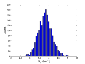
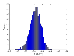
Figure 4: Histogram for the $G_{1}$ transition amplitude (top) and transition amplitude (bottom) obtained from Monte-Carlo fits of Eq.( 40) at $\mbox{WE}_{1}$ for 2000 QCD parameter sets. They are based on 10% uncertainty given to all the QCD input parameters.

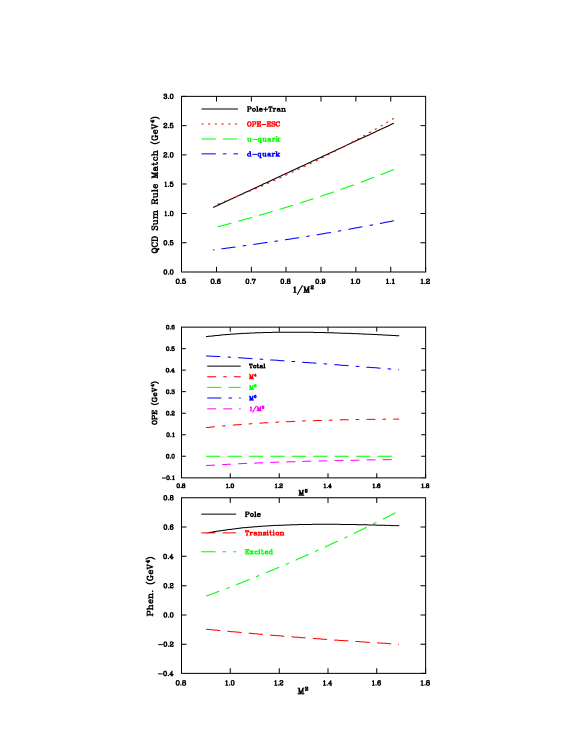
Figure 5: Analysis of the QCD sum rule in Eq. (40) (structure $\mbox{WE}_{1}$) for the proton at $\beta=-0.2$ according to Eq. (60). Top figure, the pole plus transition terms (solid lines) are compared against the OPE minus the excited-state contributions (dashed lines) as a function of $1/M^{2}$ (the two should match for an ideal sum rule). Also plotted are the individual contributions from u (long-dashed lines) and d (dot-dashed lines) quarks. Middle figure, the total in the OPE side and its various terms are plotted as a function of $M^{2}$. Bottom figure, the 3 terms in the phenomenological side: pole (solid), transition (long-dashed), and excited (dot-dashed) are plotted as a function of $M^{2}$.

To gain a better appreciation on how the QCD sum rules produce the results, we show some details of the analysis in Fig. 5, using the transition $p\gamma\to\Delta^{+}$ as an example. There are three graphs in this figure to give three different aspects of the analysis. The first graph shows how the two sides of Eq. (60) for this sum rule match over the Borel window, which should be linear as a function of $1/M^{2}$ according to the right-hand side of this equation. Indeed, we observe good linear behavior from the LHS (which is OPE-ESC). The slope is directly proportional to the transition amplitude $G_{1}$, and the intercept give the non-diagonal transition contribution $A$. We also plot the individual contributions from u and d quarks. We see that in this transition, the u-quark contribution is the dominant one, which is expected because it is doubled-represented in the proton ($uud$). In the next two graphs, we give details on the individual terms in the sum rule in Eq. (40), remembering that the sum rule is in the generic form of OPE-ESC=Pole+Transition. The second graph in Fig. 5 shows how the various terms contribute to the OPE as a function of $M^{2}$. The $M^{0}$ terms, which contain the contributions from the condensates $\chi a^{2}$ and $b$, play an important role. It is followed by the $M^{4}$ term which is the perturbative contribution. The $M^{2}$ term is zero in this channel because it is proportional to the strange quark mass. The $M^{-2}$ term gives a negative contribution and its contribution as a percentage of the entire OPE is about 10% at the lower end of the Borel window. In the third graph we show the three terms that comprise the phenomenological side (Pole, Transition, and ESC) as a function of $M^{2}$. The ground-state pole is dominant at the low end of the Borel window. The excited-state contribution starts small, then grows with $M^{2}$, as expected from the continuum model. The transition contribution is small in this sum rule. It is consistently smaller than the excited-state contribution and has a weak dependence on the Borel mass.

In our Monte-Carlo analysis, the entire QCD input phase space is mapped into the phenomenological output space, so we can also look into correlations between any two parameters by way of scatter plots of the two parameters of interest. Fig. 6 shows such an example. We see that the transition amplitude $G_{1}$ has a strong negative correlation with the vacuum susceptibility $\chi$. Larger $\chi$ (in absolute terms since $\chi$ is negative) leads to smaller $G_{1}$. Precise determination of the QCD parameters, especially those that have strong correlations to the output parameters, is crucial for keeping the uncertainties in the spectral parameters under control. We found similar strong correlations with $\chi$ in other transition channels.

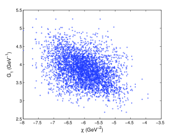
Figure 6: A scatter plot showing correlations between the transition amplitude $G_{1}$ and one of the QCD parameters $\chi$ for the $p\gamma\to\Delta^{+}$ at structure $\mbox{WE}_{1}$. It is obtained from 2000 Monte-Carlo samples with 10% uncertainty on all the QCD parameters.

V.2 The sum rule at $\mbox{WO}_{2}$

The sum rule at this structure is found in Eq. (53). We use the same procedure to analyze it. Since OPE expansion in this sum rule goes deeper than others (from $M^{2}$ to $1/M^{4}$), it is expected to be more reliable than the $\mbox{WO}_{1}$ sum rule. But our analysis shows that this advantage is offset by the smallness of the $1/M^{2}$ and $1/M^{4}$ terms. As a result, its performance is about the same as the sum rule at $\mbox{WE}_{1}$. Table 3 displays the results extracted from this sum rule.

Table 3: Similar to Table 2, but for the QCD sum rule in Eq. (53) (structure $\mbox{WO}_{2}$).

Transition	$\beta$	Window	$w$	A	$G_{1}$
		(GeV)	(GeV)	(GeV-3)	(GeV-1)
$p\gamma\to\Delta^{+}$	-0.2	0.9 to 1.2	1.3	-0.5(1)	3.52(32)
$n\gamma\to\Delta^{0}$	-0.2	0.9 to 1.2	1.35	0.5(1)	-3.68(33)
$\Sigma^{+}\gamma\to\Sigma^{*+}$	-0.2	1.2 to 1.6	1.4	0(1)	2.20(20)
$\Sigma^{0}\gamma\to\Sigma^{*0}$	-0.2	1.0 to 1.8	1.6	0.02(1)	0.92(10)
$\Sigma^{-}\gamma\to\Sigma^{*-}$	-0.2	1.0 to 1.6	1.6	-0.01(1)	-0.32(5)
$\Xi^{0}\gamma\to\Xi^{*0}$	-0.2	1.0 to 1.8	1.65	0.01(1)	-0.91(10)
$\Xi^{-}\gamma\to\Xi^{*-}$	-0.2	1.2 to 1.8	1.8	0(1)	0.21(3)
$\Lambda\gamma\to\Sigma^{*0}$	-0.2	1.0 to 1.6	1.45	0.05(1)	0.89(10)

V.3 The sum rule at $\mbox{WE}_{6}$

The sum rule is found in Eq. (49). This is the only sum rule that depends on $G_{2}$ alone. The results of our analysis are given in Table 4. The off-diagonal contributions (A) in the $p\to\Delta^{+}$ and $n\to\Delta^{0}$ are smaller by half than those for $G_{1}$, but the uncertainties are larger. They are small in the other channels, just like those for $G_{1}$. rediction, but others are not good. The reason of this is because he transition contribution ($A$) are as larger as the $G_{2}$ term, so the two terms can’t distinguish and get contaminated.

Table 4: Similar to Table 4, but for the $G_{2}$ amplitude from the QCD sum rule in Eq. (49) (structure $\mbox{WE}_{6}$).

Transition	$\beta$	Window	$w$	A	$G_{2}$
		(GeV)	(GeV)	(GeV-2)	(GeV-2)
$p\gamma\to\Delta^{+}$	-0.2	1.0 to 1.3	1.3	-0.26(4)	-2.34(48)
$n\gamma\to\Delta^{0}$	-0.2	1.0 to 1.3	1.3	0.26(4)	2.34(48)
$\Sigma^{+}\gamma\to\Sigma^{*+}$	-0.2	1.4 to 1.6	1.8	-0.07(1)	-0.41(45)
$\Sigma^{0}\gamma\to\Sigma^{*0}$	-0.2	1.5 to 1.8	1.5	-0.01(1)	-0.31(16)
$\Sigma^{-}\gamma\to\Sigma^{*-}$	-0.2	1.2 to 1.6	1.8	0.01(1)	-0.32(12)
$\Xi^{0}\gamma\to\Xi^{*0}$	-0.2	1.5 to 1.8	1.8	0.03(1)	0.38(29)
$\Xi^{-}\gamma\to\Xi^{*-}$	-0.2	1.4 to 1.8	1.9	0(1)	0.18(7)
$\Lambda\gamma\to\Sigma^{*0}$	-0.2	1.0 to 1.3	1.45	-0.09(1)	-0.62(17)

V.4 Individual quark contributions

To gain a deeper understanding of the dynamics, we consider the individual quark sector contributions to the transition amplitudes. In our approach, we can easily dial individual quark contributions to the QCD sum rules. For example, to turn off all u-quark (d-quark) contributions, we set the charge factor $e_{u}=0$ ($e_{d}=0$). To turn off all s-quark contributions, we set $e_{s}=0$, $m_{s}=0$, $f=1$, and $\phi=1$. We can extract a number corresponding to each quark contribution from the slope of Eq. (60) as a function of $1/M^{2}$, while keeping other factors the same ($\beta$, Borel window, $w$). We call this the raw individual quark contributions to the transition amplitudes. Table 5 gives the results for the $G_{1}$ amplitude from such a study. We see that the u-quark contribution in the transition $p\gamma\to\Delta^{+}$ is twice the d-quark contribution as expected, and both contributions are positive. It is the opposite in the transition $n\gamma\to\Delta^{0}$. The s-quark contribution is positive in the $\Sigma$ transitions, and negative in the $\Xi$ and $\Lambda$ transitions. In the $\Sigma^{0}\gamma\to\Sigma^{*0}$ channel, the d-quark and s-quark contributions largely cancel.

Table 5 gives the results for the $G_{2}$ amplitude. Similar pattern is observed in the proton and neutron channels, albeit the signs are opposite for $G_{1}$ and $G_{2}$. The s-quark contribution is opposite to that in $G_{1}$: negative in the $\Sigma$ channels and positive in the $\Xi$ channels. It donimates in the $\Sigma$ channels over the u-quark and d-quark contributions. Interestingly, s-quark contribution is exactly zero in the $\Lambda$ channel.

Table 5: Individual quark contributions to the transition amplitude $G_{1}$ in units of GeV^-1 extracted from the QCD sum rules in Eq. (40) (structure $\mbox{WE}_{1}$).

	$G_{1}^{u}$	$G_{1}^{d}$	$G_{1}^{s}$	$G_{1}^{tot}$
$p\gamma\to\Delta^{+}$	2.56(25)	1.28(13 )	0	3.84(38)
$n\gamma\to\Delta^{0}$	-1.28(13)	-2.56(25)	0	-3.84(38)
$\Sigma^{+}\gamma\to\Sigma^{*+}$	2.06(17)	0	0.69(6)	2.75(22)
$\Sigma^{0}\gamma\to\Sigma^{*0}$	1.00(9)	-0.50(5)	0.67(6)	1.17(10)
$\Sigma^{-}\gamma\to\Sigma^{*-}$	0	-1.04(8)	0.71(6)	-0.33(6)
$\Xi^{0}\gamma\to\Xi^{*0}$	-0.71(6)	0	-0.25(2)	-0.97(7)
$\Xi^{-}\gamma\to\Xi^{*-}$	0	0.37(3)	-0.27(2)	0.11(2)
$\Lambda\gamma\to\Sigma^{*0}$	1.91(16)	1.17(10)	-0.16(2)	2.92(25)

Table 6: Individual quark contributions to the transition amplitude $G_{2}$ in units of GeV^-2 extracted from the QCD sum rules in Eq. (49) (structure $\mbox{WE}_{6}$).

	$G_{2}^{u}$	$G_{2}^{d}$	$G_{2}^{s}$	$G_{2}^{tot}$
$p\gamma\to\Delta^{+}$	-1.57(32)	-0.77(10)	0	-2.34(48)
$n\gamma\to\Delta^{0}$	0.77(10)	1.57(32)	0	2.34(48)
$\Sigma^{+}\gamma\to\Sigma^{*+}$	-0.05(37)	0	-0.36(10)	-0.41(45)
$\Sigma^{0}\gamma\to\Sigma^{*0}$	-0.02(17)	0.01(8)	-0.32(9)	-0.31(16)
$\Sigma^{-}\gamma\to\Sigma^{*-}$	0	0.11(20)	-0.43(10)	-0.32(12)
$\Xi^{0}\gamma\to\Xi^{*0}$	0.15(24)	0	0.23(6)	0.38(29)
$\Xi^{-}\gamma\to\Xi^{*-}$	0	-0.08(12)	0.26(6)	0.18(7)
$\Lambda\gamma\to\Sigma^{*0}$	0.42(11)	0.20(6)	0	0.62(17)

V.5 Comparison with other theoretical calculations

The determination of N to $\Delta$ transition amplitudes has been made in a number of other theoretical approaches. In the following we briefly discuss each of these approaches in order to put our results from QCD sum rules in context. The discussion is by no means exhaustive, but indicative of the breadth of interest in these transition amplitudes. First, we present our results in Table 7 after converting from $G_{1}$ from structure $\mbox{WE}_{1}$ and $G_{2}$ from $\mbox{WE}_{6}$ into the various conventions discussed earlier, and compare them with those from a lattice QCD calculation Derek93 , a quark model calculation Darewych83 , and experiment PDG08 . For $G_{M1}$, we see that our results are slightly higher than those from lattice QCD and quark model calculations, but the overall pattern (in terms of magnitude and sign) is consistent among the three very different calculations. For the ratio $R_{EM}$, the results are very different. We predict negative values for all transitions at the level of 10% uncertainty. The lattice QCD results have too large errors to resolve the sign, although a more recent calculation in the $p\gamma\to\Delta^{+}$ channel gives a negative value alex08 . The quark model results have varying signs. It demonstrates the difficulty of quantifying the small deformation from spherical symmetry in these transitions.

Table 7: A comparison of N to $\Delta$ transition amplitudes from various approaches: this work (QCDSR) in three different conventions; lattice QCD Derek93 ; quark model Darewych83 , and experiment PDG08 .

Transition	QCDSR					Lattice QCD		Quark Model		Experiment
	$G_{M1}$	$R_{EM}$	$f_{M1}$	$A_{1/2}$	$A_{3/2}$	$G_{M1}$	$R_{EM}$	$G_{M1}$	$R_{EM}$	$G_{M1}$	$R_{EM}$
	$\mu_{B}$	%	GeV-1/2	GeV-1/2	GeV-1/2	$\mu_{B}$	%	$\mu_{B}$	%	$\mu_{B}$	%
$p\gamma\to\Delta^{+}$	4.30(43)	-1.66(17)	0.405	-0.19	-0.36	2.46(43)	3(8)	2.15	-0.009	3.02	-2.5(5)
$n\gamma\to \Delta^{0}$	-4.30(43)	-1.66 (17)	-0.405	0.19	0.36	-2.46(43)	3(8)	-2.15	-0.009
$\Sigma^{+}\gamma\to \Sigma^{*+}$	4.18 (42)	-2.85(29)	0.240	-0.11	-0.22	2.61(35)	5(6)	2.61	-0.210
$\Sigma^{0}\gamma\to \Sigma^{*0}$	1.79 (18)	-2.30 (23)	0.104	-0.05	-0.09	1.07(13)	4(6)	1.1	0.192
$\Sigma^{-}\gamma\to \Sigma^{*-}$	-0.53 (5)	-7.99 (8)	-0.031	0.01	0.03	-0.47(9)	8(4)	-0.4	0.985
$\Xi^{0}\gamma\to\Xi^{*0}$	-1.69(17)	-1.59(16)	-0.094	0.04	0.08	-2.77(31)	2.4(2.7)	-2.86	0.031
$\Xi^{-}\gamma\to \Xi^{*-}$	0.19 (2)	-12.42 (13)	0.010	0.00	-0.01	0.47(8)	7.4(3.0)	0.44	-0.259
$\Lambda\gamma\to\Sigma^{*0}$	3.34(34)	-4.62(48)	0.314	-0.135	-0.285

Since $p\gamma\to\Delta^{+}$ is the channel most widely studied and the only one measured in experiments, we give a more detailed comparison including more theoretical determinations. Fig. 7 summarizes the calculations of the magnetic dipole transition amplitude $G_{M1}$ in units of nucleon magneton. The calculations are grouped into six catagories: lattice QCD (Latt.), QCD sum rules results from this work (QCDSR), light-cone QCD sum rules (LCSR), hedgehog models including Skyrme and hybrid models (Skyrme), quark model calculations (Q.M), and bag models (Bag). The experimental result from the PDG is also displayed (Expt.). Fig. 8 summarizes the calculations of the ratio $R_{EM}$ in the same channel.

Figure 7: A comparison of the magnetic dipole transition amplitude $G_{M1}$ in units of nucleon magnetons in the $p\gamma\to\Delta^{+}$ transition from different approaches. See text for discussions.

Figure 8: A comparison of the $R_{EM}$ ratio in the $p\gamma\to\Delta^{+}$ transition. See text for discussions.

There are only a few lattice QCD calculations. The original one by Leinweber et. al. Derek93 obtained good signals for $G_{M1}$, but barely a signal for $R_{EM}$ ($+3\pm 8$ %), and no signal for $G_{C2}$. Shown here are the more recent calculations by Alexandrou et. al. which obtained reasonable signals for all three form factors. For $G_{M1}$, from top down, in units of nucleon magneton ($\mu_{N}$), the results are $2.5\pm 0.4$ Derek93 with a quenched Wilson action; $1.68\pm 0.06$ with a hybrid action, $1.48\pm 0.04$ with a quenched Wilson action, and $1.07\pm 0.04$ with a 2-flavor Wilson action alex08 . Strictly speaking, we should compare results at the chiral limit and $Q^{2}=0$. The lattice results quoted are at pion mass of around 400 MeV and non-zero momentum transfer. For the ratio $R_{EM}$, the results are $-4.1\pm 1.4$% alex04 at $Q^{2}=0.13$ GeV² extrapolated to the chiral limit in quenched QCD; and $-0.77\pm 0.88$% alex08 at $Q^{2}=0.04$ GeV² and $m_{\pi}=360$ MeV in full QCD with a hybrid action. The lattice signals for the transition form factors are by now well establsihed. With increasing computing power and better lattice technology, lattice calculations offer the best promise for precision determination of the transitions from QCD.

The two numbers for QCDSR are from different sum rules: the top one correponds to $G_{1}$ from WE₁ and $G_{2}$ from WE₆, the bottom one correponds to $G_{1}$ from WO₂ and $G_{2}$ from WE₆. They are converted to $G_{M1}$ and $R_{EM}$ for comparison.

The ligh-cone QCD results come from Ref. Rohrwild07 which involve photon distribution amplitudes (light-cone wavefunctions) up to twist 4.

The hedgehog models from top down include the holographic QCD calculation by Grigoryan, Lee and Yee Grigoryan09 which can be considered as a 5D version of the Skyrme model; the SU(3) Skyrme model calculation by Chemtob Chemtob85 ; the SU(2) Skyrme model calculations by Kunz and Mulders  Kunz90 ; and the SU(2) Skyrme model calculation by Adkins, Nappi and Witten Adkins83 . The semiclassical hedgehog calculation of Cohen and Broniowski Cohen86 gives a negative value (-2.8) for M1 moment so it is not shown in Fig. 7. Skyrme models produce reasonable results for the M1 amplitude, but vanishing ones for eletric quadrupole E2 transition matrix elements so they are left out in Fig. 8.

The quark model results include (from top down): a calculation by Franklin Franklin02 (It has been correlated with $G_{A}$ and provides arguably the best constraint on $G_{M1}$ in quark-model calculations); a Bethe-Salpeter determination from Mitra and Mittal Mitra ; a calculation by Guiasu and Koniuk Guiasu87 in which mesonic dressings of the nucleon are explicitly included; a calculation by Capstick  Capstick92 in which configuration mixing in the baryon SU(6) wave functions is accounted for; and a calculation by Darewych et. al. Darewych83 based on the simple quark model. Quark model calculations generally give small values for $R_{EM}$.

The bag models include a chiral bag calculation (top) by Kalbermann and Eisenberg Kalber , and an old MIT bag calculation (bottom) by Donoghue et. al. Donoghue .

VI Conclusion

We have carried out a comprehensive study of the $N\gamma\to\Delta$ transition amplitudes using the method of QCD sum rules. We derived a new, complete set of QCD sum rules using generalized interpolating fields and examined them by a Monte-Carlo analysis. Here is a summary of our findings.

We proposed a new way of extracting the transition amplitudes from the slope of straight lines as a function of $1/M^{2}$ in conjunction with the corresponding mass sum rules, as defined in Eq. (60). We find that this method is more robust than from looking for ‘flatness’ as a function of Borel mass. The linearity displayed from the OPE side matches well with the phenomenological side in most cases. The method also demonstrates clearly the role of the non-diagonal transition terms in the intermediate states caused by the external field: wherever such transitions are large, the corresponding sum rules perform poorly.

Of the 96 sum rules we derived (from 12 independent structures, each for 8 transitions), we find that the sum rules from the $\mbox{WE}_{1}$ and $\mbox{WO}_{2}$ structures are the most reliable for the transition amplitude $G_{1}$, based on OPE convergence and ground-state pole dominance, and smallness of the non-diagonal transitions. The QCD sum rules from these structures are in Eq. (40) and Eq. (53); their predictions are found in Table 2 and Table 3. Our attempt to extract the $G_{2}$ amplitude was less successful. The only sum rules that can give stable results are in Eq. (49) from structure $\mbox{WE}_{6}$. Their predictions are found in Table 4. Our final results in the various conventions are found in Table 7.

Our Monte-Carlo analysis revealed that there is an uncertainty on the level of 10% in the transition amplitudes if we assign 10% uncertainty in the QCD input parameters. It goes up to about 30% if we adopt the conservative assignments that have a wide range of uncertainties in Ref. Derek96 . The Monte-Carlo analysis also revealed some correlations between the input and output parameters. The most sensitive is the vacuum susceptibility $\chi$. So a better determination of this parameter can help improve the accuracy on the transition amplitudes and other quantities computed from the same method. We also isolated the individual quark contributions to the transition amplitudes. These contributions provide insight into the effects of SU(3)-flavor symmetry breakings in the strange quark, and environment sensitivity of quarks in different baryons.

We compared our results with a variety of theoretical calculations, and with experiment in the proton channel. Our result for transition amplitude $G_{M1}$ is larger than the experiment and other calculations, while our result for the ratio $R_{EM}$ is consistent with experiment. In general, we find that $G_{1}$ amplitudes are more stable than $G_{2}$ amplitudes in this approach. Our results for the $\Lambda\gamma\to\Sigma^{*0}$ transition are new.

Overall, the results for the N to $\Delta$ transition amplitudes in the QCD sum rule approach are not as robust as those for the baryon magnetic moments Wang08 ; Lee98b ; Lee98c . It is in large part due to the intrinsic un-equal mass double pole in the phenomenological representation of the spectral functions. Nonetheless, the calculations offer a physically-transparent, QCD-based perspective on the transitions in terms of quarks, gluons and vacuum condensates.

- (1) D. B. Leinweber, T. Draper, R. M. Woloshyn, Phys. Rev. D 48, 2230-2249 (1993).
- (2) C. Alexandrou, Ph. de Forcrand, Th. Lippert, Phys. Rev. D 69, 114506 (2004).
- (3) C. Alexandrou et. al., Phys. Rev. D 77, 085012 (2008).
- (4) M. A. Shifman, A. I. Vainshtein and Z. I. Zakharov, Nucl. Phys. B147, 385, 448 (1979). This paper is a top 10 all-time favorite in high energy physics with 3185 citations and counting.
- (5) B. L. Ioffe and A. V. Simlfa, Nucl. Phys. B232, 109, (1984).
- (6) J. Rohrwild, Phys. Rev. D 75, 074025 (2007).
- (7) T. M. Aliev and A. Ozpineci, Nucl. Phys. B 732 (2006) 291.
- (8) V. M. Belyaev and A. V. Radyushkin, Phys. Rev. D 53, 6509 (1996).
- (9) V. M. Braun, A. Lenz, G. Peters and A. V. Radyushkin, Phys. Rev. D 73, 034020 (2006)
- (10) L. Wang and F.X. Lee, Phys. Rev. D 78, 013003 (2008).
- (11) H. F. Jones, M. D. Scadron, Ann. of Phys. 81, 1 (1973).
- (12) Particle Data Group: C. Amsler et al., Phys. Lett. B667, 1 (2008).
- (13) N. F. Sparveris et al., Phys. Lett. B 651, 102 (2007).
- (14) R. M. Davidson, N. C. Mukhopadhyay, Phys. Rev. Lett. 79, 4509 (1997).
- (15) G. Blanpied et al., Phys. Rev. Lett. 79, 4337 (1997).
- (16) K. Joo et al., Phys. Rev. Lett. 88, 122001 (2002).
- (17) C. Mertz et al., Phys. Rev. Lett. 86, 2963 (2001).
- (18) T. Sato and T. S. H. Lee, Phys. Rev. C 54, 2660 (1996).
- (19) D. Drechsel et al., Nucl. Phys. A 645, 145 (1999).
- (20) R.A. Arndt, W.J. Briscoe, I.I. Strakovsky, R.L. Workman, Phys. Rev. C 66, 055213 (2002).
- (21) B. L. Ioffe, Nucl. Phys. B188, 317 (1981); Z. Phys. C 18, 67 (1983).
- (22) J. Pasupathy, J. P. Singh, S. L. Wilson, and C. B. Chiu, Phys. Rev. D 36, 1442 (1986).
- (23) S. L. Wilson, J. Pasupathy, C. B. Chiu, Phys. Rev. D 36, 1451 (1987).
- (24) F. X. Lee and X. Liu, Phys. Rev. D 66, 014014 (2002).
- (25) F. X. Lee, Phys. Rev. C 57, 322 (1998).
- (26) C. B. Chiu, J. Pasupathy and S. J. Wilson, Phys. Rev. D 33, 1961, (1986).
- (27) F. X. Lee, Phys. Rev. D 57, 1801 (1998).
- (28) F. X. Lee, Phys. Lett. B419, 14 (1998).
- (29) M. Sinha, A. Iqubal, M. Dey and J. Dey, Phys. Lett. B610, 283 (2005).
- (30) P. Ball, V. M. Braun and N. Kivel, Nucl. Phys. B 649, 263 (2003).
- (31) J. Rohrwild, JHEP 0709, 073 (2007).
- (32) D. B. Leinweber, Ann. of Phys. 254, 328 (1997).
- (33) S. Narison Phys. Lett. B666 455 (2008).
- (34) H.R. Grigoryan, T.-S.H. Lee, H.-U. Yee, arXiv:0904.3710 [hep-ph].
- (35) M. Chemtob, Nucl. Phys. B256, 600 (1985).
- (36) J. Kunz and P. J. Mulders, Phys. Rev. D 41, 1578 (1990).
- (37) G. S. Adkins, C. R. Nappi, and E. Witten, Nucl. Phys. B288, 552 (1983).
- (38) T. D. Cohen and W. Broniowski, Phys. Rev. D 34, 3472 (1986).
- (39) J. Franklin, Phys. Rev. D 66, 033010 (2002).
- (40) A. Mitra and A. Mittal, Phys. Rev. D 29, 1399 (1984).
- (41) H. Guiasu and R. Koniuk, Phys. Rev. D 36, 2757 (1987).
- (42) S. Capstick, Phys. Rev. D 46, 1965 (1992).
- (43) J. W. Darewych, M. Horbatsch, and R. Koniuk, Phys. Rev. D 28, 1125 (1983).
- (44) G. Kalbermann and J. M. Eisenberg, Phys. Rev. D 28, 71 (1983).
- (45) J. F. Donoghue, E. Golowich, and B. R. Holstein, Phys. Rev. D 12, 2875 (1975).