Correlators of supersymmetric Wilson-loops, protected operators and matrix models in ${\cal N}=4$ SYM

Abstract:

We study the correlators of a recently discovered family of BPS Wilson loops in ${\cal N}=4$ supersymmetric $U(N)$ Yang-Mills theory. When the contours lie on a two-sphere in the space-time, we propose a closed expression that is valid for all values of the coupling constant $g$ and for any rank $N$, by exploiting the suspected relation with two-dimensional gauge theories. We check this formula perturbatively at order ${\cal O}(g^{4})$ for two latitude Wilson loops and we show that, in the limit where one of the loops shrinks to a point, logarithmic corrections in the shrinking radius are absent at ${\cal O}(g^{6})$. This last result strongly supports the validity of our general expression and suggests the existence of a peculiar protected local operator arising in the OPE of the Wilson loop. At strong coupling we compare our result to the string dual of the ${\cal N}=4$ SYM correlator in the limit of large separation, presenting some preliminary evidence for the agreement.

1 Introduction

The supersymmetric Maldacena-Wilson [1, 2] loops in ${\cal N}=4$ supersymmetric Yang-Mills theory (SYM) were recently generalized to include a class of contours contained in an $S^{3}$, which also include a path-dependent coupling to the scalar fields of the theory [3, 4]. A subset of those Wilson loops are contained in a great $S^{2}$ and their discoverers pointed out an exact solvability and a potential connection to QCD₂ [3, 5]. These loops are given by (we consider our $S^{2}$ in hyperplane $x^{0}=0$)

$$W=\frac{1}{N}\text{Tr}{\cal P}\exp\oint d\tau\,\left(i\,\dot{x}^{i}A_{i}+\epsilon_{ijk}\,x^{j}\dot{x}^{k}\,M^{i}_{I}\,\Phi_{I}\right)$$ (1)

where $x^{i}(\tau)$ (where $i=1,\ldots,3$, $I=1,\ldots,6$) is a closed path on $S^{2}$, and $M^{i}_{I}$ is a $3\times 6$ matrix satisfying $MM^{T}=1$ and which we will take to be $M^{i}_{i}=1/R$ (no summation implied and $R$ is the $S^{2}$ radius) and all other entries zero. At the level of the vacuum expectation value (VEV) there is considerable evidence that

$$\langle W\rangle=\frac{1}{N}L_{N-1}^{1}\left(-g^{2}\,\frac{{\cal A}_{1}{\cal A}_{2}}{{\cal A}^{2}}\right)\exp\left(g^{2}\,\frac{{\cal A}_{1}{\cal A}_{2}}{2{\cal A}^{2}}\right),$$ (2)

where ${\cal A}_{1}$ is the area on the sphere enclosed by the Wilson loop, while ${\cal A}={\cal A}_{1}+{\cal A}_{2}$ is the total sphere area. To begin with, the 1/2 BPS circle (given by an equator) has been proved to be given by (2) [6, 7, 8] and there are strong arguments in favour of the 1/4 BPS circle of [9] (given by a latitude) also being captured by (2). At ${\cal O}(g^{2})$, (2) was proven for general contours in [3, 4]. This result was further confirmed at ${\cal O}(g^{4})$ in [10, 11]. The significance of the result is that it agrees with the calculation of the VEV of the Wilson loop in QCD₂ on an $S^{2}$ in the zero instanton sector [12] with the couplings related by

$$g_{2d}^{2}=-\frac{g^{2}}{\cal A}.$$ (3)

The idea that a class of ${\cal N}=4$ SYM Wilson loops might be exactly solvable and equivalent to Wilson loops in a lower dimensional theory is very attractive, and hints at a relationship between two very different quantum field theories. More specifically one could infer that the localization procedure presented in [8] could also apply to this more general class, pointing towards the existence of a sector of non-local topological observables in ${\cal N}=4$ SYM. Standard field theoretical arguments should then suggest the presence of protected local operators arising in the OPE of the Wilson loop (see [13] for related research in this direction).

To substantiate these ideas we need to go beyond the level of the one-point function of Wilson loops and consider correlators of loops. A first step in this direction was undertaken in [11], where a perturbative computation of the correlator of two latitudes at order ${\cal O}(g^{6})$ was undertaken. Lacking a zero-instanton QCD₂ result to compare to, in [11] the generalization to $S^{2}$ of the Wu-Mandelstam-Leibbrandt (WML) [14, 15, 16] prescription for QCD₂ in the plane proposed in [3, 4] was used. Indeed, this prescription has been recently shown to be equivalent to the zero-instanton QCD₂ result [36].

In the present paper we derive a general formula for correlators of BPS Wilson loops with arbitrary contours on $S^{2}$ in terms of the multi-matrix model governing the zero instanton expansion of QCD₂. The result is valid for any coupling constant $g$ and for any value of $N$: we compute explicitly the matrix integral for the correlator of two loops. Our general expression survives a series of non-trivial tests. First of all we calculate in ${\cal N}=4$ perturbation theory the correlator of two latitude Wilson loops at ${\cal O}(g^{4})$, finding perfect agreement with the matrix model result. Next we provide compact formulas for the perturbative ${\cal O}(g^{6})$ contribution, generalizing the results of [10], from which a numerical evaluation can be easily performed (we will report on this point in the future [18]). Here we prefer instead to investigate analytically the limit where one of the two latitudes shrinks to zero size: because our nonperturbative formula is an order by order polynomial in the shrinking radius, the absence of logarithmic terms is a crucial test of the matrix representation. We find indeed the absence of leading logarithms in the shrinking radius, a quite non-trivial result, differing dramatically from the analogous computation of non-BPS correlators [19] where logs are present.

Interestingly, by analyzing the OPE of the shrinking Wilson loop one can relate the absence of the logarithmic terms to the protection of a local operator which may be expressed as the trace of the square of a twisted field strength. Work [13] concerning super-protected local operators could be extended to also include this novel operator, which is based on very similar symmetries. We discuss this issue in section 2.

Armed with our general result we can therefore take the large $N$ and strong coupling limit and try to compare it to the ${\cal N}=4$ correlator from the string side. In the limit that the two latitudes shrink to opposite poles on the sphere, this calculation reduces to the semi-classical exchange of supergravity (SUGRA) modes between the two string worldsheets describing the Wilson loops at strong coupling. We find that at leading order in the large-separation limit, the matrix model result seems to capture the exchange of the SUGRA modes dual to a certain chiral primary operator. Other modes, dual to other protected operators present in the weak coupling OPE, should also be carefully included to test definitively this result at strong coupling. We find moreover an intriguing pattern of matching between the QCD₂ result and the exchange of heavier modes dual to chiral primary operators of higher dimension, which seems to extend to arbitrary order in the large-separation expansion. We have not yet understood the meaning of this highly non-trivial pattern of matching.

In this paper we present a survey of our investigations, deferring a complete analysis with all the relevant technical details to a future publication.

Note added: as this manuscript was being completed [20] appeared, presenting a partial overlap with the results of this paper.

2 Symmetries of the loops and of their correlators

We start by considering ${\cal N}=4$ SYM Wilson loops that are a special case of the general construction presented in [3, 4]. They are 1/4 BPS supersymmetric loops with the contour defined on a latitude of $S^{2}$, first put forward in [9]. Writing the Wilson loop as

$$W=\frac{1}{N}\text{Tr}{\cal P}\exp\oint d\tau\,\left(i\,\dot{x}^{\mu}A_{\mu}+|\dot{x}|\,\Theta^{I}\,\Phi_{I}\right),$$ (4)

the latitudes are given by the following closed paths on an $S^{2}\subset\mathbb{R}^{4}$ and on another $S^{2}\subset S^{5}$ which gives the coupling to the scalar fields $\Phi_{I}$ ($\mu=1,\ldots,4$, $I=1,\ldots,6$),

$$x^{\mu}=R\,(\sin\theta_{0}\cos\tau,\sin\theta_{0}\sin\tau,\cos\theta_{0},\,0),\ \ \ \ \Theta^{I}=(-\cos\theta_{0}\cos\tau,-\cos\theta_{0}\sin\tau,\sin\theta_{0},\,0,\,0,\,0).$$

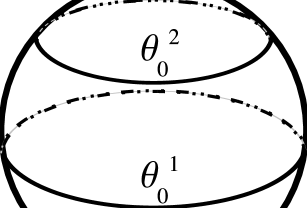
Figure 1: Two Wilson loops given by latitudes at polar angles $\theta_{0}^{1}$ and $\theta_{0}^{2}$.

Two such Wilson loops are pictured in figure 1. The supersymmetries preserved by these operators are fully described in [3], see section 2.3.1: here we just repeat some details of that analysis which are relevant to our work.

Under general superconformal transformations we have for the ${\cal N}=4$ SYM bosons

$$\delta_{\epsilon}A_{\mu}=\bar{\Psi}\gamma_{\mu}\,\epsilon,\qquad\delta_{\epsilon}\Phi_{i}=\bar{\Psi}\Gamma_{i}\,\epsilon,\quad\epsilon=\epsilon_{0}+x^{\mu}\gamma_{\mu}\epsilon_{1}.$$ (5)

Demanding that $\delta_{\epsilon}W=0$ one finds two relations

$$\begin{split}&\gamma_{12}\,\epsilon_{1}=-\Gamma_{12}\,\epsilon_{1},\\ &\Gamma_{3}\,\epsilon_{0}=\Bigl{[}i\gamma_{12}+\cos\theta_{0}\,\gamma_{3}\Gamma_{2}(\gamma_{23}+\Gamma_{23})\Bigr{]}\epsilon_{1}.\end{split}$$ (6)

It is clear that each of them reduce the supersymmetry by half, and therefore a single latitude is 1/4 BPS. We will be mainly interested in the correlator of two such Wilson loops, as shown in figure 1. The first relation in (LABEL:latsusy) is shared between two such latitudes, whereas the second is clearly not. Thus two latitudes are collectively 1/8 BPS, each sharing half of their individual supersymmetry. The same reasoning applies of course to a collection of $n$ latitudes, resulting always in a 1/8 BPS system.

2.1 Operator product expansion

In the next section we will present results of a perturbative calculation of the correlator of two latitudes and, in particular, we will consider the limit where one of the latitudes shrinks to a point at the pole of the sphere. The emerging structure can be usefully understood in terms of the OPE and its physical meaning is quite transparent.

The crucial observation is that, viewed from a comparably large distance, the unshrunken Wilson loop sees the shrunken loop as a collection of local operators [21]: the quantum behavior is encoded into Wilson coefficients and anomalous dimensions. The story was worked out in detail for two circular Wilson-Maldacena loops in [19]. Here, for the 1/4 BPS latitude, we will find that the relevant OPE is quite different, giving rise to novel operators which appear to have protected dimensions.

When analysing the OPE, we can in fact consider the general situation of loops with $arbitrary$ contours on $S^{2}$ that are generically 1/8 BPS. As noticed in [3] the Wilson loop (1) can be written in terms of a new gauge connection

$${\cal A}_{i}=A_{i}+i\epsilon_{ijk}\,x^{j}\,\frac{\Phi^{k}}{R}.$$ (7)

The OPE expansion will appear particularly simple using this generalized connection. The first step is to determine the classical expansion of our Wilson loops in terms of local gauge-invariant operators when the circuit is small. To achieve this goal we shall assume that the circuit can be written as follows

$$x^{i}(t)=x_{0}^{i}+r\hat{x}^{i}(t),$$ (8)

$x_{0}$ being the point about which the loop is shrinking and $r$ a parameter that will control the limit. We expand the contour integral by exploiting the Fock-Schwinger gauge $(x-x_{0})^{i}{\cal A}_{i}(x)=0$, where the following formula holds in terms of the new gauge curvature ${\cal F}_{ji}$

$${\cal A}_{i}(x)=\int_{0}^{1}d\lambda\lambda(x-x_{0})^{j}{\cal F}_{ji}(x_{0}+\lambda(x-x_{0})).$$ (9)

The leading order result is given by

$$\begin{split}\oint_{C}dt{\cal A}_{i}(x)\dot{x}^{i}=&\frac{r^{2}}{2}{\cal F}_{ij}(x_{0})\oint_{C}dt\hat{x}^{i}(t)\dot{\hat{x}}(t)+O(r^{3})=\frac{r^{2}}{2}\epsilon^{ijk}{\cal F}_{ij}(x_{0})n_{k}(x_{0})+O(r^{3}),\end{split}$$ (10)

$n_{i}(x_{0})$ being a normal vector to $S^{2}$ at the point $x_{0}$, depending on $x_{0}$ and the contour. The expansion could of course be extended to any given order in $r$, producing a series of local operators $O^{J}_{C}(x)$ determined by the particular shape of the Wilson loop, the generalized connection ${\cal A}_{i}$ itself depending on the contour. Because these operators should share the BPS properties of the associated Wilson loop, we obtain a practical realization of the proposal of [13]: in particular we could expect that their correlation functions, when restricted to the relevant $S^{2}$, are somehow protected from quantum corrections. This would imply severe constraints on Wilson loop correlators. Let us exemplify the consequences for latitude correlators (we will consider here for simplicity the $SU(N)$ case).

In our specific example we take as our shrinking point the north pole, $x_{0}=R(0,0,1)$, while $r=\sin\theta_{0}$ and $\hat{x}^{i}(t)=R(\cos t,\sin t,\tan\frac{\theta_{0}}{2})$. Due to the trace in the path-exponential the first non-vanishing contribution to the OPE is quadratic in the fields, and we get explicitly at leading order

$$W_{0}=1+\frac{\pi^{2}\sin\theta_{0}^{4}}{2N}\,{\cal O}_{\cal F}(x_{0})$$ (11)

where

$$\mathcal{O}_{\cal F}(x_{0})=\text{Tr}\Bigl{[}2R\,\Phi_{3}-iR^{2}\,F_{12}-R^{2}\,(\partial_{1}\Phi_{1}+\partial_{2}\Phi_{2})\Bigr{]}^{2}.$$ (12)

We note a peculiar feature that makes this OPE quite different from the usual circular Wilson-Maldacena case [19]: operators of classical dimension 2, 3, and 4 all couple with the same power of the parameter which sets the size of the shrinking latitude: the polar angle $\theta$ (in the standard case the power is the classical dimension itself). Indeed the overall scale $R$ of the $S^{2}$ is just a place keeper. The conformality of ${\cal N}=4$ SYM prevents it from playing any rôle, and it drops out of the calculation of any observable.

We notice that we can easily obtain the leading term of the two latitude correlator at order $g^{4}$ from the OPE (11), once we restore the canonical normalization for the fields. We just need to compute the correlation function

$$\langle{\cal O}_{\cal F}(x_{0})\oint dt\,\left(\,\dot{x}_{1}^{i}A_{i}(x_{1})-i\epsilon_{ijk}\,x_{1}^{j}\dot{x}_{1}^{k}\,\Phi^{i}(x_{1})\right)\rangle=i\frac{\cos\left(\theta_{1}\right)+1}{4\pi},$$ (13)

that enters in the Wick contraction. Taking the relevant color traces we get

$$\frac{\langle W_{0}W_{1}\rangle}{\langle W_{0}\rangle\langle W_{1}\rangle}-1=\frac{g^{4}}{8}\left(2\sin^{2}\frac{\theta_{0}}{2}\cos^{2}\frac{\theta_{1}}{2}\right)^{2}=\frac{g^{4}r^{4}}{32}\cos^{2}\frac{\theta_{1}}{2}.$$ (14)

The above result will be confirmed in the next section by the finite size correlator. Actually we can learn something more: the general expectation for the structure of the OPE of a shrinking Wilson loop is given by [19, 21, 24]

$$\frac{W}{\langle W\rangle}=1+\sum_{J}\,\xi_{J}(g^{2})\,L^{\Delta_{J}}\,O_{J}(x)$$ (15)

where $L$ is the size of the shrinking loop, and $O_{J}(x)$ is an operator of classical dimension $J$ and quantum dimension $\Delta_{J}=J+g^{2}\,\Delta_{J}^{(1)}+\ldots$. The Wilson coefficients $\xi_{J}(g^{2})$ depend on the coupling constant $g^{2}$. The curious structure of the latitude OPE is a reflection of the fact that the coefficients $\xi_{J}(g^{2})$ which describe the coupling of the Wilson loop to a specific operator $O_{J}(x)$ are themselves functions of $\theta$ [27], and can be expanded as $\xi_{J}(g^{2},\theta)=\sum_{k}\xi^{(k)}_{J}(g^{2})\,\theta^{k}$ in the limit $\theta\to 0$. This provides us with the general structure for the OPE of $W_{0}$

$$\begin{split}\frac{W_{0}}{\langle W_{0}\rangle}&=1+\sum_{J}\,\xi_{J}(g^{2},\theta_{0})\,\theta_{0}^{\Delta_{J}}\,O_{J}(x_{0})=1+\sum_{J,\,k}\,\xi^{(k)}_{J}(g^{2})\,\theta_{0}^{\Delta_{J}+k}\,O_{J}(x_{0})=\\ &=1+\xi^{(2)}_{2}\,\theta_{0}^{\Delta_{2}+2}\,O_{2}(x_{0})+\xi^{(1)}_{3}\,\theta_{0}^{\Delta_{3}+1}\,O_{3}(x_{0})+\xi^{(0)}_{4}\,\theta_{0}^{\Delta_{4}}\,O_{4}(x_{0})+\ldots\,,\end{split}$$ (16)

where we have dropped the scale $R$ (to restore it replace $O_{J}(x_{0})\to R^{\Delta_{J}}\,O_{J}(x_{0})$), and have noted the vanishing of $\xi_{2}^{(0,1)}$ and $\xi_{3}^{(0)}$ from the explicit expression of (12). The explicit form of $O_{2,3,4}(x_{0})$ is simply obtained from ${\cal O}_{\cal F}(x_{0})$. Actually there are multiple operators of the same classical dimension, so there is an extra suppressed index on the $\xi_{J}(g^{2},\theta_{0})$, $\Delta_{J}$, and $O_{J}(x_{0})$, which is implicitly summed over in (16). In the last line we are referring only to the operators appearing in (12) as these are the only ones present at leading order in $\theta_{0}$. We derive the following general relation in the shrinking limit

$$\begin{split}\frac{\langle W_{1}\,W_{0}\rangle}{\langle W_{1}\rangle\langle W_{0}\rangle}=&1+\xi^{(2)}_{2}\,\theta_{0}^{\Delta_{2}+2}\,\langle W_{1}\,O_{2}(x_{0})\rangle+\xi^{(1)}_{3}\,\theta_{0}^{\Delta_{3}+1}\,\langle W_{1}\,O_{3}(x_{0})\rangle+\xi^{(0)}_{4}\,\theta_{0}^{\Delta_{4}}\,\langle W_{1}\,O_{4}(x_{0})\rangle+\ldots\,.\end{split}$$ (17)

We notice that when expanded at small coupling the $\theta_{0}^{\Delta_{J}}$ terms generically produce logarithms $\theta_{0}^{\Delta_{J}}=\theta_{0}^{J}+g^{2}\,\Delta_{J}^{(1)}\,\theta_{0}^{J}\log\theta_{0}+\ldots$ if quantum corrections modify the classical dimensions. The quantities $\xi^{(2)}_{2}$, $\xi^{(1)}_{3}$, and $\xi^{(0)}_{4}$ may easily be read-off in our case from (12). Since the operators appearing in the explicit expression are quadratic in the fields, one has that $\xi^{(2)}_{2}$, $\xi^{(1)}_{3}$, and $\xi^{(0)}_{4}$ lead as $g^{4}$. We therefore generally expect terms of the form $g^{6}\log\theta_{0}$ to show up in the perturbative expansion of the correlator at order $g^{6}$, in the shrinking limit.

The presence of logarithmic corrections would be a signal that anomalous dimensions are playing a part, suggesting that the full interacting theory should be taken into account and localization techniques would not be sufficient in the exact computation. It would also rule out the relation with two-dimensional Yang-Mills that produces just polynomial dependence on $\theta$ at any order of perturbation theory, as we will see in section 4. In section 2 we show that, surprisingly, no such logarithmic terms appear at order $g^{6}$, supporting the matrix model proposal. This indicates that the composite operator ${\cal O}(x)$, arising from the OPE of the BPS loops (1), should be protected - at least at the first non-trivial quantum order. In other words logarithmic divergences should be absent in the two-point function $\langle\,{\cal O}(x_{1})\,{\cal O}(x_{2})\,\rangle$, when $x_{1,2}$ belong to the relevant $S^{2}$, in the same way as the operators defined in [13]. It is not difficult to show in fact that ${\cal O}(x)$ inherits the BPS properties of the latitude loop, and a certain amount of supersymmetry is preserved by its correlators.

3 Perturbative results on Wilson loop correlators

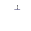
Figure 2: $g^{2}-$diagram

In this section we perform a perturbative analysis up to order $g^{6}$ for the connected correlator $\mathcal{W}(C_{1},C_{2})\equiv W(C_{1},C_{2})-W(C_{1})W(C_{2})$ of two latitudes in the case that the gauge group is $U(N)$. To begin with, we shall consider the $g^{2}$ diagram depicted in fig. 2. [Notice that this contribution would be absent in a $SU(N)$theory.]

In order to carry out the computation, we parameterize the two circuits using polar coordinates

$$\begin{split}C_{1}=&R(\sin\theta_{1}\cos\tau,\sin\theta_{1}\sin\tau,\cos\theta_{1})\\ C_{2}=&R(\sin\theta_{2}\cos\sigma,\sin\theta_{2}\sin\sigma,\cos\theta_{2}),\end{split}$$ (18)

and define the effective propagator $\Delta_{C_{1}C_{2}}(\tau,\sigma)$ connecting the two loops

$$\begin{split}\Delta_{C_{1}C_{2}}(\tau,\sigma)=&\frac{2}{N}\langle\text{Tr}(\mathcal{A})(\tau)\text{Tr}(\mathcal{A})(\sigma)\rangle_{0}=-\frac{\sin\theta_{1}\sin\theta_{2}\left(\cos\left(\tau-\sigma\right)\left(\cos\theta_{1}\cos\theta_{2}-1\right)+\sin\theta_{1}\sin\theta_{2}\right)}{8\pi^{2}\left(\cos\theta_{1}\cos\theta_{2}+\cos\left(\tau-\sigma\right)\sin\theta_{1}\sin\theta_{2}-1\right)},\end{split}$$ (19)

where $\mathcal{A}$ denotes the effective field $iA_{\mu}(x)\dot{x}^{\mu}+\!\Theta_{I}\Phi^{I}(x)|\dot{x}|$. Then the $g^{2}-$contribution is given by

$$\left.\mathcal{W}(C_{1},C_{2})\right|_{g^{2}}=\frac{g^{2}}{2N}\int_{0}^{2\pi}d\tau d\sigma~{}~{}\Delta_{C_{1}C_{2}}(\tau,\sigma)=\frac{\lambda}{N^{2}}\frac{A_{1}A_{2}}{A^{2}}\ \ \ \ \ \ \ (\lambda\equiv g^{2}N),$$ (20)

where $A$ is the total area of the sphere, and $A_{1}$ and $A_{2}$ are the areas enclosed by the two Wilson-loops given by

$$\frac{A_{1}}{A}=\frac{2\pi(1-\cos\theta_{1})}{4\pi}=\sin^{2}\frac{\theta_{1}}{2}\ \ \ \ \frac{A_{2}}{A}=\frac{2\pi(1+\cos\theta_{2})}{4\pi}=\cos^{2}\frac{\theta_{2}}{2}.$$ (21)

At order $g^{4}$, we have to consider the diagrams in fig. 3. First, we shall consider the contribution $S_{g^{2}-g^{2}}$ due to diagram $(b_{1})$. Its evaluation reduces to the following integral over the circuits

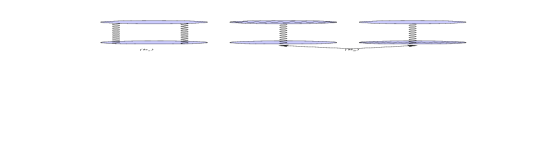
Figure 3: $g^{4}$ diagrams

$$S_{g^{2}-g^{2}}= \frac{g^{4}}{16}\int_{0}^{2\pi}\!\!\!\!\!d\tau_{1}d\tau_{2}d\sigma_{1}d\sigma_{2}\mbox{\small$\biggl{[}\Delta_{C_{1}C_{2}}(\tau_{1},\sigma_{1})\Delta_{C_{1}C_{2}}(\tau_{2},\sigma_{2})+\Delta_{C_{1}C_{2}}(\tau_{1},\sigma_{2})\Delta_{C_{1}C_{2}}(\tau_{2},\sigma_{1})\biggr{]}$}=$$

$$= \frac{g^{4}}{8}\left[\int_{0}^{2\pi}\!\!\!d\tau_{1}d\sigma_{1}\Delta_{C_{1}C_{2}}(\tau_{1},\sigma_{1})\right]^{2}=\frac{g^{4}}{8}\left[2\sin^{2}\frac{\theta_{1}}{2}\cos^{2}\frac{\theta_{2}}{2}\right]^{2}=\frac{\lambda^{2}}{2N^{2}}\frac{A_{1}^{2}A_{2}^{2}}{A^{4}}.$$ (22)

Next we shall consider the contribution $S_{g-g^{3}}$ due to the two diagrams $(b_{2})$. The sum of the two diagrams yields

$$S_{g-g^{3}}= \frac{g^{4}}{4!}\oint_{C_{1}}\!\!d\tau_{1}\oint_{C_{2}}\!\!d\sigma_{1}d\sigma_{2}d\sigma_{3}\mbox{\small$\left(\Delta_{C_{1}C_{2}}(\tau_{1},\sigma_{1})\Delta_{C_{2}C_{2}}(\sigma_{2},\sigma_{3})+\Delta_{C_{1}C_{2}}(\tau_{1},\sigma_{2})\Delta_{C_{2}C_{2}}(\sigma_{1},\sigma_{3})+\right.$}$$

$$\mbox{\small$\left.+\Delta_{C_{1}C_{2}}(\tau_{1},\sigma_{3})\Delta_{C_{2}C_{2}}(\sigma_{1},\sigma_{2})\right)$}+(C_{1}\leftrightarrow C_{2})=$$

$$= \frac{g^{4}}{16}\left(2\sin^{2}\frac{\theta_{1}}{2}\cos^{2}\frac{\theta_{2}}{2}\right)(\sin^{2}\theta_{1}+\sin^{2}\theta_{2})=\frac{\lambda^{2}}{2N^{2}A^{4}}A_{1}A_{2}(A_{1}A_{3}+A_{2}A_{3}+2A_{1}A_{2}),$$ (23)

where $\Delta_{C_{2}C_{2}}(\sigma_{i},\sigma_{j})=\frac{\sin^{2}\theta_{2}}{8\pi^{2}}$ and $A_{3}=A-A_{1}-A_{2}$. If we sum all the contributions at order $g^{4}$, the total result is

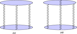
Figure 4: Triple-exchange: (a) planar diagram; (b) non-planar diagram.

$$\left.\mathcal{W}(C_{1},C_{2})\right|_{g^{4}}=\frac{\lambda^{2}}{2N^{2}A^{4}}A_{1}A_{2}({A}_{1}{A}_{3}+{A}_{2}{A}_{3}+3{A}_{1}{A}_{2}).$$ (24)

A remark on the $S_{g^{2}-g^{2}}$ contribution is in order. This is the only contribution in a $SU(N)$ theory and one can verify that its small $r-$expansion is in agreement with the OPE result [14], supporting the idea that the leading contribution to the Wilson-loop is determined only by $\mathcal{O}_{\cal F}$.

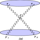
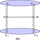
Figure 5: (a) X-diagram; (b) H-diagram.

We now come to considering the $g^{6}$ contribution. Since, at this order, the $\mathcal{N}=4$ interactions will start contributing, a complete analytic evaluation of all the relevant integrals is out of reach. However one can write compact formulas which can be used as a starting point for a numerical evaluation [18]. We shall exploit this possibility in a future paper. Here we shall instead be interested in singling out the coefficients of contributions of the form $r^{k}\log(r)$, potentially present in the evaluation of the connected correlator. The knowledge of these coefficients already provides non trivial information on the properties of the correlator. In fact, as explained in the previous section, a non-vanishing result for these coefficients would clash with the expectation that the correlator localizes.

For this computation, we limit our attention to the gauge group $SU(N)$ and we can separate the diagrams into two classes: the ladder diagrams and the interaction diagrams. The ladder diagrams are depicted in fig. 4 and it is easy to realize that they cannot generate any contribution of the form $r^{k}\log(r)$. They are actually analytic in the small $r-$limit. The contributions $r^{k}\log(r)$ are instead generated by the interactions diagrams in figs. 5 and 6. The origin of this non analytic behavior can be traced back to the small distance singularities appearing in the integration over the position of the vertices. Thus in order to extract these logarithmic singularities, we have to first perform these integrations analytically, and only after that can we expand in powers of the radius. To illustrate the procedure let us start by considering the $X$-diagram. Its expression can be cast into the following compact form

$$\begin{split}\mathbf{X}=\frac{\lambda^{3}}{8N^{2}}&\int_{0}^{2\pi}\!\!\!\!\!d\tau_{1}d\tau_{2}d\sigma_{1}d\sigma_{2}\left[(\dot{x}_{1}\circ\dot{y}_{2})(\dot{x}_{2}\circ\dot{y}_{1})-\right.\\ &\left.-(\dot{x}_{1}\circ\dot{x}_{2})(\dot{y}_{1}\circ\dot{y}_{2})\right]\mathcal{I}^{(4)}(x_{1},x_{2},y_{1},y_{2}),\end{split}$$ (25)

where $(\dot{x}\circ\dot{y})=\dot{x}\cdot\dot{y}-|\dot{x}||\dot{y}|\Theta_{\dot{x}}\cdot\Theta_{\dot{y}}$ with $|\dot{x}|\Theta_{\dot{x}}^{I}=M_{I}^{i}\epsilon_{irs}\dot{x}^{r}x^{s}$ and

$$\mathcal{I}^{(4)}(x_{1},x_{2},y_{1},y_{2})\equiv\frac{1}{(2\pi)^{8}}\int\frac{d^{4}w}{(x_{1}-w)^{2}(x_{2}-w)^{2}(y_{1}-w)^{2}(y_{2}-w)^{2}}.$$ (26)

Here and in the following $x_{i}\equiv x(\tau_{i})$ and $y_{i}\equiv y(\sigma_{i})$ will denote points on the upper and lower latitudes respectively (see fig. 1). The integration over $w$ in (26) can be performed and it is then straightforward to extract the singular part when we shrink the latitude $\theta=\theta_{1}$ to the north-pole of the sphere $S^{2}$ (see appendix $A$ for details.) The singular part is given by

$$\mathcal{I}^{(4)sing.}(x_{1},x_{2},y_{1},y_{2})=-\frac{{\log r}}{128\pi^{6}}\times$$

$$\times\!\int_{0}^{1}\!\!\frac{d\alpha}{\mbox{\small$(1-\alpha){(y_{1}-x_{2})^{2}(y_{2}-x_{1})^{2}}-\alpha(1-\alpha){(x_{1}-x_{2})^{2}(y_{1}-y_{2})^{2}}+{\alpha(y_{1}-x_{1})^{2}(y_{2}-x_{2})^{2}}$}},$$ (27)

where $r=\sin\theta_{1}$. The integration over the circuit is straightforward and can be evaluated by Taylor-expanding in $r$. At leading order we find that

$$\mathbf{X^{sing}}=\frac{5r^{4}\cos^{4}\left(\frac{\theta_{2}}{2}\right)\log(r)}{768\pi^{2}}+O(r^{5}).$$ (28)

Consider now the $H-$diagram in fig. (5). We can write the contribution from this diagram as follows

$$\begin{split}\mathbf{H}=&-\frac{\lambda^{3}}{8N^{2}}\int d^{4}w\left[\underset{\mathbf{A}_{1}}{{P}^{M}(x_{1},y_{1},w)\square_{w}{P}^{M}(x_{2},y_{2},w)}+\underset{\mathbf{B}_{1}}{{P}^{M}(x_{1},y_{1},w)\square_{w}{Q}^{M}(x_{2},y_{2},w)}+\right.\\ &\ \ \ \ \ \ \ \ \ \ \ +\left.\underset{\mathbf{B}_{2}}{{Q}^{M}(x_{1},y_{1},w)\square_{w}{P}^{M}(x_{2},y_{2},w)}+\underset{\mathbf{A_{2}}}{{Q}^{M}(x_{1},y_{1},w)\square_{w}{Q}^{M}(x_{2},y_{2},w)}\right],\end{split}$$ (29)

where

$$P^{M}(x_{i},y_{i},w)=\int_{0}^{2\pi}\!\!\!\!\!\!d\tau_{i}d\sigma_{i}\left[2\dot{y_{i}}^{M}(\dot{x}_{i}\cdot\partial_{{y_{i}}}\mathcal{I}_{i}(x_{i},y_{i},w))-2\dot{x}_{i}^{M}(\dot{y_{i}}\cdot\partial_{x_{i}}\mathcal{I}_{i}(x_{i},y_{i},w))\right]$$ (30)

and

$$Q^{M}(x_{i},y_{i},w)=\int_{0}^{2\pi}\!\!\!\!\!\!d\tau_{i}d\sigma_{i}(\dot{x}_{i}\circ\dot{y}_{i})(\partial_{x^{M}_{i}}\mathcal{I}_{i}(x_{i},y_{i},w)-\partial_{y^{M}_{i}}\mathcal{I}_{i}(x_{i},y_{i},w)).$$ (31)

In eqs. (29), (30) and (31), the index $M$ is a ten-dimensional label running from $1$ to $10$ and in particular we have defined $x^{M}\equiv(x^{\mu},i\Theta^{I}|\dot{x}|)$ and $\partial_{M}\equiv(\partial_{\mu},0)$. The function $\mathcal{I}_{1}(x_{i},y_{i},w)$ is defined by the scalar integral

$$\mathcal{I}_{1}(x_{i},y_{i},w)=\frac{1}{(2\pi)^{6}}\int\frac{d^{4}z}{(x_{i}-z)^{2}(y_{i}-z)^{2}(w-z)^{2}}.$$ (32)

The spatial components $P^{\mu}$ of $P^{M}$ satisfy the following two simple identities: $z_{\mu}P^{\mu}=\partial_{\mu}P^{\mu}=0$, as can easily be checked by direct computation. Moreover, for two latitudes parallel to the plane $(2,3)$, $P^{1}$ and $P^{4}$ trivially vanish. Since $P^{\mu}$ is a just a function of $z^{\mu}$, all these properties are consistent if and only if $P^{\mu}=0$. This result simplifies dramatically the computation for the correlator of two latitudes: in fact the contributions $\mathbf{B_{1}}$ and $\mathbf{B_{2}}$ in (29) are identically zero. Recall, in fact, that $Q^{M}$ is different from zero (by construction) only when $M$ is spatial. Thus we are just left with $\mathbf{A_{1}}$ and $\mathbf{A_{2}}$ to be computed.

Let us first compute first $\mathbf{A_{2}}$. It is convenient to rewrite this contribution as follows

$$\mathbf{A_{2}}=\frac{\lambda^{3}}{8N^{2}}\int_{0}^{2\pi}\!\!\!\!\!\!d\tau_{1}d\tau_{2}d\sigma_{1}d\sigma_{2}\dot{x}_{1}\circ\dot{y_{1}}\dot{x}_{2}\circ\dot{y_{2}}(\partial_{x_{1}}-\partial_{y_{1}})\cdot(\partial_{x_{2}}-\partial_{y_{2}})\mathcal{H}(x_{1},y_{1};x_{2},y_{2}),$$ (33)

where

$$\begin{split}\mathcal{H}(x_{1},y_{1};x_{2},y_{2})=&\frac{1}{(2\pi)^{10}}\int\frac{d^{4}zd^{4}w}{(x_{1}-z)^{2}(y_{1}-z)^{2}(z-w)^{2}(x_{2}-w)^{2}(y_{2}-w)^{2}}.\end{split}$$ (34)

The action of $(\partial_{x_{1}}-\partial_{y_{1}})\cdot(\partial_{x_{2}}-\partial_{y_{2}})$ on $\mathcal{H}(x_{1},y_{1};x_{2},y_{2})$ can then be evaluated with the identity (A.7) given in [25]. One finds

$$\begin{split}(\partial_{x_{1}}-\partial_{y_{1}})\cdot&(\partial_{x_{2}}-\partial_{y_{2}})\mathcal{H}(x_{1},y_{1};x_{2},y_{2})=\\ =&\frac{1}{(x_{1}-y_{1})^{2}(x_{2}-y_{2})^{2}}\left[\mathcal{I}^{(4)}(x_{1},y_{1},x_{2},y_{2})((x_{1}-x_{2})^{2}(y_{1}-y_{2})^{2}-(x_{1}-y_{2})^{2}(x_{2}-y_{1})^{2})+\right.\\ &+\left.\frac{1}{(2\pi)^{2}}(Y(x_{1},x_{2},y_{2})-Y(y_{1},x_{2},y_{2})+Y(x_{2},x_{1},y_{1})-Y(y_{2},x_{1},y_{1}))\right],\end{split}$$ (35)

where ${Y}(x_{1},x_{2},x_{3})\equiv{\mathcal{I}_{1}(x_{1},x_{2},x_{3})}[(x_{1}-x_{3})^{2}-(x_{1}-x_{2})^{2}].$ When the first latitude ($\theta=\theta_{1}$) is shrunk to zero the logarithmically divergent terms can be generated by $\mathcal{I}^{(4)}$ and by the $Y$ that depends both on $x_{1}$ and $x_{2}$. Therefore we can write

$$\begin{split}\mathbf{A_{2}^{sing.}}=&\frac{\lambda^{3}}{8N^{2}}\int_{0}^{2\pi}\!\!\!\!\!\!d\tau_{1}d\tau_{2}d\sigma_{1}d\sigma_{2}\frac{(\dot{x}_{1}\circ\dot{y_{1}})(\dot{x}_{2}\circ\dot{y_{2}})}{(x_{1}-y_{1})^{2}(x_{2}-y_{2})^{2}}\biggl{[}\mathcal{I}^{(4)sing.}(x_{1},y_{1},x_{2},y_{2})((x_{1}-x_{2})^{2}(y_{1}-y_{2})^{2}-\\ &-(x_{1}-y_{2})^{2}(x_{2}-y_{1})^{2})+\frac{1}{(2\pi)^{2}}(Y^{sing.}(x_{1},x_{2},y_{2})+Y^{sing.}(x_{2},x_{1},y_{1}))\biggr{]},\end{split}$$ (36)

where we have defined

$${Y}^{sing.}(x_{1},x_{2},y_{2})\equiv{\mathcal{I}_{1}^{sing.}(x_{1},x_{2},y_{2})}[(x_{1}-y_{2})^{2}-(x_{1}-x_{2})^{2}]$$

and

$${Y}^{sing.}(x_{2},x_{1},y_{2})\equiv{\mathcal{I}_{1}^{sing.}(x_{1},x_{2},y_{2})}[(x_{2}-y_{2})^{2}-(x_{2}-x_{1})^{2}].$$

The expression for $\mathcal{I}_{1}^{sing.}$ is given in appendix A. The integration over the circuits can then be easily performed with the help of Mathematica if we first expand the integrand of (36) in powers of $r$. At leading order we find

$$\mathbf{A_{2}^{sing.}}=-\frac{7r^{4}\cos^{4}\left(\frac{\theta_{2}}{2}\right)\log(r)}{1536\pi^{2}}+O(r^{5}).$$ (37)

To complete the evaluation of the $H-$diagram we have to compute the contribution $\mathbf{A_{1}}$. The first step is to add two total derivatives to the integrand of $P^{M}$

$$\begin{split}P^{M}(x_{1},y_{1},w)=&\int_{0}^{2\pi}\!\!\!\!\!\!d\tau_{1}\int^{2\pi}_{0}\!\!\!\!\!\!d\sigma_{1}\left[2\dot{y_{1}}^{M}(\underbrace{\dot{x}_{1}\cdot\partial_{{y_{1}}}\mathcal{I}_{1}(y_{1}-w,x_{1}-w)-\dot{x}_{1}\cdot\partial_{{x_{1}}}\mathcal{I}_{2}(y_{1}-w,x_{1}-w)}_{K_{1}})-\right.\\ &-\left.2\dot{x}_{1}^{M}(\underbrace{\dot{y_{1}}\cdot\partial_{x_{1}}\mathcal{I}_{1}(x_{1}-w,y_{1}-w)-\dot{y_{1}}\cdot\partial_{y_{1}}\mathcal{I}_{2}(x_{1}-w,y_{1}-w))}_{K_{2}})\right].\end{split}$$ (38)

These two new terms obviously yield a vanishing result when the integration runs along the circuits. The function $\mathcal{I}_{2}(x,y)$ is defined in appendix $A$. Since the following identity for $\mathcal{I}_{1}$ and $\mathcal{I}_{2}$ holds [10]

$$\begin{split}\frac{\partial}{\partial x^{\mu}}\mathcal{I}_{1}(x,y)-\frac{\partial}{\partial y^{\mu}}\mathcal{I}_{2}(x,y)=-\frac{1}{32\pi^{4}}\frac{x^{\mu}}{x^{2}}\frac{\log\left(\frac{(x-y)^{2}}{y^{2}}\right)}{[(x-y)^{2}-y^{2}]},\end{split}$$ (39)

the combination $K_{1}$ appearing in $P^{M}$ can be rearranged in the following compact form

$$\begin{split}K_{1}=&-\frac{1}{64\pi^{4}(y_{1}-w)^{2}}\frac{d}{d\tau_{1}}\left[\mathrm{Li}_{2}\left(1-\frac{(x_{1}-y_{1})^{2}}{(x_{1}-w)^{2}}\right)+\frac{1}{2}\left(\log\left[\frac{(x_{1}-w)^{2}}{(x_{2}-y_{2})^{2}}\right]\right)^{2}\right]+\\ &+\frac{1}{32\pi^{4}}\frac{(x_{1}-w)\cdot\dot{x}_{1}}{(x_{1}-w)^{2}(y_{1}-w)^{2}}\log\left(\frac{(x_{1}-y_{1})^{2}}{(x_{2}-y_{2})^{2}}\right).\end{split}$$ (40)

The combination $K_{2}$ can be also recast into the same form. The only difference from (40) is that the roles of $x_{1}$ and $y_{1}$, and of $\tau_{1}$ and $\sigma_{1}$, are exchanged. The terms in $K_{1}$ and $K_{2}$ that are total derivatives with respect to $\tau_{1}$ and $\sigma_{1}$ can be dropped since they yield a vanishing contribution to $P^{M}$, and we are left with the compact expression

$$\begin{split}P^{M}(x_{1},y_{1},w)=\frac{1}{16\pi^{4}}&\int_{0}^{2\pi}\!\!\!\!\!\!d\tau_{1}d\sigma_{1}\frac{\dot{y_{1}}^{M}(x_{1}-w)\cdot\dot{x}_{1}-\dot{x}_{1}^{M}(y_{1}-w)\cdot\dot{y}_{1}}{(x_{1}-w)^{2}(y_{1}-w)^{2}}\log\left(\frac{(x_{1}-y_{1})^{2}}{(x_{2}-y_{2})^{2}}\right).\end{split}$$ (41)

Then, if we take into account that

$$\begin{split}-\square_{w}P^{M}(x_{2},y_{2},w)=&\int_{0}^{2\pi}\!\!\!\!\!\!d\tau_{1}d\sigma_{1}\left[2\dot{y_{2}}^{M}\dot{x}_{2}\cdot\partial_{{y_{2}}}-2\dot{x}_{2}^{M}\dot{y_{2}}\cdot\partial_{x_{2}}\right]\frac{1}{(2\pi)^{4}}\frac{1}{(x_{2}-w)^{2}(y_{2}-w)^{2}},\end{split}$$ (42)

we can rewrite the $\mathbf{A_{1}}$ contribution in the following form

$$\mathbf{A_{1}} =\frac{\lambda^{3}}{4N^{2}}\int_{0}^{2\pi}\!\!\!\!\!\!d\tau_{1}d\tau_{2}d\sigma_{1}d\sigma_{2}\log\left(\frac{(x_{1}-y_{1})^{2}}{(x_{2}-y_{2})^{2}}\right)\Biggl{[}[(\dot{y_{1}}\circ\dot{y}_{2})\dot{x}_{2}\cdot\partial_{y_{2}}-(\dot{y_{1}}\circ\dot{x}_{2})\dot{y}_{2}\cdot\partial_{x_{2}}]\times$$

$$\times\dot{x}_{1}\cdot S(x_{1},x_{2},y_{1},y_{2})-[(\dot{x_{1}}\circ\dot{y}_{2})\dot{x}_{2}\cdot\partial_{y_{2}}-(\dot{x_{1}}\circ\dot{x}_{2})\dot{y}_{2}\cdot\partial_{x_{2}}]\dot{y}_{1}\cdot S(x_{1},x_{2},y_{1},y_{2})\Biggr{]}$$ (43)

where

$$S^{\mu}(x_{1},x_{2},y_{1},y_{2})\equiv-\frac{1}{(4\pi^{2})^{4}}\int d^{4}w\frac{w^{\mu}}{(x_{1}-w)^{2}(y_{1}-w)^{2}(x_{2}-w)^{2}(y_{2}-w)^{2}}.$$ (44)

The nice feature of (3) is the disappearance of one of the integrations over the position of the vertices. Although this result simplifies the procedure for extracting the logarithmic terms appearing in the limit $\theta_{1}\to 0$, the computation is still a little bit cumbersome and some of the details are given in appendix $A$. Here we shall only give the final result after the integration over the circuits. At the leading order in $r(\equiv\sin\theta_{1})$, we find

$$\mathbf{A_{1}}=\frac{r^{4}\cos^{4}\left(\frac{\theta_{2}}{2}\right)\log(r)}{512\pi^{2}}$$ (45)

The final set of diagrams to compute are depicted in fig. 6. We have two contributions that we call respectively $\mathbf{IY}_{\mathbf{up}}$ [(c) in fig. 6] and $\mathbf{IY}_{\mathbf{down}}$ [(d) in fig. 6], and a diagram which takes into account the one-loop correction to the effective propagator [(e) in fig. 6]. We shall denote this third diagram by $\mathbf{Budiag}$. To begin with we focus our attention on $\mathbf{IY}_{\mathbf{up}}$, whose expression is

$$\begin{split}\mathbf{IY}_{\mathbf{up}}=\frac{\lambda^{3}J}{8N^{2}}\int^{2\pi}_{0}\!\!\!\!\!\!d\tau_{1}d\tau_{2}d\tau_{3}d\sigma_{2}\varepsilon(\tau_{1},\tau_{2},\tau_{3})\{(\dot{x}_{1}\circ\dot{y}_{2})\dot{x}_{2}\cdot(\partial_{y_{2}}-\partial_{x_{1}})-(\dot{x}_{1}\circ\dot{x}_{2})\dot{y}_{2}\cdot\partial_{x_{2}}\}\mathcal{I}_{1}(x_{1},x_{2},y_{2}),\end{split}$$ (46)

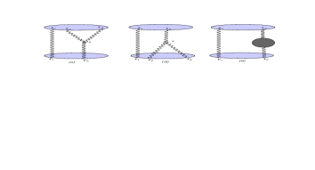
Figure 6: The two “IY-diagrams” and the self-energy correction.

and on $\mathbf{IY}_{\mathbf{down}}$, which is obtained from $\mathbf{IY}_{\mathbf{up}}$ by exchanging the roles of $\sigma$ and $\tau$ (and therefore $x_{i}$ and $y_{i}$). Here $J$ is the constant defined by the integral

$$J=\int_{0}^{2\pi}d\sigma_{1}(\dot{x}_{i}\circ\dot{y}_{1})D(x_{i}-y_{1}),$$ (47)

where $D(x)$ is the usual Feyman propagator. When we shrink the upper circle to a point, the logarithmic behavior can originate only from $\mathbf{IY}_{\mathbf{up}}$. The contribution $\mathbf{IY}_{\mathbf{down}}$ yields analogous behavior when we shrink the lower circle. However, when evaluating $\mathbf{IY}_{\mathbf{up}}$, we also encounter divergences at coincident points ($\tau_{1}\to\tau_{2}$) in the integration over the upper circuit. This singularity though is compensated by the standard ultraviolet-divergence of the self-energy graph: half of diagram $\mathbf{Budiag}$ cancels the divergence for $\tau_{1}\to\tau_{2}$, while the other half cancels the same singularity in $\mathbf{IY}_{\mathbf{down}}$ for $\sigma_{1}\to\sigma_{2}$. Therefore, in order to safely extract the logarithmic behavior when we shrink the circuit to zero, we have to first realize this cancellation.

To begin with, performing a trivial integration by parts, we can rewrite $\mathbf{IY}_{\mathbf{up}}$ in the following form

$$\begin{split}\mathbf{IY}_{\mathbf{up}}=&\frac{\lambda^{3}J}{8N^{3}}\left[\int^{2\pi}_{0}d\tau_{1}d\tau_{2}d\tau_{3}d\sigma_{2}\varepsilon(\tau_{1},\tau_{2},\tau_{3})\right.\{(\dot{x}_{1}\circ\dot{y}_{2})2\dot{x}_{2}\cdot\partial_{y_{2}}-(\dot{x}_{1}\circ\dot{x}_{2})\dot{y}_{2}\cdot\partial_{x_{2}}\}\mathcal{I}_{1}(x_{1},x_{2},y_{2})+\\ &-2\int^{2\pi}_{0}d\tau_{1}d\tau_{2}d\sigma_{2}(\dot{x}_{1}\circ\dot{y}_{2})\mathcal{I}_{1}(x_{1},x_{2},y_{2})\left.+\frac{1}{2}\int^{2\pi}_{0}d\tau_{1}d\tau_{3}d\sigma_{2}(\dot{x}_{1}\circ\dot{y}_{2})\mathcal{I}_{1}(x_{1},x_{1},y_{2})\right].\end{split}$$ (48)

The singular part for coincident points is now singled out in the last term, which is proportional to $\mathcal{I}_{1}(x_{1},x_{1},y_{2})$. Since

$$\begin{split}\mathbf{Budiag}=-&\frac{\lambda^{3}J}{8N^{2}}\int_{0}^{2\pi}d\tau_{1}d\tau_{3}d\sigma_{2}(\dot{x}_{1}\circ\dot{y}_{2})\mathcal{I}_{1}(x_{1},x_{1},y_{2}).\end{split}$$ (49)

half of $\mathbf{Budiag}$ exactly cancels the singularity present in $\mathbf{Y}_{{\mathbf{up}}}$ and we are left with

$$\begin{split}\mathbf{IY}_{\mathbf{up}}=&\frac{\lambda^{3}J}{8N^{2}}\left[\int^{2\pi}_{0}d\tau_{1}d\tau_{2}d\tau_{3}d\sigma_{2}\varepsilon(\tau_{1},\tau_{2},\tau_{3})\right.\{(\dot{x}_{1}\circ\dot{y}_{2})2\dot{x}_{2}\cdot\partial_{y_{2}}-(\dot{x}_{1}\circ\dot{x}_{2})\dot{y}_{2}\cdot\partial_{x_{2}}\}\mathcal{I}_{1}(x_{1},x_{2},y_{2})-\\ &\left.-2\int^{2\pi}_{0}d\tau_{1}d\tau_{2}d\sigma_{2}(\dot{x}_{1}\circ\dot{y}_{2})\mathcal{I}_{1}(x_{1},x_{2},y_{2})\right].\end{split}$$ (50)

This expression does not exhibit any singularity at coincident points. The logarithmic part arising when we shrink the upper circle to a point is then obtained by replacing $\mathcal{I}_{1}$ in the above expression with the $\mathcal{I}_{1}^{sing.}$ found in appendix A. Next we Taylor-expand in $r$ and integrate over the circuits. At leading order in $r$ we find

$$\mathbf{IY}_{\mathbf{up}}^{\mathbf{sing.}}=-\frac{r^{4}\cos^{4}\left(\frac{\theta_{2}}{2}\right)\log(r)}{256\pi^{2}}+O(r^{5})$$ (51)

Let us now sum all the different contributions at leading order in $r$

$$\mathbf{X}^{\mathbf{sing.}}+\mathbf{IY}_{up}^{\mathbf{sing.}}+\mathbf{A_{1}}^{\mathbf{sing.}}+\mathbf{A_{2}}^{\mathbf{sing.}}=\frac{r^{4}\cos^{4}\left(\frac{\theta_{2}}{2}\right)\log(r)}{\pi^{2}}\left(\frac{5}{768}-\frac{1}{256}+\frac{1}{512}-\frac{7}{1536}\right)=0\ !$$ (52)

Namely, we have verified that the logarithmic singularities cancel at the first non trivial order. This implies that the effective anomalous dimension of the operator $\mathcal{O}_{\cal F}$ defined in the previous section vanishes at one-loop, supporting the idea that this operator is actually protected.

As we will show in the next section, this result is consistent with the result coming from the zero instanton expansion of QCD₂.

4 The conjectured matrix model description

In the previous sections we have tried to argue that the correlator of two (or more) Wilson-loops of type (1) might be an exactly solvable quantity since it belongs to a topological sector of $\mathcal{N}=4$. This idea, in fact, passes a certain number of non trivial tests: [a] the observable is $1/8$ BPS independently of the position and the form of the loops [5]; [b] there is a candidate topological twist of the $\mathcal{N}=4$ theory, where one of the supercharges preserving the correlator becomes a scalar [5]; [c] finally, if we compute the behavior of the correlator when one of the circuits shrinks to a point we get a smooth limit with no logarithmic singularity. This last property in particular, should be contrasted with what happens for the correlator of two circular Maldacena-Wilson loops [19]: there the logarithmically singular behavior was present and signaled the impossibility of a matrix model description for this observable [19].

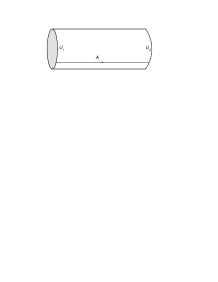
Figure 7: Cylinder amplitude

In this section we shall accept this idea, and focus our attention on the problem of writing a general formula for the correlator of two Wilson-loops. The starting point is to recall that the expectation value of one Wilson-loop appears to be computed by the matrix model describing the zero-instanton sector of a Wilson loop for $QCD_{2}$ on the two sphere [5, 10, 11]. Since the single Wilson loop and the correlator generically share the same symmetries we expect that this equivalence also extends to the case of correlators. Therefore we conjecture that the correlator of two Wilson loops of type (1) is given by the multi-matrix model, which evaluates the zero-instanton sector of the correlator of two loops for $QCD_{2}$ on $S^{2}$.

The construction of this matrix model is quite simple since $QCD_{2}$ is an almost topological theory (it is invariant under area-preserving diffeomorphisms) and its observables can be computed with the help of some simple string-like Feynman-rules [26]. For the present computation we need just three ingredients: the cylinder amplitude (heat-kernel propagator), the disc and the Feynman rule for the observable, i.e. the Wilson loop. The first quantity is represented in fig. 7 and is given by

$$\mathcal{K}(A;U_{1},U_{2})=\langle U_{2}|e^{-\frac{g^{2}A\triangle}{2}}|U_{1}\rangle=\sum_{R}\chi_{R}(U_{1})\chi^{\dagger}_{R}(U_{2})e^{-\frac{g^{2}A}{2}C_{2}(R)},$$ (53)

where $A$ is the area of the cylinder and the sum runs over all the representations $R$ of $U(N)$. The amplitude also depends on the two holonomies $U_{1}$ and $U_{2}$ defined on the two borders of the cylinder. There is in fact a dual representation for the cylinder amplitude where the sum over representations is replaced with a sum over the instanton charges

$$\mathcal{K}(A;U_{1},U_{2})=\!\sum_{P\in S_{N}}\frac{(g^{2}A)^{-N/2}}{J(\theta_{i})J(\phi_{i})}\sum_{\mathbf{\ell}\in\mathds{Z}^{N}}(-1)^{P+(N-1)\sum\ell_{i}}\exp\left({-\frac{1}{2g^{2}A}\sum_{i=1}^{N}(\phi_{i}-\theta_{P(i)}+2\pi i\ell_{i})^{2}}\right),$$ (54)

where $\{e^{i\theta_{i}}\}$ and $\{e^{i\phi_{i}}\}$ are the eigenvalues of the matrices $U_{1}$ and $U_{2}$ respectively and

$$J(\theta_{i})=\prod_{i\leq j}2\sin\left(\frac{\theta_{i}-\theta_{j}}{2}\right).$$

The disc is obtained from (53) by choosing one of the two holonomies to be trivial - namely equal to the identity. Finally, the insertion of a Wilson loop with winding number $n$ is realized by introducing the factor $\mathrm{Tr}(U^{n})$ at the border of the cylinder. The amplitude for the correlator of two non-intersecting loops with winding numbers $n_{1}$ and $n_{2}$ is schematically represented in fig. 8, and the corresponding expression is given by the following two-matrix integral over the unitary matrices:

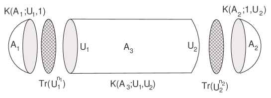
Figure 8: The string-like Feynman-diagram for the correlator of two Wilson-loops.

$$\!\!\!\!\!\begin{split}\tilde{\mathcal{W}}(A_{1},A_{2})=&\frac{1}{N^{2}}\!\int\!\!\mathcal{D}U_{1}\mathcal{D}U_{2}\text{Tr}(U_{1}^{n_{1}})\text{Tr}(U_{2}^{n_{2}})\mathcal{K}(A_{1};\mathds{1},U_{1})\mathcal{K}(A_{3};U_{1},U_{2})\mathcal{K}(A_{2};U_{2},\mathds{1})=\\ =&\frac{1}{N^{2}}\sum_{P\in S_{N}}\sum_{\ell,m,s\in\mathds{Z^{N}}}\int d^{N}\theta d^{N}\phi J^{2}(\theta_{i})J^{2}(\phi_{i})\left(\sum_{r,s=1}^{N}e^{in_{1}\theta_{r}+in_{2}\phi_{s}}\right)\times\\ &\times\frac{(g^{2}A_{1})^{-\frac{N^{2}}{2}}}{J(\theta_{i})}(-1)^{(N-1)\sum_{i}\ell_{i}}\Delta(\theta_{i}+2\pi\ell_{i})\exp\left(-\frac{1}{2g^{2}A_{1}}\sum_{i=1}^{N}(\theta_{i}+2\pi\ell_{i})^{2}\right)\times\\ &\times\!\frac{(g^{2}A_{3})^{-N/2}}{J(\theta_{i})J(\phi_{i})}(-1)^{P+(N-1)\sum s_{i}}\exp\left({-\frac{1}{2g^{2}A_{3}}\sum_{i=1}^{N}(\phi_{i}-\theta_{P(i)}+2\pi is_{i})^{2}}\right)\\ &\times\frac{(g^{2}A_{2})^{-\frac{N^{2}}{2}}}{J(\phi_{i})}(-1)^{(N-1)\sum_{j}m_{j}}\Delta(\phi_{j}+2\pi m_{j})\exp\left(-\frac{1}{2g^{2}A_{2}}\sum_{i=1}^{N}(\phi_{i}+2\pi m_{i})^{2}\right),\end{split}$$ (55)

$\Delta$ being the Vandermonde determinant. The amplitude $\tilde{\mathcal{W}}(A_{1},A_{2})$ is related to the true correlator by the relation $\tilde{\mathcal{W}}(A_{1},A_{2})=\mathcal{Z}\mathcal{W}(A_{1},A_{2})$, where $\mathcal{Z}$ is the partition function of $QCD_{2}$ on the sphere. We can extend the region of integration over the entire $\mathds{R}^{2N}$ by means of the sum over $\ell$ and $m$ and we can rewrite the above expression as

$$\begin{split}&\tilde{\mathcal{W}}(A_{1},A_{2})=\frac{(g^{4}A_{1}A_{2})^{-\frac{N^{2}}{2}}(g^{2}A_{3})^{-\frac{N}{2}}}{N^{2}}\sum_{P\in S_{N}}\sum_{s\in\mathds{Z^{N}}}(-1)^{P+(N-1)\sum s_{i}}\!\!\!\int_{\mathds{R}^{2N}}\!\!\!\!\!\!\!d^{N}\theta d^{N}\phi\left(\sum_{r,s=1}^{N}e^{in_{1}\theta_{r}+in_{2}\phi_{s}}\right)\!\!\times\\ &\times\Delta(\theta_{i})\Delta(\phi_{i})\exp\left(-\frac{1}{2g^{2}A_{1}}\sum_{i=1}^{N}\theta_{i}^{2}-\frac{1}{2g^{2}A_{3}}\sum_{i=1}^{N}(\phi_{i}-\theta_{P(i)}+2\pi is_{i})^{2}-\frac{1}{2g^{2}A_{2}}\sum_{i=1}^{N}\phi_{i}^{2}\right).\end{split}$$ (56)

The result (56) is the exact amplitude and it contains all instantonic corrections. To single out the zero-instanton sector of this amplitude it is sufficient to consider the case where all instanton numbers $s_{i}$ vanish. If we introduce the diagonal matrices $\Theta=\mathrm{diag}(\theta_{1},\dots,\theta_{N})$ and $\Phi=\mathrm{diag}(\phi_{1},\dots,\phi_{N})$, using the Itzykson-Zuber integration formula and defining the hermitian matrices $V_{1}=U^{-1}\Theta U$ and $V_{2}=V\Phi V^{-1}$, we can recast the original integral as the following hermitian two matrix model for the correlator of two Wilson loops

$$W(A_{1},A_{2})= \frac{1}{C_{N}N^{2}}\int DV_{1}DV_{2}{\rm e}^{-\frac{A_{1}+A_{3}}{2g^{2}A_{1}A_{3}}\mathrm{Tr}(V_{1}^{2})-\frac{A_{2}+A_{3}}{2g^{2}A_{2}A_{3}}\mathrm{Tr}(V_{2}^{2})+\frac{1}{g^{2}A_{3}}\mathrm{Tr}(V_{1}V_{2})}\mathrm{Tr}(e^{in_{1}V_{1}})\mathrm{Tr}(e^{in_{2}V_{2}})=$$

$$= \frac{1}{C_{N}N^{2}}\int DV_{1}DV_{2}{\rm e}^{-\frac{1}{2g^{2}A_{1}}\mathrm{Tr}(V_{1}^{2})-\frac{1}{2g^{2}A_{2}}\mathrm{Tr}(V_{2}^{2})-\frac{1}{2g^{2}A_{3}}\mathrm{Tr}((V_{1}-V_{2})^{2})}\mathrm{Tr}(e^{in_{1}V_{1}})\mathrm{Tr}(e^{in_{2}V_{2}}),$$ (57)

where the normalization is chosen to be

$$C_{N}=\int DV_{1}DV_{2}{\rm e}^{-\frac{A_{1}+A_{3}}{2g^{2}A_{1}A_{3}}\mathrm{Tr}(V_{1}^{2})-\frac{A_{2}+A_{3}}{2g^{2}A_{2}A_{3}}\mathrm{Tr}(V_{2}^{2})+\frac{1}{g^{2}A_{3}}\mathrm{Tr}(V_{1}V_{2})}.$$ (58)

Actually, in the sector $s_{i}=0$ of (56), the angular integration can be performed by means of an expansion in terms of Hermite polynomials and by exploiting the relation between integrals over Hermite polynomials and Laguerre polynomials. Then one finds the following finite $N$ closed expression for the connected correlator

$$W(A_{1},A_{2})-W(A_{1})W(A_{2})=$$

$$= \frac{1}{N^{2}}e^{-\frac{\left(A_{1}A_{2}(n_{1}+n_{2})^{2}+A_{3}(n^{2}_{1}A_{1}+n_{2}^{2}A_{2})\right)g^{2}}{2A}}L^{1}_{N-1}\left({\frac{g^{2}\left(A_{3}n_{1}+A_{2}(n_{1}+n_{2})\right)\left(A_{1}(n_{1}+n_{2})+A_{3}n_{2}\right)}{A}}\right)+$$

$$-\frac{1}{N^{2}}e^{-\frac{\left(A_{1}\left(A_{2}+A_{3}\right)n_{1}^{2}+A_{2}\left(A_{1}+A_{3}\right)n_{2}^{2}\right)g^{2}}{2A}}\times$$ (59)

$$\times\sum_{i_{1},i_{2}=1}^{N}\left(-\frac{g^{2}n_{1}n_{2}A_{1}A_{2}}{A}\right)^{i_{2}-i_{1}}\frac{(i_{1}-1)!}{(i_{2}-1)!}L_{i_{1}-1}^{i_{2}-i_{1}}\left({\frac{g^{2}n_{2}^{2}A_{2}(A_{3}+A_{1})}{A}}\right)L^{i_{2}-i_{1}}_{i_{1}-1}\left({\frac{g^{2}n_{1}^{2}A_{1}(A_{3}+A_{2})}{A}}\right)\!\!,$$

where $A=A_{1}+A_{2}+A_{3}$ is the total area of the sphere. For small $g$ this expression can be expanded in a power series and one finds

$$\begin{split}W(A_{1},A_{2})&-W(A_{1})W(A_{2})=-\frac{{A_{1}}{A_{2}}g^{2}n_{1}n_{2}}{NA}+\\ &+\frac{{A_{1}}{A_{2}}({A_{1}}{A_{2}}(n_{1}^{2}+n_{2}^{2}+n_{1}n_{2})+{A_{3}}({A_{1}}n_{1}^{2}+{A_{2}}n_{2}^{2}))g^{4}n_{1}n_{2}}{2A^{2}}+\\ &-g^{6}n_{1}{n_{2}}\left(\frac{{A_{1}}^{3}{A_{2}}({A_{2}}+{A_{3}})^{2}\left(2N^{3}+N\right)n_{1}^{4}}{24A^{3}N^{2}}+\frac{{A_{1}}^{3}{A_{2}}^{2}({A_{2}}+{A_{3}})\left(2N^{3}+N\right){n_{2}}n_{1}^{3}}{12A^{3}N^{2}}+\right.\\ &+\left.\frac{{A_{1}}^{2}{A_{2}}^{2}\left(3{A_{3}}({A_{2}}+{A_{3}})N^{2}+{A_{1}}\left(3{A_{3}}N^{2}+{A_{2}}\left(4N^{2}+1\right)\right)\right){n_{2}}^{2}n_{1}^{2}}{12A^{3}N}+\right.\\ &+\frac{{A_{1}}^{2}{A_{2}}^{3}({A_{1}}+{A_{3}})\left(2N^{3}+N\right){n_{2}}^{3}n_{1}}{12A^{3}N^{2}}+\left.\frac{{A_{1}}{A_{2}}^{3}({A_{1}}+{A_{3}})^{2}\left(2N^{3}+N\right){n_{2}}^{4}}{24A^{3}N^{2}}\right)+O(g^{7}).\end{split}$$ (60)

This result, after decompactifying the sphere, agrees with the perturbative results we have obtained up to ${\cal O}(g^{6})$ from Feynman graph calculations using the Mandelstam-Leibbrandt prescription for the vector propagator in light-cone coordinates [18]. Let us compare the perturbative result (60) with the actual computation in $\mathcal{N}=4$ done in section 3. After performing the standard redefinition $g^{2}\mapsto-g^{2}/A$ and setting $n_{1}=n_{2}=1$, we find complete agreement up to order $g^{4}$. Notice, moreover, that the agreement with $QCD_{2}$ demands the absence of logarithmic singularities when the area of one of the loops is small, to all orders in perturbation theory. Our $g^{6}$ result of sec. 3 is consistent with this prediction.

In order to analyse the large $N$ limit, we can write a simple compact representation for the connected correlator in $\mathcal{N}=4$ SYM by exploiting a contour representation of the Laguerre polynomials

$$W(A_{1},A_{2})-W(A_{1})W(A_{2})=\frac{n_{1}n_{2}}{N^{2}}\int_{C_{1}}\frac{dw_{1}}{2\pi i}\int_{C_{2}}\frac{dw_{2}}{2\pi i}\frac{e^{w_{1}+w_{2}+\frac{\lambda\left(\tilde{A_{1}}A_{1}w_{2}n_{1}^{2}+\tilde{A_{2}}A_{2}n_{2}^{2}w_{1}\right)}{A^{2}w_{2}w_{1}}}\tilde{A_{2}}A_{1}}{\left(\tilde{A_{2}}n_{2}w_{1}-A_{1}n_{1}w_{2}\right)^{2}},$$ (61)

where $\tilde{A}_{1}=A-A_{1}$ and $\tilde{A}_{2}=A-A_{2}$. This expression can be computed as an infinite series of Bessel functions. We limit our attention to the case $n_{1}=n_{2}=1$ and are actually interested in the normalized correlator, which is given by

$$\frac{W_{conn.}}{W_{1}W_{2}}=\frac{\lambda}{N^{2}A^{2}}\tilde{A}_{1}\tilde{A}_{2}\sum_{k=1}^{\infty}k\left(\sqrt{\frac{A_{1}A_{2}}{\tilde{A}_{1}\tilde{A}_{2}}}\right)^{k+1}\frac{I_{k}\left(2{\sqrt{\frac{\lambda A_{2}\tilde{A}_{2}}{A^{2}}{}}}\right)}{I_{1}\left(2{\sqrt{\frac{\lambda A_{2}\tilde{A}_{2}}{A^{2}}{}}}\right)}\frac{I_{k}\left(2{\sqrt{\frac{\lambda A_{1}\tilde{A}_{1}}{A^{2}}}}\right)}{I_{1}\left(2{\sqrt{\frac{\lambda A_{1}\tilde{A}_{1}}{A^{2}}{}}}\right)}.$$ (62)

In the next section we will be interested in comparing this result with the strong coupling prediction of super-gravity. For this reason, we have to expand the above result for large $\lambda$. This can easily be done by recalling that

$$\frac{I_{k}\left(z\right)}{I_{1}\left(z\right)}=1+O\left(\frac{1}{z}\right).$$ (63)

Then the correlator in the strong coupling regime becomes

$$\frac{W_{conn.}}{W_{1}W_{2}}\sim\frac{\lambda}{N^{2}}\frac{\tilde{A}_{1}\tilde{A}_{2}}{A^{2}}\left[\frac{A_{1}A_{2}}{\tilde{A}_{1}\tilde{A}_{2}}+2\left(\sqrt{\frac{A_{1}A_{2}}{\tilde{A}_{1}\tilde{A}_{2}}}\right)^{3}+\cdots\right].$$ (64)

The first term in the expansion corresponds to the $U(1)$ factor present in $U(N)$ and we shall drop it since it is not generally considered in the super-gravity analysis. The first non trivial term which can be compared with super-gravity is the second one.

5 Correlator at strong coupling

We can also use the AdS/CFT correspondence [28] to compute the correlator of the latitudes at strong coupling, in the limit where they are well separated compared to their radii, i.e. in the limit that they migrate to opposite poles of the sphere. In this limit the correlator is dominated by the exchange of light SUGRA modes between the two worldsheets describing the Wilson loops at strong coupling [21, 29, 30, 27].

Sometimes, as has been the case for certain chiral primary operators, two point functions with the Wilson loop can be computed exactly [29, 27] in the gauge theory and succesfully compared at strong coupling to a SUGRA calculation of the same quantity. Indeed, by taking the “square-root” of the contribution to the correlator of two Wilson loops from a specific SUGRA mode, the two-point function of the Wilson loop with the operator dual to that mode is recovered [21]. In this section we will present a striking agreement between the exchange of certain such SUGRA modes and the strong-coupling limit of the QCD₂ result (62). In order to prove that the QCD₂ result truly captures the correlator at strong coupling, cancellations between further SUGRA modes will have to be demonstrated. We leave this to a further publication [18].

5.1 An intriguing connection

There appears to be a rather intimate connection between the QCD₂ result presented in section 4 and the two-point functions of latitude Wilson loops with chiral primary operators built upon the scalar field $\Phi_{3}$. In the work [27] it was shown that

$$\frac{\langle W\,\widetilde{O}_{J}(x)\rangle}{\langle W\rangle}=\frac{1}{2N}\left(\frac{R\sin\theta}{x^{2}}\right)^{J}\sqrt{J\lambda}\sin\theta\frac{I_{J}\left(\sqrt{\lambda}\,\sin\theta\right)}{I_{1}\left(\sqrt{\lambda}\sin\theta\right)},$$ (65)

where $W$ is a latitude Wilson loop at polar angle $\theta$ and

$$\widetilde{O}_{J}(x)=\frac{1}{\sqrt{J\lambda}}\text{Tr}\,\left(\Phi_{3}+i\Phi_{4}\right)^{J},$$ (66)

where $x\gg R\sin\theta$ measures the perpendicular distance between the operator and the loop. This demonstrates that the matrix model which yields (2) also captures two-point functions with those CPO’s sharing a minimum amount of SUSY with the latitude Wilson loop.

Let us look then at the contribution of the $\widetilde{O}_{J}$ to the correlator of two latitudes, at polar angles $\theta_{0}$ and $\theta_{1}$, taken near opposite poles of the sphere to enforce $x\gg R\sin\theta$. Note that $x=R\cos\theta_{0}-R\cos\theta_{1}$, we then have

$$\begin{split}\frac{\langle W_{0}\,W_{1}\rangle}{\langle W_{0}\rangle\langle W_{1}\rangle}\Biggr{|}_{\widetilde{O}_{J}}=\frac{\lambda\sin\theta_{0}\sin\theta_{1}}{4N^{2}}\sum_{J=2}^{\infty}\,J\,&\left(\frac{\sin\theta_{0}\,\sin\theta_{1}}{(\cos\theta_{0}-\cos\theta_{1})^{2}}\right)^{J}\\ &\times\frac{I_{J}\left(\sqrt{\lambda}\,\sin\theta_{0}\right)}{I_{1}\left(\sqrt{\lambda}\sin\theta_{0}\right)}\frac{I_{J}\left(\sqrt{\lambda}\,\sin\theta_{1}\right)}{I_{1}\left(\sqrt{\lambda}\sin\theta_{1}\right)}.\end{split}$$ (67)

This expression is valid strictly at leading order in the large separation limit. The reason for this is that (67) ignores quantum corrections between the propagators joining the operator to the Wilson loop; this is only valid in the strict large separation limit as shown in [23, 27]. The expression (67) bears a striking resemblance to the QCD₂ result (62). In fact, the only difference lies in the factor in round parentheses which is risen to the power $J$. However, taking the large-separation limit of this factor, that difference disappears and (67) is exactly equal to (62). Thus the QCD₂ result gives, in the large-separation limit, exactly the contribution of the exchange of (66). This agreement is valid at any value of the coupling, and indeed, in [27] it was shown that at strong coupling the result is recovered from supergravity.

At leading order in weak coupling, this agreement is puzzling for the following reason. It is not exactly the operator (66) which is present in the latitudes’ OPE, since there is no coupling to $\Phi_{4}$. Indeed, the calculation of the correlator given in (14) shows that all the operators present in the latitude’s OPE (12) participate in the correlator at this order in $\lambda$. It is therefore a curious coincidence that (66) produces the same contribution at weak coupling (i.e. $J=2$) as the true composite operator (12) present in the actual OPE. Before addressing this issue further, we present a remarkable strong coupling calculation.

It is interesting to go beyond the strict large-separation limit, and test the QCD₂ result (62) to higher orders in the shrinking radii of the two latitudes. It turns out that at strong coupling, the associated SUGRA calculation giving this information is tractable. In keeping with the intriguing connection between the contribution of (66) to the correlator and the QCD₂ result, we begin by computing the exchange of the SUGRA modes dual to (66) in an expansion about small latitude radii $\theta_{0}$ and $\theta_{1}$ (where the polar angle of the latitude at the south pole is given by $\pi-\theta_{1}$).

The supergravity modes dual to (66) are fluctuations of the RR 5-form as well as the spacetime metric. They are by now very well known, and details can be found in [21][22][32][29][30]. The fluctuations of the metric are

$$\delta g_{\mu\nu} = \left[-\frac{6\,J}{5}\,g_{\mu\nu}+\frac{4}{J+1}\,D_{(\mu}D_{\nu)}\right]\,s^{J}(x)\,Y^{J}(\Omega),$$ (68)

$$\delta g_{\alpha\beta} = 2\,J\,g_{\alpha\beta}\,s^{J}(x)\,Y_{J}(\Omega),$$ (69)

where $\mu,\nu$ are $AdS_{5}$ and $\alpha,\beta$ are $S^{5}$ indices. The symbol $x$ indicates coordinates on $AdS_{5}$ and $\Omega$ coordinates on the $S^{5}$. The bulk-to-bulk scalar propagator for the field $s^{J}(x)$ is

$$P(x,\bar{x})=\frac{\alpha_{0}}{B_{J}}\,W^{J}\,{{}_{2}}F_{1}(\,J,\,J-3/2,\,2J-3;\,-4W)$$ (70)

where in an $AdS_{5}$ given by $ds^{2}=(dx_{0}^{2}+dx_{i}^{2})/x_{0}^{2}$, $W=x_{0}\bar{x}_{0}/((x_{0}-\bar{x}_{0})^{2}+(x_{i}-\bar{x}_{i})^{2})$. The full details of the calculation will be presented in [18], however it is essentially that found in [27]. There, the strict large-separation limit was employed by setting the hypergeometric function to 1. Here we keep higher terms in the expansion. The results are as follows

$$\begin{split}&J=2~{}:\qquad\frac{\langle W(x)\,W(\bar{x})\rangle}{\langle W(x)\rangle\langle W(\bar{x})\rangle}=\frac{\lambda}{8N^{2}}\Biggl{[}\frac{\theta_{0}^{3}\,\theta_{1}^{3}}{2^{2}}+\frac{\theta_{0}^{3}\,\theta_{1}^{7}+\theta_{0}^{7}\,\theta_{1}^{3}}{5\cdot 3\cdot 2^{6}}+\frac{\theta_{0}^{5}\,\theta_{1}^{5}}{2^{6}}+\frac{\theta_{0}^{3}\,\theta_{1}^{9}+\theta_{0}^{9}\,\theta_{1}^{3}}{7\cdot 3^{3}\cdot 2^{6}}\\ &\qquad\qquad\qquad\qquad\qquad\qquad\qquad\qquad+\frac{\theta_{0}^{5}\,\theta_{1}^{7}+\theta_{0}^{7}\,\theta_{1}^{5}}{3\cdot 2^{7}}+\frac{\theta_{0}^{6}\,\theta_{1}^{6}}{5^{2}\cdot 3}-\frac{\theta_{0}^{7}\,\theta_{1}^{6}+\theta_{0}^{6}\,\theta_{1}^{7}}{5\cdot 3\cdot 2^{3}}+{\cal O}(\theta^{14})\Biggr{]},\\ &J=3~{}:\qquad\frac{\langle W(x)\,W(\bar{x})\rangle}{\langle W(x)\rangle\langle W(\bar{x})\rangle}=\frac{\lambda}{32N^{2}}\Biggl{[}\frac{3\,\theta_{0}^{4}\,\theta_{1}^{4}}{8}+\frac{\theta_{0}^{4}\,\theta_{1}^{6}+\theta_{0}^{6}\,\theta_{1}^{4}}{2^{5}}+\frac{3\,(\theta_{0}^{4}\,\theta_{1}^{8}+\theta_{0}^{8}\,\theta_{1}^{4})}{5\cdot 2^{7}}\\ &\quad+\frac{5\,\theta_{0}^{6}\,\theta_{1}^{6}}{3\cdot 2^{6}}+\frac{3^{3}\,\theta_{0}^{7}\,\theta_{1}^{7}}{7^{2}\cdot 5^{2}}+\frac{(\theta_{0}^{6}\,\theta_{1}^{8}+\theta_{0}^{8}\,\theta_{1}^{6})}{5\cdot 2^{5}}+\frac{23\,(\theta_{0}^{4}\,\theta_{1}^{10}+\theta_{0}^{10}\,\theta_{1}^{4})}{7\cdot 5\cdot 3^{3}\cdot 2^{7}}-\frac{3^{2}\,(\theta_{0}^{7}\,\theta_{1}^{8}+\theta_{0}^{8}\,\theta_{1}^{7})}{7\cdot 5\cdot 2^{5}}+{\cal O}(\theta^{16})\Biggr{]},\\ &J=4~{}:\qquad\frac{\langle W(x)\,W(\bar{x})\rangle}{\langle W(x)\rangle\langle W(\bar{x})\rangle}=\frac{\lambda}{256N^{2}}\Biggl{[}\theta_{0}^{5}\,\theta_{1}^{5}+\frac{\theta_{0}^{5}\,\theta_{1}^{7}+\theta_{0}^{7}\,\theta_{1}^{5}}{3\cdot 2}+\frac{\theta_{0}^{5}\,\theta_{1}^{9}+\theta_{0}^{9}\,\theta_{1}^{5}}{3^{2}\cdot 2^{2}}+\frac{13\,\theta_{0}^{7}\,\theta_{1}^{7}}{3^{2}\cdot 2^{4}}\\ &\qquad\qquad\qquad\qquad\qquad\qquad\qquad\qquad+{\cal O}(\theta^{16})\Biggr{]}.\end{split}$$ (71)

The QCD₂ result (62) in the large $\lambda$ limit is

$$\frac{\langle W(x)\,W(\bar{x})\rangle}{\langle W(x)\rangle\langle W(\bar{x})\rangle}\Biggr{|}_{QCD_{2}}=\frac{\lambda\sin\theta_{0}\,\sin\theta_{1}}{4N^{2}}\sum_{J=1}^{\infty}J\,\tan^{J}\frac{\theta_{0}}{2}\,\tan^{J}\frac{\theta_{1}}{2}.$$ (72)

Ignoring $J=1$, we may expand in $\theta$ order-by-order in $J$:

$$\begin{split}&J=2~{}:\qquad\frac{\langle W(x)\,W(\bar{x})\rangle}{\langle W(x)\rangle\langle W(\bar{x})\rangle}\Biggr{|}_{QCD_{2}}=\frac{\lambda}{8N^{2}}\Biggl{[}\frac{\theta_{0}^{3}\,\theta_{1}^{3}}{2^{2}}+\frac{\theta_{0}^{3}\,\theta_{1}^{7}+\theta_{0}^{7}\,\theta_{1}^{3}}{5\cdot 3\cdot 2^{6}}+\frac{\theta_{0}^{3}\,\theta_{1}^{9}+\theta_{0}^{9}\,\theta_{1}^{3}}{7\cdot 3^{3}\cdot 2^{6}}+{\cal O}(\theta^{14})\Biggr{]},\\ &J=3~{}:\qquad\frac{\langle W(x)\,W(\bar{x})\rangle}{\langle W(x)\rangle\langle W(\bar{x})\rangle}\Biggr{|}_{QCD_{2}}=\frac{\lambda}{32N^{2}}\Biggl{[}\frac{3\,\theta_{0}^{4}\,\theta_{1}^{4}}{8}+\frac{\theta_{0}^{4}\,\theta_{1}^{6}+\theta_{0}^{6}\,\theta_{1}^{4}}{2^{5}}+\frac{3\,(\theta_{0}^{4}\,\theta_{1}^{8}+\theta_{0}^{8}\,\theta_{1}^{4})}{5\cdot 2^{7}}\\ &\qquad\qquad\qquad\qquad\qquad\qquad+\frac{\theta_{0}^{6}\,\theta_{1}^{6}}{3\cdot 2^{7}}+\frac{(\theta_{0}^{6}\,\theta_{1}^{8}+\theta_{0}^{8}\,\theta_{1}^{6})}{5\cdot 2^{9}}+\frac{23\,(\theta_{0}^{4}\,\theta_{1}^{10}+\theta_{0}^{10}\,\theta_{1}^{4})}{7\cdot 5\cdot 3^{3}\cdot 2^{7}}+{\cal O}(\theta^{16})\Biggr{]},\\ &J=4~{}:\qquad\frac{\langle W(x)\,W(\bar{x})\rangle}{\langle W(x)\rangle\langle W(\bar{x})\rangle}\Biggr{|}_{QCD_{2}}=\frac{\lambda}{256N^{2}}\Biggl{[}\theta_{0}^{5}\,\theta_{1}^{5}+\frac{\theta_{0}^{5}\,\theta_{1}^{7}+\theta_{0}^{7}\,\theta_{1}^{5}}{3\cdot 2}+\frac{\theta_{0}^{5}\,\theta_{1}^{9}+\theta_{0}^{9}\,\theta_{1}^{5}}{3^{2}\cdot 2^{2}}+\frac{\theta_{0}^{7}\,\theta_{1}^{7}}{3^{2}\cdot 2^{2}}\\ &\qquad\qquad\qquad\qquad\qquad\qquad\qquad\qquad\qquad\qquad+{\cal O}(\theta^{16})\Biggr{]}.\end{split}$$ (73)

There is a remarkable matching of highly non-trivial terms between these two calculations! The difference between the two calculations sets-in quite late

$$\begin{split}&\left(\text{SUGRA}-\text{QCD}_{2}\right)_{J=2}=\frac{\lambda}{8N^{2}}\Biggl{[}\frac{\theta_{0}^{5}\,\theta_{1}^{5}}{2^{6}}+\frac{\theta_{0}^{5}\,\theta_{1}^{7}+\theta_{0}^{7}\,\theta_{1}^{5}}{3\cdot 2^{7}}+\frac{\theta_{0}^{6}\,\theta_{1}^{6}}{5^{2}\cdot 3}-\frac{\theta_{0}^{7}\,\theta_{1}^{6}+\theta_{0}^{6}\,\theta_{1}^{7}}{5\cdot 3\cdot 2^{3}}+{\cal O}(\theta^{14})\Biggr{]},\\ &\left(\text{SUGRA}-\text{QCD}_{2}\right)_{J=3}\!=\!\frac{\lambda}{32N^{2}}\!\Biggl{[}\frac{3\,\theta_{0}^{6}\,\theta_{1}^{6}}{2^{7}}+\frac{3\,(\theta_{0}^{6}\,\theta_{1}^{8}+\theta_{0}^{8}\,\theta_{1}^{6})}{2^{9}}+\frac{3^{3}\,\theta_{0}^{7}\,\theta_{1}^{7}}{7^{2}\cdot 5^{2}}-\frac{3^{2}\,(\theta_{0}^{7}\,\theta_{1}^{8}+\theta_{0}^{8}\,\theta_{1}^{7})}{7\cdot 5\cdot 2^{5}}\!+\!{\cal O}(\theta^{16})\!\Biggr{]}\!,\\ &\left(\text{SUGRA}-\text{QCD}_{2}\right)_{J=4}=\frac{\lambda}{256N^{2}}\Biggl{[}\frac{\theta_{0}^{7}\,\theta_{1}^{7}}{2^{4}}+{\cal O}(\theta^{16})\Biggr{]}.\\ \end{split}$$ (74)

Although we have considered values of $J$ up to $J=4$, we expect a similar pattern for arbitrary $J$.

5.2 Other modes

The remarkable agreement displayed in the previous section does not prove that the QCD₂ result captures the correlator of the latitudes at strong coupling. Beyond the issue of the discrepancy at order $\theta_{0}^{5}\theta_{1}^{5}$, the catch is that the SUGRA spectrum contains two other modes which couple to the string worldsheets and also produce $\theta_{0}^{3}\theta_{1}^{3}$ terms, thereby potentially spoiling the agreement with the QCD₂ result. These are the Kaluza-Klein modes of the NS-NS B-field of type-IIB supergravity, and have been described in [32], c.f. their equation (2.48) and what follows it. There is a fluctuation of the B-field with both legs in the $S^{5}$ which is described by a scalar of mass-squared $-3$ (corresponding to a gauge theory operator of protected dimension 3) given by

$$\delta B_{\alpha\beta}=a^{k}_{-}(x)\,Y_{[\alpha\beta]}^{k,-}(\Omega),\qquad m_{a^{k}_{-}}^{2}=k^{2}-4,$$ (75)

with $k=1$. There is also the fluctuation of the B-field with both legs in the $AdS_{5}$ portion of the geometry $\delta B_{\mu\nu}$, which has been discussed in [31]. It has the Kaluza-Klein expansion

$$\delta B_{\mu\nu}=a^{k}_{\mu\nu}(x)\,Y^{k}(\Omega),\qquad m_{a^{k}_{\mu\nu}}^{2}=k^{2},$$ (76)

and the leading $k=1$ harmonic corresponds to the following protected dimension 3 operator (where $A,B$ are SU(4) indices)

$$2i\,\Phi^{AB}F^{+}_{\mu\nu}+\bar{\psi}^{A}\sigma_{\mu\nu}\bar{\psi}^{B}.$$ (77)

These contributions must cancel out if the QCD₂ result is to hold. Beyond these modes, there are also fluctuations of the dilaton, massless vector, and massless tensor which provide contributions which lead as $\theta_{0}^{4}\theta_{1}^{4}$ and must therefore also find a way to cancel each other, should the QCD₂ result truly describe the correlator at strong coupling. Indeed this is the reflection at strong coupling of the curiosity of the fact that the operators of classical dimension 3 and 4 contributing to the correlator at weak coupling seem to have the same effect as replacement by (66) (with $J=2$). The full calculation of these SUGRA modes, and the question of whether or not they cancel, will be explored in a companion publication [18].

The matrix model result (2) contains a rescaled coupling constant $\lambda^{\prime}=\lambda\sin^{2}\theta$. The two point function of the latitude with the CPO (66) leads as $\lambda^{\prime}$ but ends-up as $\sqrt{\lambda^{\prime}}$ at strong coupling. This explains why in the OPE the operator $\text{Tr}\,\Phi_{3}^{2}$ is weighted by $\theta^{4}$ but ends-up contributing as $\theta^{3}$ at strong coupling. The first descendent of this operator appearing in the OPE of the latitude is $\text{Tr}\,\Phi_{3}\partial_{3}\Phi_{3}$ and comes with weight $\theta^{6}$, thus one would expect its contribution at strong coupling to be $\theta^{5}$, potentially explaining why the discrepancy between the QCD₂ result and the contribution from CPO’s built on $\Phi_{3}$ sets-in at order $\theta_{0}^{5}\theta_{1}^{5}$.

Appendix A Appendix

The integral $\mathcal{I}_{1}$ defined in (32), for example, was computed in [10] and a useful representation for the final result is

$$\mathcal{I}_{1}(x_{1},x_{2},x_{3})=\frac{1}{64\pi^{4}}\!\!\!\int_{0}^{1}\!\!\!\!d\alpha\frac{1}{({y}-\alpha{x})^{2}}\log\left[\frac{\alpha[({x}-{y})^{2}-{y}^{2}]+{y}^{2}}{\alpha(1-\alpha){x}^{2}}\right],$$ (A.1)

where $x=x_{1}-x_{2}$ and $y=x_{3}-x_{2}$. The only logarithmic behavior in this integral arises when $x_{1}$ and $x_{2}$ approach the same point $x_{0}$ (namely $|x|\to 0$), and is given by

$$\mathcal{I}_{1}^{sing.}=-\frac{1}{64\pi^{4}}\!\!\!\int_{0}^{1}\!\!\!\!d\alpha\frac{1}{({y}-\alpha{x})^{2}}\log{x}^{2}=-\frac{1}{64\pi^{4}}\!\!\!\int_{0}^{1}\!\!\!\!d\alpha\frac{\log(x_{1}-x_{2})^{2}}{({(x_{3}-x_{2})}-\alpha{(x_{1}-x_{2})})^{2}}.$$ (A.2)

Next we consider the integral

$$\mathcal{I}^{(4)}(x_{1},x_{2},x_{3},x_{4})=\frac{1}{(4\pi^{2})^{4}}\int\frac{d^{4}z}{(x_{1}-z)^{2}(x_{2}-z)^{2}(y_{1}-z)^{2}(y_{2}-z)^{2}}.$$ (A.3)

It is well-known that this integral can be computed in terms of $\mathcal{I}_{1}$ [34]. In fact if we define

$$\bar{x}_{1}^{\mu}=\frac{(x_{1}-y_{2})^{\mu}}{(x_{1}-y_{2})^{2}},\ \ \ \bar{x}_{2}^{\mu}=\frac{(x_{2}-y_{2})^{\mu}}{(x_{2}-y_{2})^{2}},\ \ \ \ \bar{x}_{3}^{\mu}=\frac{(y_{1}-y_{2})^{\mu}}{(y_{1}-y_{2})^{2}},$$ (A.4)

we find

$$\mathcal{I}^{(4)}(x_{1},x_{2},x_{3},x_{4})=\frac{\bar{x}_{1}^{2}\bar{x}_{2}^{2}\bar{x}_{3}^{2}}{(4\pi^{2})^{4}}\int\frac{d^{4}z}{(\bar{x}_{1}-z)^{2}(\bar{x}_{2}-z)^{2}(\bar{x}_{3}-z)^{2}}=\frac{\bar{x}_{1}^{2}\bar{x}_{2}^{2}\bar{x}_{3}^{2}}{4\pi^{2}}\mathcal{I}_{1}(\bar{x}_{1}-\bar{x}_{2},{\bar{x}_{3}}-\bar{x}_{2}).$$ (A.5)

Then

$$\mathcal{I}^{(4)sing.}(x_{1},x_{2},y_{1},y_{2})=-\frac{{\log(x_{1}-x_{2})^{2}}}{256\pi^{6}}\times$$

$$\times\!\int_{0}^{1}\!\!\frac{d\alpha}{\mbox{\small$(1-\alpha){(y_{1}-x_{2})^{2}(y_{2}-x_{1})^{2}}-\alpha(1-\alpha){(x_{1}-x_{2})^{2}(y_{1}-y_{2})^{2}}+{\alpha(y_{1}-x_{1})^{2}(y_{2}-x_{2})^{2}}$}}.$$ (A.6)

For our goals, the most convenient way to compute the integral $\mathcal{S}^{\mu}$ defined in (44) is to use the technique of [35], which allows us to reduce the tensor integrals to scalar integrals in higher space-time dimensions. We shall perform this reduction in $2\omega$ dimensions and for arbitrary powers of the denominators. The final result is very nice and compact

$$\prod_{i=1}^{4}\frac{\Gamma(a_{i})}{4\pi^{a_{i}+1}}\int\frac{w^{\mu}d^{2\omega}w}{((x_{1}-w)^{2})^{a_{1}}((x_{2}-w)^{2})^{a_{2}}((x_{3}-w)^{2})^{a_{3}}((x_{4}-w)^{2})^{a_{4}}}=\sum_{j=1}^{4}x_{j}^{\mu}\mathfrak{S}(\omega+1;a_{i}+\delta_{ij})$$ (A.7)

where

$$\mathfrak{S}^{(2\omega)}(\omega;a_{i})=\prod_{i=1}^{4}\frac{\Gamma(a_{i})}{4\pi^{a_{i}+1}}\int\frac{d^{2\omega}w}{((x_{1}-w)^{2})^{a_{1}}((x_{2}-w)^{2})^{a_{2}}((x_{3}-w)^{2})^{a_{3}}((x_{4}-w)^{2})^{a_{4}}}.$$ (A.8)

In computing $\mathbf{A_{1}}$ we also need the derivative with respect to $x_{2}^{\nu}$ of the above expression. After some manipulation this derivative can be arranged as follows

$$\begin{split}&\prod_{i=1}^{4}\frac{\Gamma(a_{i})}{4\pi^{a_{i}+1}}\frac{\partial}{\partial x_{2}^{\nu}}\int\frac{w^{\mu}d^{2\omega}w}{((x_{1}-w)^{2})^{a_{1}}((x_{2}-w)^{2})^{a_{2}}((x_{3}-w)^{2})^{a_{3}}((x_{4}-w)^{2})^{a_{4}}}=\\ &=\delta^{\mu\nu}\mathfrak{S}(\omega+1;a_{i}+\delta_{i2})+2\pi\sum_{k=1}^{4}\sum_{j=1}^{4}x_{j}^{\mu}(x_{k}-x_{2})^{\nu}\mathfrak{S}(\omega+2;a_{i}+\delta_{ij}+\delta_{i2}+\delta_{ki}).\end{split}$$ (A.9)

Finally, the only other ingredient necessary for our calculation is the behavior of the integral $\mathcal{S}(2\omega;a_{i})$ when $x_{1}$ and $x_{2}$ approach the same point $x_{0}$.

$$\begin{split}\mathcal{S}(2\omega;a_{i})=&\frac{}{}\frac{\Gamma\left(\omega-a_{1}\right)\Gamma\left(\omega-a_{2}\right)\Gamma(a_{3})\Gamma(a_{4})\Gamma\left(a_{1}+a_{2}-\omega\right)}{256\pi^{\mbox{\tiny$\displaystyle{\sum_{i=1}^{4}}$}a_{i}+4-\omega}\Gamma\left(2\omega-a_{1}-a_{2}\right)}\frac{(({{x}_{1}}-{{x}_{2}})^{2})^{\left(\omega-a_{1}-a_{2}\right)}}{(({x}_{3})^{2})^{a_{3}}(({x}_{4})^{2})^{a_{4}}}\times\\ &\times\left[1+2\left(a_{3}\frac{{x}_{3}}{{x}_{3}^{2}}+a_{4}\frac{{x}_{4}}{{x}_{4}^{2}}\right)\cdot\left(({x}_{2}-x_{0})+\frac{\omega-a_{2}}{2\omega-a_{1}-a_{2}}({x}_{1}-{x}_{2})\right)+O(({x}_{1}-{x}_{2})^{2})\right].\end{split}$$ (A.10)

References

- [1] S. J. Rey and J. T. Yee, Eur. Phys. J. C 22, 379 (2001) [arXiv: hep-th/9803001].
- [2] J. M. Maldacena, Phys. Rev. Lett. 80, 4859 (1998) [arXiv: hep-th/9803002].
- [3] N. Drukker, S. Giombi, R. Ricci and D. Trancanelli, [arXiv: hep-th/0711.3226].
- [4] N. Drukker, S. Giombi, R. Ricci and D. Trancanelli, Phys. Rev. D 76 (2007) 107703 [arXiv: hep-th/0704.2237 ].
- [5] N. Drukker, S. Giombi, R. Ricci and D. Trancanelli, Phys. Rev. D 77 (2008) 047901 [arXiv: hep-th/0707.2699 ].
- [6] J. K. Erickson, G. W. Semenoff and K. Zarembo, Nucl. Phys. B 582 (2000) 155 [arXiv: hep-th/0003055].
- [7] N. Drukker and D. J. Gross, J. Math. Phys. 42, 2896 (2001) [arXiv: hep-th/0010274]
- [8] V. Pestun, [arXiv: hep-th/0712.2824].
- [9] N. Drukker, JHEP 0609 (2006) 004 [arXiv: hep-th/0605151].
- [10] A. Bassetto, L. Griguolo, F. Pucci and D. Seminara, JHEP 0806 (2008) 083 [arXiv: hep-th/0804.3973 ].
- [11] D. Young, JHEP 0805 (2008) 077 [arXiv: hep-th/0804.4098].
- [12] A. Bassetto and L. Griguolo, Phys. Lett. B 443, 325 (1998) [arXiv: hep-th/9806037].
- [13] N. Drukker and J. Plefka, JHEP 0904 (2009) 052 [arXiv: hep-th/0901.3653].
- [14] T. T. Wu, “Two-Dimensional Yang-Mills Theory In The Leading 1/N Expansion,” Phys. Lett. B 71, 142 (1977).
- [15] S. Mandelstam, “Light Cone Superspace And The Ultraviolet Finiteness Of The N=4 Model,” Nucl. Phys. B 213, 149 (1983).
- [16] G. Leibbrandt, “The Light Cone Gauge In Yang-Mills Theory,” Phys. Rev. D 29, 1699 (1984).
- [17] M. Staudacher and W. Krauth, Phys. Rev. D 57, 2456 (1998) [hep-th/9709101].
- [18] A. Bassetto, G. Griguolo, F. Pucci, D. Seminara, S. Thambyahpillai and D. Young to appear
- [19] G. Arutyunov, J. Plefka and M. Staudacher, JHEP 0112, 014 (2001) [arXiv: hep-th/0111290].
- [20] S. Giombi, V. Pestun and R. Ricci, [arXiv: hep-th/0905.0665].
- [21] D. E. Berenstein, R. Corrado, W. Fischler and J. M. Maldacena, Phys. Rev. D 59 (1999) 105023 [arXiv:hep-th/9809188].
- [22] S. Lee, S. Minwalla, M. Rangamani and N. Seiberg, Adv. Theor. Math. Phys. 2 (1998) 697 [arXiv:hep-th/9806074].
- [23] V. Pestun and K. Zarembo, Phys. Rev. D 67 (2003) 086007 [arXiv:hep-th/0212296].
- [24] G. W. Semenoff and K. Zarembo, Nucl. Phys. B 616 (2001) 34 [arXiv:hep-th/0106015].
- [25] N. Beisert, C. Kristjansen, J. Plefka, G. W. Semenoff and M. Staudacher, Nucl. Phys. B 650 (2003) 125 [arXiv:hep-th/0208178].
- [26] E. Witten, J. Geom. Phys. 9, 303 (1992) [arXiv: hep-th/9204083].
- [27] G. W. Semenoff and D. Young, Phys. Lett. B 643, 195 (2006) [arXiv: hep-th/0609158].
- [28] J. M. Maldacena, Adv. Theor. Math. Phys. 2, 231 (1998) [Int. J. Theor. Phys. 38, 1113 (1999)] [arXiv: hep-th/9711200].
- [29] G. W. Semenoff and D. Young, Int. J. Mod. Phys. A 20 (2005) 2833 [arXiv: hep-th/0405288].
- [30] S. Giombi, R. Ricci and D. Trancanelli, JHEP 0610, 045 (2006) [arXiv: hep-th/0608077].
- [31] G. E. Arutyunov and S. A. Frolov, Phys. Lett. B 441 (1998) 173 [arXiv:hep-th/9807046].
- [32] H. J. Kim, L. J. Romans and P. van Nieuwenhuizen, Phys. Rev. D 32 (1985) 389.
- [33] S. Ferrara, C. Fronsdal and A. Zaffaroni, Nucl. Phys. B 532 (1998) 153 [arXiv: hep-th/9802203].
- [34] J. M. Drummond, J. Henn, V. A. Smirnov and E. Sokatchev, JHEP 0701, 064 (2007) [arXiv:hep-th/0607160].
- [35] A. I. Davydychev, Phys. Lett. B 263, 107 (1991).
- [36] S. Giombi and V. Pestun, arXiv:0906.1572 [hep-th].