Integrated Sachs-Wolfe Effect for Gravitational Radiation

Abstract

Gravitational waves are messengers carrying valuable information about their sources. For sources at cosmological distances, the waves will contain also the imprint left by the intervening matter. The situation is in close analogy with cosmic microwave photons, for which the large-scale structures the photons traverse contribute to the observed temperature anisotropies, in a process known as the integrated Sachs-Wolfe effect. We derive the gravitational wave counterpart of this effect for waves propagating on a Friedman-Robertson-Walker background with scalar perturbations. We find that the phase, frequency and amplitude of the gravitational waves experience Sachs-Wolfe type integrated effects, this in addition to the magnification effects on the amplitude from gravitational lensing. We show that for supermassive black hole binaries, the integrated effects could account for measurable changes on the frequency, chirp mass and luminosity distance of the binary, thus unveiling the presence of inhomogeneities, and potentially dark energy, in the Universe.

Observations of gravitational waves (GWs) have a tremendous potential for transforming our understanding of the cosmos. For sources at cosmological distances, such as the inspiral of supermassive black hole (BH) binaries in the sensitivity window of the proposed Laser Interferometer Space Antenna (LISA), GWs will not only carry information of the characteristics of the source but also contain information on the cosmological expansion of space-time through which these waves propagate, yielding redshifted measurements of the properties of the binary (e.g. distance, chirp-mass, frequency) (Hughes and Holz, 2003; Finn, 1996; Flanagan and Hughes, 1998). When combined with a coincident electromagnetic (EM) counterpart, GWs observations from supermassive BH inspirals might have the potential to serve as standard sirens for determining the distance-redshift relation (Holz and Hughes, 2005).

In addition to the cosmological expansion effect, GW propagation is also affected by (1) the proper motion of the source and the receiver relative to the cosmological flow, (2) the gravitational potentials at the emitting and receiving locations, and (3) the intervening matter the GWs traverse. These processes are identical to those experienced by cosmic microwave background (CMB) photons, which lead to temperature anisotropies $\Delta T/T$ given by

$$\frac{\Delta T}{T}=\vec{n}\cdot\vec{v}|^{r}_{e}+\Phi|^{r}_{e}+2\,\int^{r}_{e}\partial_{\tau}\Phi d\lambda\,,$$ (1)

where $\Phi$ is a scalar perturbation, $v$ is the source velocity, $\vec{n}=\vec{x}/r$ is a unit vector, and the sub- and super-scripts $r$ and $e$ stand for evaluation at the receiver and emission location, respectively. In Eq. (1), the first term is the Doppler correction; the second term gives the ordinary Sachs-Wolfe effect (Sachs and Wolfe, 1967); and the third is the integrated Sachs-Wolfe (iSW) or Rees-Sciama effect (Rees and Sciama, 1968). The iSW term is an integral along the photon geodesic, with affine parameter $\lambda$, which accounts for a net gain or loss in the temperature of the CMB photons due to changes in the gravitational potential of scalar inhomogeneities. This effect has proven to be a crucial in interpreting observations of CMB inhomogeneities (see eg. (Giovannini, 2005; Afshordi, 2004) for a review).

In this Letter, we present a derivation of the GW counterpart to the EM iSW effect. We focus on GWs propagating on a Friedman-Robertson-Walker (FRW) background with generic scalar perturbations. The derivation follows Isaacson geometric optics approximation (Isaacson, 1968a, b). We find that the GW phase and frequency experience changes similar to those in Eq. (1) for CMB photons as the former propagates on a perturbed FRW background. In addition, we derive the corresponding changes to the GW amplitude, including magnification effects due to gravitational lensing. We estimate the impact of these integrated effects on measurements of the chirp mass, frequency and luminosity distance of supermassive BHs at cosmological distances and discuss their potential for unveiling the presence of inhomogeneities in the Universe. Latin letters from the beginning and middle of the alphabet will denote spacetime and spatial indices, respectively. We use geometric units $G=c=1$.

Isaacson’s Geometric Optics Approximation. Following Isaacson (Isaacson, 1968a, b), the space-time metric is decomposed as $g_{ab}=\gamma_{ab}+\epsilon h_{ab},$ where $\gamma_{ab}$ is a background metric and $h_{ab}$ a GW metric perturbation. $\epsilon$ is a book-keeping parameter to keep track of the order of the perturbation; formally $\epsilon\sim\lambda/L\ll 1$, with $\lambda$ the wavelength of radiation and $L$ the radius of curvature of the background. At the end of the calculation, $\epsilon$ is set to unity. $\gamma_{ab}$ is in addition decomposed as $\gamma_{ab}=\gamma^{(0)}_{ab}+\gamma^{(1)}_{ab}$, where the labels in parenthesis denote the order of the perturbation. In our case, $\gamma^{(0)}_{ab}=a^{2}(\tau)\eta_{ab}$ is the flat FRW metric and $\gamma^{(1)}_{ab}=a^{2}(\tau)\delta\eta_{ab}$ its first order perturbation. We consider only scalar perturbations $(\Phi,\Psi)$, such that $\delta\eta_{ab}dx^{a}dx^{b}=-2\,\left[\Phi\,d\tau^{2}+\Psi\,\eta_{ij}dx^{i}dx^{j}\right]$.

The linearized Einstein equations to first order in $\epsilon$ and in Lorentz-gauge ($\nabla_{b}\bar{h}^{ab}=0$) are given by:

$$\nabla_{c}\nabla^{c}\bar{h}_{ab}+2\,R_{cadb}\bar{h}^{cd}=-16\,\pi\,{\cal T}_{ab}$$

$$-8\,\pi\left[\bar{h}_{cd}T^{cd}\gamma_{ab}+\bar{h}_{cd}\gamma^{cd}\left(T_{ab}-\frac{1}{2}T\gamma_{ab}\right)\right]\,,$$ (2)

In Eq. (2), $R_{abcd}$, $T_{ab}$ and $\nabla_{a}$ denote respectively the curvature tensor, the stress-energy tensor and the covariant derivative associated with the background metric $\gamma_{ab}$. ${\cal T}_{ab}$ is the stress-energy tensor associated with $h_{ab}$, whose trace-reversed form is $\bar{h}_{ab}=h_{ab}-\gamma_{ab}h/2$, where $h$ and $T$ are traces with respect to the background. The stress-energy tensor $T_{ab}$ is decomposed as $T_{ab}=T^{(0)}_{ab}+T^{(1)}_{ab}$ with $T^{(0)ab}=(\rho+p)U^{(0)a}U^{(0)b}+p\gamma^{(0)ab}$ and $T^{(1)00}=a^{-2}(\delta\rho-2\,\rho\,\Phi)$, $T^{(1)0j}=a^{-2}(p+\rho)v^{j}$, and $T^{(1)ij}=a^{-2}(\delta p+2\,p\,\Psi)\,\eta^{ij}$. Similarly, the four-velocity of the fluid in the background geometry is given by $U^{a}=U^{(0)a}+U^{(1)a}$ with $U^{(0)a}=(1,\vec{0})/a$ and $U^{(1)a}=(-\Phi,v^{i})/a$. The quantities $\rho$ and $p$ are the density and pressure of the background fluid, while $\delta\rho$ and $\delta p$ are the density and pressure perturbations, where $v^{i}$ is the $3$-velocity of the perturbed fluid.

The field equations can be simplified by choosing the TT gauge in this local Lorenz frame: $\bar{h}_{00}=\bar{h}_{0j}=0$ and $\bar{h}_{ij}\eta^{ij}=0$. Thus, $\bar{h}_{ab}\gamma^{ab}=0$ and $T^{ab}\bar{h}_{ab}=0$. In addition, we neglect the response of the matter background to the presence of the GW $\bar{h}_{ab}$ and set ${\cal T}_{ab}=0$. Therefore, Eq. (2) becomes:

$$\nabla_{c}\nabla^{c}\bar{h}_{ab}+2\,R_{cadb}\bar{h}^{cd}=0.$$ (3)

Under Isaacson’s (Isaacson, 1968a, b) shortwave or geometric optics approximation, the GW can be written as

$$\bar{h}_{ab}=A_{ab}\;e^{i\phi/\epsilon}=e_{ab}\;{\cal A}\;e^{i\phi/\epsilon}=e_{ab}h\,,$$ (4)

where ${\cal A}$ and $\phi$ are real functions of retarded time $u=\tau-r$, $e_{ab}$ is a polarization tensor and $r$ is the distance to the source.

Isaacson’s approximation allows us to simplify the field equations dramatically. With Eq. (4), Eq. (3) becomes

$$\epsilon^{-2}[-k^{c}k_{c}A_{ab}]+i\epsilon^{-1}[2\,k^{c}\nabla_{c}A_{ab}+A_{ab}\,\nabla_{c}k^{c}]$$

$$+[\nabla^{c}\nabla_{c}A_{ab}+2\,R_{cadb}A^{cd}]=0\,,$$ (5)

where $k_{a}=\nabla_{a}\phi$ is the GW wave-vector. To ${\cal{O}}(\epsilon^{-2})$, Eq. (5) requires that $k^{a}k_{a}=0$, implying that GW rays are null vectors and the curves $x^{a}(l)$, defined by $dx^{a}/dl=k^{a}$, are null geodesics, i.e. $k^{b}\nabla_{b}k^{a}=0$. To ${\cal{O}}(\epsilon^{-1})$, Eq. (5) implies that $k^{c}\nabla_{c}e_{ab}=0$, i.e. the polarization tensor is parallel-transported along null geodesics, and thus

$$\frac{d}{dl}\ln{\cal{A}}=-\frac{1}{2}\nabla_{a}k^{a}\,,$$ (6)

where we have used $d/dl\equiv k^{a}\nabla_{a}$. Eq. (6) shows that the GW amplitude decreases as the null rays diverge. This equations can also be rewritten as $\nabla_{a}({\cal{A}}^{2}\,k^{a})=0$.

Integrated Sachs-Wolfe or Rees-Sciama effect. Since the GW wave-vector $k^{a}$ satisfies the null geodesic equation, one can essentially follow the derivation of the iSW effect for CMB photons as given by Pyne and Carroll (1996). The first step is to notice that the null geodesics $x^{a}(l)$ with affine parameter $l$ of GWs in the background metric $\gamma_{ab}=a^{2}(\eta_{ab}+\delta\eta_{ab})$ are the same as the null geodesics $\tilde{x}^{a}(\lambda)$ with affine parameter $\lambda$ in the perturbed Minkowski metric $\tilde{\gamma}_{ab}=\eta_{ab}+\delta\eta_{ab}$. The affine parameters, metrics and wave-vectors are related by $dl=ad\lambda$, $\gamma_{ab}=a^{2}\tilde{\gamma}_{ab}$ and $k^{a}=a^{-2}\tilde{k}^{a}$, respectively.

We will set coordinates such that the observer is at the end of the GW world-line, receiver’s location $x^{a}(\tau_{r})=(\tau_{r},\vec{0})$, with the world-line starting at the “surface” of emission defined by the spacelike hypersurface of constant conformal time $\tau_{e}$. The perturbed null geodesic $\tilde{x}^{a}(\lambda)=\tilde{x}^{(0)a}(\lambda)+\tilde{x}^{(1)a}(\lambda)$ and its corresponding wave-vector $\tilde{k}^{a}(\lambda)=\tilde{k}^{(0)a}(\lambda)+\tilde{k}^{(1)a}(\lambda)$. The lowest order contributions are given by $\tilde{x}^{(0)a}(\lambda)=[\lambda,(\lambda_{r}-\lambda)\,n^{i}]$ and $\tilde{k}^{(0)a}=(1,-n^{i})$ , where the vector $n^{i}$ points in the sky direction of arrival of the GW.

The next order wave-vector can be obtained from the null geodesic equation associated with the perturbed Minkowski metric $\tilde{\gamma}_{ab}$:

$$\frac{d}{d\lambda}\tilde{k}^{(1)a}+\widetilde{\Gamma}^{(1)a}_{bc}\tilde{k}^{(0)b}\tilde{k}^{(0)c}=0\,,$$ (7)

where we have used that $\widetilde{\Gamma}^{(0)a}_{bc}=0$. The time component of Eq. (7) yields

$$\frac{d}{d\lambda}\tilde{k}^{(1)0}=\partial_{\tau}(\Psi+\Phi)-2\,\frac{d\Phi}{d\lambda}\,,$$ (8)

where $d\Phi/d\lambda\equiv\partial_{\tau}\Phi+\tilde{k}^{(0)i}\partial_{i}\Phi$ and its integration yields

$$\tilde{k}^{(1)0}=-\left.(\Phi+\Psi)\right|_{\lambda_{e}}-2\,\Phi|^{\lambda}_{\lambda_{e}}+I_{\hbox{\tiny{ISW}}}\,$$ (9)

where we have defined

$$I_{\hbox{\tiny{ISW}}}\equiv\int^{\lambda}_{\lambda_{e}}\partial_{\tau}(\Psi+\Phi)d\lambda^{\prime}\,.$$ (10)

The spatial component of Eq. (7) yields

$$\frac{d}{d\lambda}\tilde{k}^{(1)i}_{\parallel} = \tilde{k}^{(0)i}\left[\frac{d}{d\lambda}(\Psi-\Phi)+\partial_{\tau}(\Phi+\Psi)\right]\,,$$ (11)

$$\frac{d}{d\lambda}\tilde{k}^{(1)i}_{\perp} = -(\eta^{ij}-\tilde{k}^{(0)i}\tilde{k}^{(0)j})\partial_{j}(\Phi+\Psi)\,,$$ (12)

where we have introduced the notation $\tilde{k}^{(1)i}_{\parallel}=\tilde{k}^{(0)i}\tilde{k}_{j}^{(0)}\tilde{k}^{(1)j}$ and $\tilde{k}^{(1)i}_{\perp}=\perp^{i}_{j}\tilde{k}^{(1)j}$, such that $\tilde{k}^{(1)i}=\tilde{k}^{(1)i}_{\parallel}+\tilde{k}^{(1)i}_{\perp}$. The perpendicular operator $\perp^{i}_{j}=\delta^{i}_{j}-\tilde{k}^{(0)i}\tilde{k}_{j}^{(0)}$ projects components of tensors orthogonal to the unperturbed wave-vector $k^{(0)i}$, and thus, “parallel” and “perpendicular” are operations defined with respect to this vector. Integration of Eqs. (11) and (12) yields

$$\tilde{k}^{(1)i}_{\parallel} = \tilde{k}^{(0)i}\left[\left.(\Psi-\Phi)\right|^{\lambda}_{\lambda_{e}}+I_{\hbox{\tiny{ISW}}}\right]\,,$$ (13)

$$\tilde{k}^{(1)i}_{\perp} = -\perp^{ij}\int^{\lambda}_{\lambda_{e}}\partial_{j}(\Phi+\Psi)d\lambda^{\prime}\,,$$ (14)

where the integration constants in Eqs. (9), (13) and (14) are chosen so that $\tilde{k}^{a}$ is null at $\lambda_{e}$.

The GW phase $\phi$ is obtained from

$$\frac{d}{d\lambda}\phi=\tilde{k}^{(0)a}\nabla_{a}\phi=-\tilde{k}^{(1)0}+\tilde{k}_{i}^{(0)}\tilde{k}^{(1)i}_{\parallel}=\Psi+\Phi\,,$$ (15)

which after integration yields

$$\delta\phi=\phi-\phi_{e}=\int^{\lambda}_{\lambda_{e}}(\Psi+\Phi)d\lambda^{\prime}\,.$$ (16)

This phase shift corresponds to the Shapiro time delay commonly associated with photon propagation.

The GW frequency $\omega$ in the reference frame of the cosmological fluid defined by the four-velocity $U^{a}=(1-\Phi,v^{i})/a$ is given by $\omega=-U^{a}k_{a}=a^{-1}[1-\Psi({\lambda_{e}})-\Phi|^{\lambda}_{\lambda_{e}}+\vec{n}\cdot\vec{v}+I_{\hbox{\tiny{ISW}}}]\,$. From this, one finds that the emitting and receiving frequencies are related via

$$\frac{\omega_{r}}{\omega_{e}}=\frac{f_{r}}{f_{e}}=\frac{(1-\chi)}{(1+z)}$$ (17)

where $\chi=\Phi|^{r}_{e}-\vec{n}\cdot\vec{v}|^{r}_{e}-I_{\hbox{\tiny{ISW}}}(\lambda_{r})$ and $a_{r}/a_{e}=1+z$. Notice that the redshifted frequency acquires an iSW correction, as well as a non-integrated Doppler one.

The GW amplitude ${\cal{A}}$ is obtained from Eq. (6). To lowest order in the scalar perturbations, we have

$$\frac{d}{d\lambda}\ln({\cal A}^{(0)}\,a)=-\frac{1}{2}\widetilde{\nabla}^{(0)}_{a}\tilde{k}^{(0)a}\,.$$ (18)

which implies that ${\cal A}^{(0)}\,a\,r={\cal Q}$ is constant along the null geodesic with $r$ the areal coordinate distance defined by the background metric $\eta_{ab}$. The quantity ${\cal Q}$ is determined by the local wave-zone source solution. At the receiving location, ${\cal Q}$ is given by the same solution evaluated at the retarded time.

To next order in the scalar perturbations, Eq. (6) yields

$$-2\,\frac{d}{d\lambda}\xi=\partial_{\tau}\tilde{k}^{(1)0}+\partial_{i}\tilde{k}^{(1)i}_{\parallel}+\partial_{i}\tilde{k}^{(1)i}_{\perp}+\widetilde{\Gamma}^{a(1)}_{ab}\tilde{k}^{(0)b}\,,$$ (19)

where we have introduced ${\cal A}={\cal A}^{(0)}(1+\xi)$ and each term is given by

$$\partial_{\tau}\tilde{k}^{(1)0} = \partial_{\tau}(-2\,\Phi+I_{\hbox{\tiny{ISW}}})$$

$$\partial_{i}\tilde{k}^{(1)i}_{\parallel} = \frac{d}{d\lambda}(\Psi-\Phi+I_{\hbox{\tiny{ISW}}})-\partial_{\tau}(\Psi-\Phi+I_{\hbox{\tiny{ISW}}})$$

$$\partial_{i}\tilde{k}^{(1)i}_{\perp} = -\perp^{ij}\int^{\lambda}_{\lambda_{e}}\partial_{ij}(\Phi+\Psi)d\lambda^{\prime}$$

$$\widetilde{\Gamma}^{(1)a}_{ab}\tilde{k}^{(0)b} = \frac{d}{d\lambda}(\Phi-3\,\Psi)\,.$$

Above, we have ignored terms of ${\cal O}(r^{-1})$ since the $1/r$ dominant dependence in ${\cal A}$ has been explicitly accounted at the lowest order. Equation (19) can be written as

$$2\,\frac{d}{d\lambda}\xi = -\partial_{\tau}(\Psi+\Phi)+\frac{d}{d\lambda}(-2\,\Psi+I_{\hbox{\tiny{ISW}}})$$ (20)

$$- \perp^{ij}\int^{\lambda}_{\lambda_{e}}\partial_{ij}(\Phi+\Psi)d\lambda^{\prime}\,,$$

which after integration yields

$$\xi=-\Psi|^{\lambda}_{\lambda_{e}}-\frac{1}{2}\perp^{ij}\int^{\lambda}_{\lambda_{e}}\int^{\lambda^{\prime}}_{\lambda_{e}}\partial_{ij}(\Phi+\Psi)d\lambda^{\prime\prime}d\lambda^{\prime}\,.$$ (21)

Notice that the iSW contribution to the amplitude has canceled. The remaining integral contribution is the magnification due to gravitational lensing (Takahashi, 2006).

Combining all results, the GW takes the form

$$h={\cal A}\;e^{i\phi}=\frac{{\cal Q}(1+z)}{d_{L}}(1+\xi)e^{i(\phi_{e}+\delta\phi)}\,,$$ (22)

where we have set $\epsilon$ to unity, $\delta\phi$ and $\xi$ are given by Eqs. (16) and (21), respectively, and $d_{L}=ar(1+z)$ is the luminosity distance. At Newtonian (quadrupole) order and for an inspiraling binary (Poisson and Will, 1995), ${\cal Q}={\cal M}_{e}(\pi\,f_{e}\,{\cal M}_{e})^{2/3}$ and $\phi_{e}=\phi_{c}-(\pi\,f_{e}\,{\cal M}_{e})^{-5/3}/16$, with ${\cal M}_{e}$ and $f_{e}$ the intrinsic “chirp mass” and frequency of the binary, $\phi_{c}$ the value of the phase at $f=\infty$ and $t(f)=t_{c}-(5/256){\cal M}_{e}(\pi\,f_{e}\,{\cal M}_{e})^{-8/3}$. Therefore, Eq. (22) becomes

$$h=\frac{{\cal M}_{e}(1+z)}{d_{L}}(\pi\,f_{e}\,{\cal M}_{e})^{2/3}(1+\xi)e^{i(\phi_{e}+\delta\phi)}\,.$$ (23)

The modified redshift relation [Eq. (17)] implies that $f_{e}{\cal M}_{e}=f_{r}{\cal M}_{e}(1+z)/(1-\chi)$, and thus ${\cal M}_{r}={\cal M}_{e}(1+z)/(1-\chi)$ and Eq. (23) becomes

$$h=\frac{{\cal M}_{r}}{D_{L}}(\pi\,f_{r}\,{\cal M}_{r})^{2/3}e^{i\phi_{r}}\,.$$ (24)

where $D_{L}=d_{L}/(1-\chi+\xi)$ is the modified luminosity distance and $\phi_{r}$ is the modified version of Eq. (16).

The Fourier transform of Eq. (24), using the stationary phase approximation, is $\tilde{h}=({\cal M}^{2}_{r}/D_{L})(f_{r}\,{\cal M}_{r})^{-7/6}e^{i\psi_{r}}\,,$ where we have neglected the antenna-pattern functions and where $\psi_{r}\equiv 2\,\pi\,f_{r}\,t_{o}+\phi_{r}(t_{o})$ with $t_{o}$ a stationary point of the phase. The square of the signal-to-noise ratio (SNR), $\sigma^{2}=4\int^{\infty}_{0}|\tilde{h}|^{2}/S_{n}df_{r}$, is then given by

$$\sigma^{2}=4\left(\frac{{\cal M}_{r}}{D_{L}}\right)^{2}\int^{\infty}_{0}\frac{(f_{r}\,{\cal M}_{r})^{-7/3}}{(S_{n}/{\cal M}_{r})}\,d(f_{r}\,\,{\cal M}_{r}),$$ (25)

with $S_{n}$ the spectral noise density.

Therefore, the changes to the chirp mass, frequency, luminosity distance and SNR induced by the scalar inhomogeneities in the background are given by

$$\frac{\delta{\cal M}}{{\cal M}_{z}}=-\frac{\delta f}{f_{z}}=\chi\,,\qquad\frac{\delta D_{L}}{d_{L}}=\chi-\xi\,,\qquad\frac{\delta\sigma}{\sigma}=\frac{\chi}{2}+\xi\,,$$ (26)

where ${\cal M}_{z}={\cal M}_{e}(1+z)$ and $f_{z}=f_{e}/(1+z)$.

Root-Mean-Squared Fluctuations. Next, we expand $\chi$ and $\xi$ in Fourier modes to relate them with the density perturbation modes: $\Phi_{k}=\Psi_{k}=-3H_{0}^{2}\delta_{k}^{(0)}D(t)/(2k^{2}a)$, where $D(t)$ is the linear growth function and $\delta_{k}^{(0)}$ is the Fourier coefficient of the density perturbation at zero redshift. The ensemble average is performed over the density perturbations via the definition of the power spectrum

$$\left<\delta_{k}^{(0)}\delta_{k^{\prime}}^{\star}{}^{(0)}\right>=\delta^{3}(k-k^{\prime})\left(2\pi\right)^{3}P_{\delta}^{(0)}(k)=\frac{4}{25}\frac{k^{4}}{H_{0}^{4}}P_{R}T^{2}$$ (27)

where $P_{R}(k)=2\pi^{2}\Delta_{R}^{(0)2}k^{-3}$ is the power spectrum of curvature perturbations, with $\Delta_{R}^{(0)}=2.445\times 10^{-9}$, and $T(k)$ is a transfer function, which we approximate via the fitting relations given in (Eisenstein and Hu, 1997). The $e^{ik\cdot x}$ factor that arises in the Fourier transform is expanded in spherical Bessel functions and the integration over these functions is performed through the Limber approximation (LoVerde and Afshordi, 2008)

$$\int dt^{\prime}\frac{f(t^{\prime})}{\sqrt{t^{\prime}}}J_{\ell+1/2}(kt^{\prime})\sim\frac{1}{\sqrt{k(\ell+1/2)}}f\left(\frac{\ell+1/2}{k}\right),$$ (28)

which requires that $\ell+1/2=kt^{\prime}$, valid for large $\ell$.

With these considerations in mind,

$$\left<\chi^{2}\right> \sim \sqrt{\frac{18}{25}}\Omega_{m,0}\left[\int_{k_{min}}^{\infty}kdkP_{R}\right]^{1/2}\left[\int_{0}^{t}dt^{\prime}\dot{g}^{2}(t^{\prime})\right]^{1/2}$$ (29)

$$\left<\xi^{2}\right> \sim \sqrt{\frac{18}{25}}\Omega_{m,0}\left[\int_{k_{min}}^{\infty}k^{5}dkP_{R}\right]^{1/2}\left[\int_{0}^{t}dt^{\prime}t^{\prime 2}g^{2}(t^{\prime})\right]^{1/2}$$ (30)

where $k_{min}\approx 0.0004$, $g(t)\equiv D(t)/a(t)$ and $\Omega_{m,0}\approx 0.27$. The $\dot{g}$ is approximated via the fitting function $\dot{D}/D=\Omega_{m,0}^{\gamma}H_{0}^{2\gamma}a^{-3\gamma}H^{-2\gamma+1}$ (Acquaviva et al., 2008; Polarski and Gannouji, 2008), where $\gamma\approx 0.557-0.002z$, $H$ is the Hubble parameter, and $H_{0}$ is its value today. $a(t)$ and $H(t)$ are obtained by solving the Friedman equations numerically for a cosmology with parameters measured in (Komatsu et al., 2009).

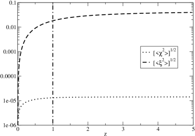
Figure 1.— Root-mean-squared fluctuation of $\chi$ (dotted) and $\xi$ (dashed) as a function of redshift.

Figure 1 shows the root-mean-squared fluctuation of $\chi$ (dotted) and $\xi$ (dashed) as a function of redshift. The vertical line approximately corresponds to the limit to which the Advanced Laser Interferometer Gravitational Observatory (LIGO) will be able to see for an optimally-oriented binary. We have here somewhat underestimated the $\left<\chi^{2}\right>^{1/2}$ term, as have neglected non-linear corrections to the power spectrum due to galaxy and cluster formation (Peacock and Dodds, 1996).

Data Analysis Implications. The detection of GWs by LISA or any other instrument will not be affected by matter inhomogeneities, since the phase correction accounts for a total phase shift that is extremized over during GW extraction. Parameter estimation, however, will clearly be affected by matter inhomogeneities. LISA is expected to be sensitive to the chirp mass and the luminosity distance to $\Delta\ln{\cal{M}}\sim 10^{-6}$ and $\Delta\ln D_{L}\sim 10^{-3}$ (Arun et al., 2007) for low-redshift sources ($z\sim 0.55$), but also sensitive to high redshift sources ($z\sim 5-10$) up to $\Delta\ln D_{L}\sim 10^{-2}$ (Hughes, 2002; Vecchio, 2004). Our calculations confirm that $\xi$ (associated with weak-lensing) will be a noise source in the use of standard sirens to measure the equation of state of dark energy through the redshifted luminosity distance (Kocsis et al., 2006).

Alternatively, one could view these effects as a new link between EM measurements of density inhomogeneities and LISA observations. In order to achieve this goal, however, one would first have to break the degeneracy between $({\cal{M}}_{z},z,\chi)$ or $(d_{L},z,\xi,\chi)$. Given a coincident EM and GW detection, one might be able to achieve just this, by electromagnetically determining the redshift and the component masses via host galaxy identification and correlations between galaxy luminosity and BH mass. Another possibility would be to use large scale structure observations to measure $\delta_{k}$ and predict $\chi$. Cosmologists already use large scale structure observations to predict the iSW term for the CMB (Afshordi, 2004). Such measurements would then open up, for the first time, studies of cross-correlations between GWs and large-scale structure surveys of dark matter (Crittenden and Turok, 1996) and possibly dark energy (Cooray et al., 2004). Furthermore, a detection of the cross-correlation between matter distribution and the GW iSW effect could potentially be another test of GR since it would show that GWs propagate in the same metric as EM radiation.

References

Hughes and Holz (2003)
S. A. Hughes and
D. E. Holz,
Class. Quant. Grav. 20,
S65 (2003).
Finn (1996)
L. S. Finn,
Phys. Rev. D53,
2878 (1996), gr-qc/9601048.
Flanagan and Hughes (1998)
E. E. Flanagan and
S. A. Hughes,
Phys. Rev. D 57,
4535 (1998).
Holz and Hughes (2005)
D. E. Holz and
S. A. Hughes,
ApJ 629, 15
(2005), arXiv:astro-ph/0504616.
Sachs and Wolfe (1967)
R. K. Sachs and
A. M. Wolfe,
Astrophys. J. 147,
73 (1967).
Rees and Sciama (1968)
M. J. Rees and
D. W. Sciama,
Nature 217,
511 (1968).
Giovannini (2005)
M. Giovannini,
Int. J. Mod. Phys. D14,
363 (2005), astro-ph/0412601.
Afshordi (2004)
N. Afshordi,
Phys. Rev. D70,
083536 (2004), astro-ph/0401166.
Isaacson (1968a)
R. A. Isaacson,
Phys. Rev. 166,
1263 (1968a).
Isaacson (1968b)
R. A. Isaacson,
Phys. Rev. 166,
1272 (1968b).
Pyne and Carroll (1996)
T. Pyne and
S. M. Carroll,
Phys. Rev. D 53, 2920
(1996), arXiv:astro-ph/9510041.