Cosmological constraints on rapid roll inflation

Abstract

We obtain cosmological constraints on models of inflation which exhibit rapid roll solutions. Rapid roll attractors exist for potentials with large mass terms and are thus of interest for inflationary model building within string theory. We constrain a general ansatz for the power spectrum arising from rapid roll inflation that, in the small field limit, can be associated with tree level hybrid potentials with variable mass terms and nonminimal gravitational coupling $\xi R\phi^{2}$. We consider perturbations generated through modulated reheating and/or curvaton mechanisms in place of the observationally unacceptable primary spectra generated by inflaton fluctuations in these models. The lack of a hierarchy amongst higher-order $k$-dependencies of the power spectrum results in models with potentially large runnings, allowing us to impose tight constraints on such models using CMB and LSS data. In particular, we find $n_{s}<1$ and $|\alpha|<0.01$. We conclude with a concrete realization of rapid roll inflation within warped throat brane inflation that is in good agreement with current data.

I Introduction

Recent years have seen steady progress in the development of inflation within string theory Cline:2006hu ; Kallosh:2007ig ; Burgess:2007pz ; McAllister:2007bg ; Baumann:2009ni . Inflation in string theory is beset by the $\eta$-problem Copeland:1994vg ; Kachru:2003sx , in which dimension 6, Planck-suppressed operators induce corrections to the inflaton mass of order the Hubble scale, $\delta m\sim\mathcal{O}(H)$. Such models are characterized by the parameter $\eta=M^{2}_{\rm Pl}\frac{V^{\prime\prime}}{V}\sim\mathcal{O}(1)$, preventing slow roll inflation. These corrections generically arise in the volume stabilization of brane inflation Kachru:2003sx , and a compelling solution to this problem remains an active area of research. This problem is compounded in models based on warped throat compactifications in which the length of the throat restricts the maximal field range Baumann:2006cd . It was earlier realized by Linde that it is possible to achieve significant efoldings of expansion even in the presence of large mass terms Linde:2001ae if the field enters a stage of rapid roll inflation. This choice of terminology will become clear below.

In this paper, we obtain observational constraints on models of inflation that undergo a period of rapid roll inflation. Typical examples of such potentials are those appearing in models of tree-level hybrid inflation, in which the field evolves along the rapid roll attractor, asymptotically approaching the minimum. These potentials give blue scalar spectra, which is observationally disfavored unless the tensor contribution is significant Komatsu:2008hk , and so we consider perturbations generated through other mechanisms, such as modulated reheating or the curvaton scenario. The light fields necessary for generating the primordial perturbations in these scenarios are abundant in string theory, making such mechanisms natural in this setting Kobayashi:2009cm .

We derive an analytical expression for the power spectrum, $P(k)$, arising from potentials of the form

$$V=V_{0}\left[1+\frac{1}{2}v_{2}\frac{\phi^{2}}{M_{\rm Pl}^{2}}+\mathcal{O}\left(\frac{\phi^{4}}{M_{\rm Pl}^{4}}\right)\right]$$ (1)

in which the field is restricted to the range $\phi\ll M_{\rm Pl}$. The formalism we develop is applicable to both minimally and nonminimally coupled scalar fields. The key result is that the power spectrum arising from modulated reheating and/or curvatons does not possess a hierarchy amongst low-order and high-order $k$-dependencies, in contrast to inflaton-generated perturbations. In fact, the higher-order runnings of the spectrum are completely determined by the spectral index, $n_{s}$, and first-order running, $\alpha=dn_{s}/d{\rm ln}k$, in the regime where Eq. (1) is justified. Using the latest CMB and LSS data, we perform a Bayesian analysis on this power spectrum. We compare these constraints with those obtained on a general ansatz for the power spectrum, $P(k)\propto k^{(n_{s}-1)+\frac{1}{2}\alpha{\rm ln}\frac{k}{k_{0}}}$, where the parameters $n_{s}$ and $\alpha$ are allowed to vary freely. The spectrum arising from rapid roll inflation is highly constrained relative to the generic parameterization, favoring $n_{s}<1$ and small running, $|\alpha|<0.01$.

Lastly, we present a concrete realization of rapid roll inflation within the context of warped throat brane inflation. We find that it is possible to obtain sufficient inflation in the presence of a range of mass terms, and the predictions of the model are in good agreement with the observational constraints we obtain in this paper.

In Section II, we review the concept of rapid roll inflation. In section III, we discuss the generation of perturbations in these models through either modulated reheating or curvatons, and derive an analytic expression for $P(k)$. In section IV we present the details of the Bayesian analysis, and report our constraints on the power spectrum. In Section V, we present a specific realization of rapid roll inflation within string theory.

II Rapid Roll Inflation

In this section we review the phenomenon of rapid roll inflation. To illustrate this concept, consider a minimally coupled scalar field $\phi$ with a potential of the form

$$V(\phi)=V_{0}+\frac{1}{2}m^{2}\phi^{2}.$$ (2)

This is a prototypical hybrid-type potential, in which inflation ends when an auxiliary field develops a tachyonic instability around $\phi\approx 0$. The equation of motion of a homogeneous scalar field in an FRW universe with this potential is

$$\ddot{\phi}+3H\dot{\phi}+m^{2}\phi=0.$$ (3)

When $H\approx$ const. we obtain the solution

$$\phi(t) = \phi_{+}e^{-r_{+}Ht}+\phi_{-}e^{-r_{-}Ht}$$ (4)

$$r_{\pm} = \frac{3}{2}\mp\sqrt{\frac{9}{4}-\frac{m^{2}}{H^{2}}},$$ (5)

where $\frac{m^{2}}{H^{2}}<\frac{9}{4}$. This is true for the potential Eq. (2) when $r_{+}^{2}\phi^{2}\ll M_{\rm Pl}^{2}$ and $m^{2}\phi^{2}\ll H^{2}M_{\rm Pl}^{2}$. The general solution is a superposition of both branches of Eq. (4) but at late times the field evolves along the $r_{+}$ branch, which is characterized by

$$\dot{\phi}\simeq-r_{+}H\phi.$$ (6)

Note that this behavior exists even if $m/H=O(1)$, i.e. one of the slow roll conditions is violated as $\eta=O(1)$. When $m/H=O(1)$, the dynamics defined by the solution Eq. (6) is termed rapid roll inflation. It tells us that the logarithmic variation of $\phi$ is set by the Hubble scale, or $\Delta\phi=O(\phi)$ in a Hubble time $\Delta t=H^{-1}$. This is in contrast to slow roll inflation, for which $|\dot{\phi}|\ll|H\phi|$. The number of efolds of expansion obtained during rapid roll is

$$N=\int Hdt\simeq-\frac{1}{r_{+}}\int\frac{d\phi}{\phi}=\frac{1}{r_{+}}{\rm ln}{\frac{\phi_{i}}{\phi_{f}}},$$ (7)

where $\phi_{i}$ and $\phi_{f}$ are the field values at the beginning and end of inflation. The spectral index of curvature perturbations from the inflaton is given by $n_{s}-1=2r_{+}$, and is therefore blue for this class of models GarciaBellido:1996ke . When $m/H=O(1)$, this means that we need other sources of curvature perturbations, such as curvaton and/or modulated reheating, to confront with observational data. (See the beginning of the next section for more about this point.)

Rapid roll solutions exist if a potential is approximated by (2) and if the field value is small enough. In order to make this statement quantitative, we consider more general potentials and introduce parameters to measure deviation from the form (2) and smallness of a field value. As shown in the appendix, the inflationary dynamics can be described by

$$cH\dot{\phi}(t)\simeq-V^{\prime}(\phi)$$ (8)

with $3M_{\rm Pl}^{2}H^{2}\simeq V$ if $\epsilon\ll 1$ and $|\bar{\eta}|\ll 1$ are satisfied. Here

$$\epsilon = \frac{M_{\rm Pl}^{2}}{2}\left(\frac{V^{\prime}}{V}\right)^{2},$$ (9)

$$\bar{\eta} = \eta+\frac{c^{2}}{3}-c,$$ (10)

$$\eta = M_{\rm Pl}^{2}\frac{V^{\prime\prime}}{V}$$ (11)

where $c$ is a constant of order unity. The value of $c$ is determined so that $|\bar{\eta}|$ is minimized in the duration of interest and that the corresponding solution is a dynamical attractor (see the appendix for details). For example, for the proto-type potential (2) with $\phi^{2}/M_{\rm Pl}^{2}$ small enough, there are two values of $c$ minimizing $|\bar{\eta}|$. The larger value corresponds to an attractor and agrees with the $r_{+}$ branch (6). Roughly speaking, $\bar{\eta}$ measures deviation of $V$ from the form (2) and $\epsilon$ measures smallness of the field.

Rapid roll inflation can also be manifested in models of inflation driven by non-minimally coupled scalar fields. In the rest of this section, for simplicity we consider a conformally coupled scalar field to drive rapid roll inflation. More systematic analysis with generic couplings will be presented in the next section. Thus, in the following we shall first write down some formulas with general couplings for later convenience and then restrict our consideration to the conformal coupling.

Consider the action of a non-minimally coupled scalar,

$$S=\int d^{4}x\sqrt{-g}\left[\frac{R}{2M_{\rm Pl}^{2}}-\frac{1}{2}\partial^{\mu}\phi\partial_{\mu}\phi-V(\phi)-\frac{1}{2}\xi R\phi^{2}\right].$$ (12)

In an FRW universe with $ds^{2}=-dt^{2}+a(t)^{2}d{\bf x}^{2}$, the resulting equations of motion are

$$3M_{\rm{Pl}}^{2}H^{2} = \frac{1}{2}\dot{\phi}^{2}+6\xi H\phi\dot{\phi}+3\xi\phi^{2}H^{2}+V(\phi),$$ (13)

$$M_{\rm Pl}^{2}\dot{H} = -\frac{1}{2}(1-2\xi)\dot{\phi}^{2}-4\xi H\phi\dot{\phi}-12\xi^{2}H^{2}\phi^{2}$$ (14)

$$- \xi\phi V^{\prime}(\phi)+\xi(1-6\xi)\phi^{2}\dot{H},$$

$$\ddot{\phi}+3H\dot{\phi} + 6\xi(\dot{H}+2H^{2})\phi+V^{\prime}(\phi)=0.$$ (15)

The value $\xi=\frac{1}{6}$ is known as conformal coupling. In this limit, the non-potential terms on the right hand side of Eq. (13) can be written as a perfect square,

$$3M^{2}_{\rm Pl}H^{2}=(\dot{\phi}+H\phi)^{2}+V(\phi).$$ (16)

Then, for constant potential, $V(\phi)=V_{0}$, the rapid roll solution $\dot{\phi}=-H\phi$ gives a de Sitter universe,

$$3M^{2}_{\rm Pl}H^{2}=V_{0}.$$ (17)

The existence of rapid roll solutions in this model could be understood by recalling that for $\dot{H}\approx 0$, the Ricci scalar $R\approx 12H^{2}$. Then for $\xi=\frac{1}{6}$, the coupling term in Eq. (12) forms an effective mass term $\simeq H^{2}\phi^{2}$, and we recover the potential Eq. (2). On the other hand, the exact de Sitter symmetry (17) in the conformally coupled frame could not have been guessed from the analysis for the minimally coupled models presented in the previous paragraphs. This difference between the conformal model with a flat potential and the minimal model with $m^{2}\simeq 2H^{2}$ becomes important when we discuss observables such as the spectral tilt of curvature perturbations generated from curvatons and/or modulated reheating since they reflect tiny deviations from the exact de Sitter symmetry. The conformally-coupled rapid-roll inflation was first investigated in Kofman:2007tr , where it was shown that rapid roll attractor solutions exist if a potential is flat enough. A small deviation of the non-minimal coupling strength $\xi$ from $1/6$ was considered in Kobayashi:2008rx . In the concrete example considered in Kofman:2007tr , the conformal coupling arises as the Hubble scale mass correction from volume stabilization in the KKLMMT Kachru:2003sx model and the potential is of the form

$$V(\phi)=V_{0}\left[1-\left(\frac{M_{\rm Pl}\Delta}{\phi}\right)^{4}\right],$$ (18)

where $\Delta$ is a dimensionless constant. This potential is flat except for very small values of $\phi$, and so the de Sitter solution holds across much of the inflationary trajectory.

In this paper, we seek constraints on rapid-roll inflation with not only minimal and conformal couplings but also arbitrary non-minimal coupling strengths.

III Primordial Perturbations

In this section we derive an analytic expression for the power spectrum generated by the rapid roll models introduced in the last section. An important aspect of this work is that we consider perturbations not generated by the inflaton itself, but rather from a mechanism such as modulated reheating Dvali:2003em ; Kofman:2003nx or curvatons Lyth:2001nq ; Moroi:2001ct ; Lyth:2002my . We do this for several reasons. The first is that spectra arising from the minimally coupled inflaton with potential Eq. (2) or flat potentials with almost conformal couplings $\xi\approx 1/6$ are blue ($n_{s}>1$) with small tensors. Observationally, blue spectra with low tensor-to-scalar ratio are disfavored Komatsu:2008hk . In addition to phenomenological motivations, such mechanisms are also attractive from a theoretical point of view. In particular, string theory provides natural candidates for the light moduli fields that generate perturbations in these alternative scenarios. Current work in which the curvaton is identified with an open string mode is under investigation kobayashi. The low energy scales required to suppress the inflaton perturbations on CMB scales are well tolerated by string inflation models, particularly brane inflation in warped throat compactifications. String inflation is also a pertinent place to realize the rapid roll inflation models considered in this paper.

III.1 Modulated Reheating and Curvatons

In order to reheat the universe, the inflaton field must undergo decays whose end products are the particles of the Standard Model. In supersymmetric and string theories, the couplings that facilitate these decays are not constants, but functions of scalar fields in the theory. If these fields are light during inflation ($m\ll H$), they will fluctuate in space with the result that the coupling constants (and hence decay rates) will become functions of space. Different parts of the universe thus decay and reheat at different times – the resulting spatial modulations in the reheat temperature give rise to energy density perturbations,

$$\frac{\delta T_{\rm RH}}{T_{\rm RH}}\propto\frac{\delta\rho}{\rho}.$$ (19)

For a light modulus field $\chi$, one finds Dvali:2003em

$$\frac{\delta\rho}{\rho}\propto\frac{\delta\chi}{M},$$ (20)

where $M$ is some mass scale. The key result is that the power spectrum of the resulting fluctuations is then $\propto H^{2}/M^{2}$, where $M$ can be taken sufficiently smaller than $M_{\rm Pl}$ to ensure that the inflaton perturbations are subdominant.

The primordial density perturbation may also be generated via the curvaton mechanism Lyth:2001nq ; Moroi:2001ct ; Lyth:2002my . The curvaton, $\sigma$, is a light scalar during inflation with an associated vacuum fluctuation, $\delta\sigma$. These fluctuations constitute a superhorizon isocurvature perturbation that grows during a post-inflationary radiation dominated phase. After curvaton decay, the perturbation is converted into an adiabatic mode with amplitude Lyth:2001nq

$$P_{\delta}\propto\frac{1}{\pi^{2}}\left(\frac{H}{\sigma}\right)^{2}.$$ (21)

If the curvaton is sufficiently light during inflation, $\sigma=const$ as a result of the Hubble drag and $P_{\delta}\sim H^{2}$. As in the case of modulated reheating by decaying light particles, the power spectrum is completely determined by the evolution of the Hubble parameter.

III.2 Power Spectrum

We now consider a rapid roll inflation driven by a non-minimally coupled inflaton $\phi$ and obtain an analytic expression for the power spectrum of curvature perturbations generated from curvaton/modulated reheating. Note that we consider minimally coupled field(s) responsible for curvatons/modulated reheating. This is possible if those fields responsible for curvature perturbations are associated with shift symmetries. For example, in the stringy setup presented in Kobayashi:2009cm , minimally coupled, light scalars can arise from angular isometries of the warped deformed conifold. Those light fields are responsible for curvaton/modulated reheating. On the other hand, we consider a non-minimally coupled scalar field as an inflaton. (Of course this class of models includes a minimally coupled inflaton as a special case.) As we shall see explicitly, observables such as the spectral tilt and its scale-dependence depend on the non-minimal coupling strength in a way that cannot be mimicked by a potential. Indeed, in the regime of validity of an approximation, we shall see that the scale-dependence of the power spectrum is characterized by two independent parameters, one of which is the non-minimal coupling strength and the other of which is a parameter of the potential. This explicitly shows that the effect of non-minimal coupling to observables cannot be mimicked by potentials in the regime of validity of the approximation.

Note again that we shall consider curvature perturbations generated from curvaton/modulated reheating. However, the background FRW evolutions is of course determined by the dynamics of the inflaton $\phi$, which is in general non-minimally coupled. Therefore, we consider a non-minimally coupled scalar field with a potential of the form

$$V = V_{0}\left[1+\sum_{n=1}^{\infty}\frac{v_{2n}}{(2n)!}x^{n}\right],$$ (22)

$$x \equiv \frac{\phi^{2}}{M_{\rm Pl}^{2}},$$ (23)

where $V_{0}$ and $v_{2n}$ are constants, and we suppose that $x\ll 1$. This is nothing but the Taylor expansion of a general potential with the $Z_{2}$ symmetry $\phi\to-\phi$, and can be considered as a simple generalization of (2). In the following, we shall perform a systematic analysis of the system by expansion w.r.t. $x$ ($\ll 1$). The scalar field satisfies the equations of motion Eqs. (13)-(15). Let us define $\Delta_{1}$ and $\Delta_{2}$ by

$$\Delta_{1} \equiv \frac{3M_{\rm Pl}^{2}H^{2}}{V_{0}}-\left[1+\sum_{n=1}^{N+1}\alpha_{2n}x^{n}\right],$$

$$\Delta_{2} \equiv \frac{\dot{\phi}}{H\phi}+\sum_{n=0}^{N}\beta_{2n}x^{n},$$ (24)

where $N$ is non-negative integer, and $\alpha_{2n}$ and $\beta_{2n}$ are constants to be determined. Note that the smallness of the parameters $\Delta_{1}$ and $\Delta_{2}$ guarantees the inflaton to be on the rapid roll attractor. (For the case of a minimally-coupled inflaton, each corresponds to approximations (69) and (70).) We shall determine $\alpha_{2n}$ with ($n=1,\cdots,N+1$) by demanding that

$$\Delta_{1}=O(x^{N+2}).$$ (25)

On the other hand, we demand that $\Delta_{2}$ satisfies

$$\frac{\dot{\Delta}_{2}}{H}+\gamma\Delta_{2}=O(x^{N+1})$$ (26)

for a positive constant $\gamma$. This condition uniquely determines $\beta_{2n}$ ($n=1,\cdots,N$) and $\gamma$ ($>0$). Note that the positivity of $\gamma$ is required by the stability of Eq. (26): $\Delta_{2}\to O(x^{N+1})$ as $a\to\infty$.

We now set $N=0$ to obtain the lowest order result. In principle, we can perform expansion up to larger $N$. For our purpose in the present paper, however, $N=0$ suffices. We follow the three steps to complete the program: First, we eliminate $\dot{H}$, $H^{2}$ and $\ddot{\phi}$ in Eqs. (25) and (26) by using Eqs. (14), (13) and (15), respectively. Next, we determine $\gamma$ by demanding that the coefficient of $\dot{\phi}$ in Eq. (26) after the first step should vanish. Lastly, we expand Eqs. (25) and (26) with respect to $x$ and solve them order by order.

The result is

$$\alpha_{2} = \left(\frac{1}{2}-2\xi\right)\beta_{0}-\xi,$$

$$\beta_{0} = \frac{3\pm\sqrt{9-12(v_{2}+4\xi)}}{2},$$

$$\gamma = 3-2\beta_{0}.$$ (27)

Since $\gamma$ is required to be positive, we need to choose the “$-$” sign for $\beta_{0}$. Thus,

$$\alpha_{2} = \left(\frac{1}{4}-\xi\right)\left[3-\sqrt{9-12(v_{2}+4\xi)}\right]-\xi,$$ (28)

$$\beta_{0} = \frac{3-\sqrt{9-12(v_{2}+4\xi)}}{2},$$ (29)

$$\gamma = \sqrt{9-12(v_{2}+4\xi)}.$$ (30)

The attractor equation Eq. (26) with $N=0$ and $\gamma>0$ implies that $\Delta_{2}\to O(\epsilon)$ as $a\to\infty$. Thus, we have $\dot{\phi}+\beta_{0}H\phi\simeq 0$. This gives

$$\phi\simeq\phi_{0}\left(\frac{a}{a_{0}}\right)^{-\beta_{0}},$$ (31)

where $\phi_{0}$ and $a_{0}$ are the values of $\phi$ and $a$ at $t=t_{0}$.

Then, Eq. (25) with $N=0$ implies that

$$P(k)\propto\left.\frac{3M_{\rm Pl}^{2}H^{2}}{V_{0}}\right|_{k=aH} \simeq 1+\alpha_{2}\frac{\phi_{0}^{2}}{M_{\rm Pl}^{2}}\left(\frac{k^{2}}{a_{0}^{2}H^{2}}\right)^{-\beta_{0}}$$

$$\simeq 1+\alpha_{2}\frac{\phi_{0}^{2}}{M_{\rm Pl}^{2}}\left(\frac{3M_{\rm Pl}^{2}k^{2}}{a_{0}^{2}V_{0}}\right)^{-\beta_{0}}$$

By choosing $a_{0}$ to be the scale factor at the pivot scale $k=k_{0}$, we obtain

$$P(k)\simeq\frac{P(k_{0})}{1+\alpha_{2}\frac{\phi_{0}^{2}}{M_{\rm Pl}^{2}}}\left[1+\alpha_{2}\frac{\phi_{0}^{2}}{M_{\rm Pl}^{2}}\left(\frac{k}{k_{0}}\right)^{-2\beta_{0}}\right],$$ (33)

where $\phi_{0}$ is the field value at the pivot scale. This can be written more concisely in the form

$$P(k)=\frac{P(k_{0})}{1+A}\left[1+A\left(\frac{k}{k_{0}}\right)^{-B}\right],$$ (34)

with

$$A = \alpha_{2}\frac{\phi_{0}^{2}}{M_{\rm Pl}^{2}}$$

$$= \left\{\left(\frac{1}{4}-\xi\right)\left[3-\sqrt{9-12(v_{2}+4\xi)}\right]-\xi\right\}\frac{\phi_{0}^{2}}{M_{\rm Pl}^{2}},$$

$$B = 2\beta_{0}=3-\sqrt{9-12(v_{2}+4\xi)}.$$ (36)

This is the main result of this section. Note that the scale-dependence of the power spectrum is characterized by the two parameters $A$ and $B$, which are expressed in terms of $\xi$ and $v_{2}$. It is easy to see that the effect of $\xi$ on ($A$, $B$) cannot be mimicked by $v_{2}$, and vice versa.

A unique aspect of power spectra arising from rapid roll inflation is the lack of a hierarchy amongst higher-order time derivatives of the Hubble parameter and higher-order $k$-dependencies of the power spectrum. Such hierarchies do exist in slow roll inflation, with the result that higher-order runnings are suppressed.

For example, in the case of nearly conformal inflation with $\xi=1/6+\delta\xi$ on a flat potential ($v_{2n}=0$), we have

$$A = -[\delta\xi+\mathcal{O}(\delta\xi^{2})]\frac{\phi_{0}^{2}}{M_{\rm Pl}^{2}},$$ (37)

$$B = 2(1+12\delta\xi)+\mathcal{O}(\delta\xi^{2}).$$ (38)

Then, the spectral index and runnings of the power spectrum Eq. (34) are

$$n_{s}-1 \simeq 2\delta\xi\frac{\phi_{0}^{2}}{M_{\rm Pl}^{2}},$$ (39)

$$\left.\left(\frac{d}{d{\rm ln}k}\right)^{2}{\rm ln}P(k)\right|_{k=k_{0}} \simeq -4\delta\xi\frac{\phi_{0}^{2}}{M_{\rm Pl}^{2}},$$

$$\vdots$$

$$\left.\left(\frac{d}{d{\rm ln}k}\right)^{m}{\rm ln}P(k)\right|_{k=k_{0}} \simeq -(-2)^{m}\delta\xi\frac{\phi_{0}^{2}}{M_{\rm Pl}^{2}}.$$ (41)

Note that all the derivatives are of the same order in $\delta\xi$ and $\frac{\phi_{0}^{2}}{M_{\rm Pl}^{2}}$, with higher-order runnings increasing in magnitude. It is therefore not possible to model these spectra as a Taylor expansion in ${\rm ln}k$, necessitating the use of Eq. (34) for imposing constraints.

In the case of perturbations generated through modulated reheating/curvatons, it is important to mention that minimally coupled models have power spectra proportional to the Hubble parameter formulated in the Einstein frame, $P(k)\propto H^{2}_{\rm E}$. In contrast, non-minimally coupled models have spectra related to the Jordan frame Hubble parameter, $P(k)\propto H^{2}_{\rm J}$. While this distinction is not very important when determining the duration of inflation ($H_{\rm E}$ and $H_{\rm J}$ differ by a factor $\phi^{2}/M_{\rm Pl}^{2}$), it is of importance for the observables, which are themselves of order $\phi^{2}/M_{\rm Pl}^{2}$.

IV Cosmological Constraints

We now obtain cosmological constraints on the power spectrum of curvature perturbations derived in the last section, Eq. (34). In order to ensure that the inflaton perturbations are suppressed on CMB scales, and for additional reasons that will become apparent in Section V, we consider low-scale inflation. We therefore do not include a gravitational wave contribution to the temperature anisotropy. We utilize Markov Chain Monte Carlo to obtain Bayesian parameter constraints from the 5^th-year WMAP cosmic microwave background data Hinshaw:2008kr ; Gold:2008kp ; Nolta:2008ih ; Dunkley:2008ie ; Komatsu:2008hk and the 4^th release SDSS Luminous Red Galaxy (LRG) galaxy power spectrum data AdelmanMcCarthy:2005se . We use the CosmoMC Lewis:2002ah code with a modified version of CAMB Lewis:1999bs in order to compute the $C_{\ell}$-spectra arising from Eq. (34). MCMC techniques Christensen:2000ji ; Christensen:2001gj ; Verde:2003ey ; Mackay generate samples from the likelihood of model parameters, $\mathcal{L}({\bf d}|{\bm{\theta}})$, where ${\bf d}$ represents the n-dimensional data and ${\bm{\theta}}$ the n-dimensional parameter vector. Via Bayes Theorem, the likelihood function relates any prior knowledge about the parameter values, $\pi({\bm{\theta}})$, to the posterior probability distribution,

$$p({\bm{\theta}}|{\bf d})=\frac{\mathcal{L}({\bf d}|{\bm{\theta}})\pi({\bm{\theta}})}{P({\bf d})}=\frac{\mathcal{L}({\bf d}|{\bm{\theta}})\pi({\bm{\theta}})}{\int\mathcal{L}({\bf d}|{\bm{\theta}})\pi({\bm{\theta}})d{\bm{\theta}}}.$$ (42)

The posterior probability distribution function of a single parameter $\theta_{i}$ is obtained by marginalizing $p({\bm{\theta}}|{\bf d})$ over the remaining parameters,

$$p(\theta_{i}|{\bf d})=\int p({\bm{\theta}}|{\bf d})d\theta_{1}\cdots d\theta_{i-1}d\theta_{i+1}\cdots d\theta_{n-1}.$$ (43)

We adopt a four parameter base cosmology: the baryon density $\Omega_{b}h^{2}$, the cold dark matter density $\Omega_{c}h^{2}$, the ratio of the sound horizon to the angular diameter distance at decoupling, $\theta_{s}$, and the optical depth to reionization, $\tau$. The power spectrum Eq. (34) is constrained by varying the parameters $P(k_{0})$, $A$, and $B$ directly in the Markov chains, at the pivot scale $k_{0}=0.002\,h{\rm Mpc}^{-1}$. We also marginalize over the contribution from the Sunyaev-Zeldovich effect by varying the amplitude $A_{\rm SZ}$ Komatsu:2002wc ; Komatsu:2008hk , assume purely adiabatic initial fluctuations, impose spatial flatness, and adopt a top-hat prior on the age of the universe: $t_{0}\in[10,20]$ Gyrs.

The posterior probability distribution in the directions of $A$ and $B$ is expected to be non-Gaussian. This is because the lines $A=0$ and $B=0$ give exactly scale invariant spectra, providing good fits to the data. The posterior thus has a high likelihood spine across the full prior of $A$ along $B=0$, and conversely across the full prior of $B$ along $A=0$. These spines are very narrow, since, for example, as one moves to larger values of $B$ along the $A=0$ line, a small step $\delta A$ gives a strongly non-power law spectrum. Therefore, while the posterior along these directions has high mean likelihood, the marginalized likelihood tends to be small. Sampling from this distribution thus poses a challenge, and we therefore utilize multicanonical sampling berg ; Gubernatis in lieu of the more standard Metropolis-Hastings algorithm. Multicanonical sampling is useful for probing into the tails of non-Gaussian distributions. We measure convergence across eight chains using the Gelman-Rubin R statistic ($R<1.1$).

The power spectrum Eq. (34) is not a freely tunable function. One requirement on the form of the spectrum is that the spacetime must be inflationary while astrophysical scales are generated. Otherwise, causally generated quantum fluctuations would not be stretched to super-horizon scales. Defining the parameter $\epsilon=-\dot{H}/H^{2}$, and with $P(k)\propto H^{2}$, we have

$$\epsilon=\frac{1}{2}\frac{d{\rm ln}P(k)}{d{\rm ln}k}\left[\frac{1}{2}\frac{d{\rm ln}P(k)}{d{\rm ln}k}-1\right]^{-1},$$ (44)

with

$$\frac{d{\rm ln}P(k)}{d{\rm ln}k}=-AB\left(\frac{k}{k_{0}}\right)^{-B}\left[1+A\left(\frac{k}{k_{0}}\right)^{-B}\right]^{-1}.$$ (45)

This is enforced by simply requiring that $\epsilon<1$ across the range of scales probed by cosmological observations, corresponding to wavenumbers $\Delta{\rm ln}k\approx 10$. Combinations of $A$ and $B$ which violate this condition are rejected from the sample by assigning such models very low likelihood.

As a means of comparison with the conventional parameterization, we transform the parameters $A$ and $B$ into the spectral parameters $n_{s}(k_{0})$ and $\alpha(k_{0})=dn_{s}(k_{0})/d{\rm ln}k$,

$$n_{s}(k_{0}) = 1-\frac{AB}{1+A},$$ (46)

$$\alpha(k_{0}) = \frac{AB^{2}}{(1+A)^{2}}.$$ (47)

While the prior $\pi(A,B)$ is chosen to be flat, the prior distribution $\pi(n_{s},\alpha)$ that results from this transformation is not. The Jacobian of the transformation

$$\pi(A,B)=\left|\frac{\partial(A,B)}{\partial(n_{s},\alpha)}\right|\pi(n_{s},\alpha),$$ (48)

is in fact zero at the point ($n_{s}=1$, $\alpha=0$), and so the prior is not well-defined at this point. While this presents a formal difficulty, it is of little consequence in practice since the Markov chains do not sample the neighborhood of this point with sufficient precision for the results to be affected by the prior in this area. We have verified that the posterior distribution is dominated by the likelihood across the prior range of $n_{s}$ and $\alpha$, and so $\pi(n_{s},\alpha)$ is effectively flat in this region.

Figure 1 displays the 1-$\sigma$ (68% CL) and 2-$\sigma$ (95% CL) error contours for the rapid roll model compared to the constraints obtained on $n_{s}$ and $\alpha$ when they are allowed to vary as free parameters (hereafter referred to as the plr model), as done in standard analyses by adopting the form

$${\rm ln}\frac{P(k)}{P(k_{0})}=(n_{s}-1){\rm ln}\frac{k}{k_{0}}+\frac{1}{2}\alpha{\rm ln}^{2}\frac{k}{k_{0}}.$$ (49)

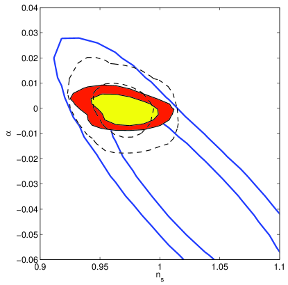
Figure 1: Marginalized constraints on rapid roll inflation as compared to constraints obtained on the spectral parameters in the standard definition (plr) Eq. (49). The blue contours denote 68% and 95% CL for the plr model with WMAP5+SDSS+ACBAR. The filled (orange-yellow) contours denote the same for the rapid roll model. The black dashed contours are constraints on rapid roll inflation with only WMAP5+SDSS. We shall see in figure 4 that, in D-brane inflation, these constraints for the rapid roll model are consistent with wide range of $|\dot{\phi}/H\phi|$.

The rapid roll model is significantly more predictive than the model-independent, plr spectrum with a preference for $n_{s}<1$ and small running. The marginalized constraints are given in Table 1.

Model	$n_{s}(k_{0})$	$\alpha(k_{0})$	$-2{\rm ln}\hat{\mathcal{L}}$
rapid roll	$0.972^{+0.022}_{-0.031}$	$-{5.01\times 10^{-3}}^{+0.01}_{-0.001}$	2693.5
plr	$1.04^{+0.16}_{-0.21}$	$-0.035^{+0.024}_{-0.025}$	2691.2

Table 1: Marginalized 2-$\sigma$ errors on the spectral parameters for the rapid roll model and the standard parameterization for WMAP5+SDSS+ACBAR.

The tight constraints on the rapid roll parameters are a result of the correlations between $n_{s}$, $\alpha$, and the infinite tower of higher-order $k$-dependent terms (e.g. Eq. (39)). The running of the running, $\beta=d\alpha/d{\rm ln}k$, and all terms of higher-order, are completely determined by $n_{s}$ and $\alpha$. For example,

$$\beta=\frac{\alpha^{2}}{n_{s}-1},$$ (50)

and so as the running is increased (for $n_{s}\neq 1$), $\beta$ likewise increases in magnitude. The tight constraints on $\alpha$ are therefore a direct result of the data’s intolerance to a large $\beta$. The constraints on the upper (lower) value of $n_{s}$ are a result of the data’s requirement that blue spectra be accompanied by significant negative (positive) running, as indicated by the black contours in Figure 1. The magnitude of running permitted in the rapid roll model is insufficient to accommodate very tilted spectra.

Of the spectra lying within the 2-$\sigma$ envelope, the most distinctive are those that exhibit a relatively abrupt increase in power on small scales at around $0.02\,h{\rm Mpc}^{-1}$. This $k$-dependence is a result of higher-order runnings. Since the WMAP data becomes noise-dominated at around the second peak, the addition of small-scale CMB measurements might have an effect on constraints. In Figure 2 we present the $C_{\ell}^{TT}$-spectrum of the best fit plr model (solid line) along with a model lying on the outskirts of the 2-$\sigma$ envelope (dashed line) when only WMAP5+SDSS are used. As suggested by Figure 2 and confirmed in Figure 1, the inclusion of the latest ACBAR data-set Reichardt:2008ay yields a distinctive improvement over the WMAP+SDSS only constraints, ruling-out such spectra at greater than 95% CL.

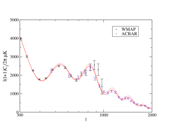
Figure 2: Best-fit plr model (red solid) as compared to a rapid roll spectrum lying at the edge of the 95% CL (red dashed). WMAP 5-year data (black points) and the 2008 ACBAR data (purple points) are included. The inclusion of ACBAR data imposes additional constraints on rapid roll models which exhibit higher-order running on small scales.

We also note that the rapid roll model does a poorer job of fitting the data than the plr model, with a difference in effective chi-square, $\Delta\chi^{2}=-2\Delta{\rm ln}\mathcal{L}\approx 2$, between them. Of course, this is not to say that the plr model is necessarily preferred by the data, since a proper comparison must also incorporate the number of degrees of freedom available to each model. However, this is not as simple as just counting the tunable parameters (both models have 8 – with 3 defining the power spectrum), since this number is not representative of model complexity, the quantity of interest when performing Bayesian model selection Kunz:2006mc . Rather, one should identify the number of parameters that are sufficiently constrained by the data, giving an effective number of parameters, $\mathcal{C}$ Kunz:2006mc ; Liddle:2007fy ,

$$\mathcal{C}=\overline{\chi^{2}(\bm{\theta})}-\chi^{2}(\hat{\bm{\theta}}),$$ (51)

where $\bm{\theta}$, is the parameter vector, the bar indicates an average, and the hat denotes the best-fit value. Using this prescription, we find that the plr model has 7 effective degrees of freedom, while the rapid roll model has 6.7. The fact that the rapid roll model has fewer effective parameters can be understood by examining the ansatz Eq. (34). As mentioned, both $A$ and $B$ give high mean likelihood across the full range of their respective priors. While the marginalized distribution of these parameters is well localized, there exist directions in the prior volume along which these parameters are unconstrained. The effective complexity criterion therefore does not count $A$ and $B$ as two free parameters, but rather a little less than this. It is therefore appropriate to conclude that current data does not single-out a preferred model, and it will be necessary for future experiments to improve our understanding of the power spectrum.

V Rapid Roll D-Brane Inflation

As a simple example of minimally coupled rapid-roll inflation (see also the appendix), let us consider D3/$\overline{\mathrm{D}3}$ brane inflation in a warped throat Kachru:2003sx . In this model, inflation is driven while a D3-brane is attracted towards an $\overline{\mathrm{D}3}$ sitting at the throat tip. The radial position $r$ of the D3 plays the role of the inflaton through $\phi\equiv\sqrt{T_{3}}r$, and the warped tension of the $\overline{\mathrm{D}3}$ sources inflation. It is known that the inflaton receives a large mass from moduli stabilization effects and that this tends to prevent slow-roll. Here, we also take into account corrections due to the throat coupling to the bulk Calabi-Yau space, which can be analysed using gauge/gravity duality Baumann:2008kq (see also Ceresole:1999zs ; Ceresole:1999ht ; Aharony:2005ez ). We consider the case where the leading bulk effect arises from a non-chiral operator of dimension $\Delta=2$ in the dual CFT, where the inflaton potential takes the form

$$V(\phi)=2h_{0}^{4}T_{3}\left\{1-\frac{3h_{0}^{4}T_{3}}{8\pi^{2}\phi^{4}}+\mu\left(\frac{\phi}{M_{\mathrm{Pl}}}\right)^{2}\right\},$$ (52)

where $h_{0}$ is the warping at the tip of the throat, $T_{3}$ is the brane tension, and the second term denotes the D3-$\overline{\mathrm{D}3}$ Coulombic interaction. When the bulk effects are absent, $\mu=1/3$ as was derived in the original KKLMMT paper Kachru:2003sx . The bulk effect introduces a negative contribution to the inflaton mass-squared, i.e. makes $\mu$ smaller than 1/3.

We restrict ourselves to the region $\phi^{2}\ll M_{\mathrm{Pl}}^{2}$. When the Coulombic attraction is negligible compared to the mass term:

$$\frac{M_{\mathrm{Pl}}^{2}h_{0}^{4}T_{3}}{\mu\phi^{6}}\ll 1,$$ (53)

we obtain rapid-roll inflation with

$$3M_{\mathrm{Pl}}^{2}H_{\mathrm{inf}}^{2}\simeq 2h_{0}^{4}T_{3}.$$ (54)

From Eqs. (9) and (11) one can estimate

$$\epsilon\simeq 2\mu^{2}\frac{\phi^{2}}{M_{\mathrm{Pl}}^{2}},\quad\eta\simeq 2\mu.$$ (55)

Then, setting

$$c=\frac{3+\sqrt{9-24\mu}}{2},$$ (56)

the inflationary attractor Eq. (8) gives

$$\frac{H}{\dot{\phi}}\simeq-\frac{3+\sqrt{9-24\mu}}{12\mu}\frac{1}{\phi}.$$ (57)

We note that the coefficient of $1/\phi$ agrees with $-1/\mu_{0}$ from Eq. (29) by setting $\xi=0$ and $v_{2}=2\mu$. Upon estimating the number of efoldings that can be obtained, one should note that the inflaton field range is bounded by the length of the throat Baumann:2006cd . Specifically, for throats supported by $N$ units of D3-brane charge, the bound gives $\phi_{\mathrm{UV}}\sim\sqrt{T_{3}}R$, where $R^{4}\sim g_{s}N\alpha^{\prime 2}$ Gubser:1998vd . Also, the end of inflation can be identified with the time when Eq. (53) breaks down, which gives

$$\phi_{\mathrm{end}}\sim\left(\frac{M_{\mathrm{Pl}}^{2}h_{0}^{4}T_{3}}{\mu}\right)^{1/6}.$$ (58)

Hence the maximum number of efoldings that can be obtained is

$$N_{\mathrm{max}}=\int^{\phi_{\mathrm{end}}}_{\phi_{\mathrm{UV}}}H\frac{d\phi}{\dot{\phi}}\\ \simeq\frac{3+\sqrt{9-24\mu}}{12\mu}\ln\left(\frac{\mu^{1/6}N^{1/4}g_{s}^{1/4}\alpha^{\prime 1/2}}{h_{0}^{2/3}L}\right).$$ (59)

Here we have used $T_{3}\sim 1/(g_{s}\alpha^{\prime 2})$ and $M_{\mathrm{Pl}}\sim L^{3}/(g_{s}\alpha^{\prime 2})$ where $L$ is the typical length scale of the six-dimensional bulk. The efolding number Eq. (59) depends sensitively on the mass parameter $\mu$, hence, one sees that even a slight effect from the bulk can change the duration of inflation drastically.

On the other hand, inflation should have started before the present Hubble scale exited the horizon. Therefore the required number of efoldings is at least

$$N\simeq\ln\left(10^{29}\frac{V_{\mathrm{inf}}^{1/4}}{M_{\mathrm{Pl}}}\right)\simeq\ln\left(10^{29}\frac{h_{0}g_{s}^{3/4}\alpha^{\prime 3/2}}{L^{3}}\right),$$ (60)

where we have assumed instantaneous (p)reheating, i.e. the universe was dominated by radiation right after inflation ended until matter-radiation equality. (This is realized in the case where there are D-branes left after inflation, since closed strings generated from D3-$\overline{\mathrm{D}3}$ annihilation soon decay into lighter states such as gravitons, KK modes, and open string modes on the residual D-branes, and then thermalize. See e.g. Chen:2006ni .)

In Figure 3, we present the ratio between the field range required to obtain sufficient inflation and the allowed range in the $\mu$ - $\log_{10}h_{0}$ plane. For example, if we take $g_{s}=0.1$, $N=10^{3}$, $L/\alpha^{\prime 1/2}=10$, and $h_{0}=10^{-11}$ (which set the inflation energy scale $V_{\mathrm{inf}}^{1/4}$ and the local string scale $h_{0}/\alpha^{\prime 1/2}$ to be of order 1 TeV, and $M_{\mathrm{Pl}}\alpha^{\prime 1/2}\sim 10^{4}$), then the necessary number of efoldings can be obtained when $\mu\lesssim 0.2$ is satisfied. As can be seen from Eqs. (59) and (60), smaller $h_{0}$ and $\mu$ are preferred for enough inflation to occur. Let us emphasize that the original Hubble scale mass (i.e. $\mu\sim 0.3$) need not be exactly cancelled for rapid roll inflation, provided there is sufficient warping of the throat.

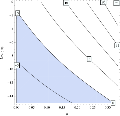
Figure 3: Contour plot of $\log_{10}(\phi_{H}/\phi_{UV})$, where $\phi_{H}$ is the inflaton field value when the present Hubble scale exited the horizon. $\phi_{H}$ is estimated by assuming that the inflaton potential Eq. (52) is valid throughout. The horizontal and vertical axes denote, respectively, $\mu$ and $\log_{10}h_{0}$. The other parameters are set to $g_{s}=0.1$, $N=1000$, and $L/\alpha^{\prime 1/2}=10$. Necessary number of efoldings can be obtained in the shaded region.

The inflaton field value when the pivot scale exited the horizon can similarly be estimated from Eqs. (59) and (60),

$$\frac{\phi_{0}}{M_{\mathrm{Pl}}}\sim\left(\frac{V_{\mathrm{inf}}}{\mu M_{\mathrm{Pl}}^{4}}\right)^{1/6}\left(10^{28}\frac{V_{\mathrm{inf}}^{1/4}}{M_{\mathrm{Pl}}}\right)^{\frac{12\mu}{3+\sqrt{9-24\mu}}}.$$ (61)

Note that for the pivot scale, the term inside the log in Eq. (60) differs by an order of magnitude.

The spectral index and its running of the Hubble-squared during inflation can be estimated from Eq. (34) with $\xi=0$ and $v_{2}=2\mu$, or from Eqs. (85) and (86),

$$n_{s}-1\simeq-\frac{18}{c^{2}}\cdot 2\mu^{2}\frac{\phi^{2}}{M_{\mathrm{Pl}}^{2}},$$ (62)

$$\frac{dn_{s}}{d\ln k}\simeq\frac{36}{c^{2}}(3-c)\cdot 2\mu^{2}\frac{\phi^{2}}{M_{\mathrm{Pl}}^{2}},$$ (63)

where the right hand sides are given at the moment of horizon crossing Eq. (61). One clearly sees a linear relation between Eqs. (62) and (63),

$$\frac{dn_{s}}{d\ln k}\simeq-\left(3-\sqrt{9-24\mu}\right)(n_{s}-1).$$ (64)

In Figure 4, we compare this prediction to the constraints obtained in Section IV. We plot the prediction Eq. (64) for the values $\mu=0.001$, $\mu=0.05$, and $\mu=0.3$ to illustrate the range of values of $\alpha$ and $n_{s}$ consistent with current data. These values correspond to $|\dot{\phi}/H\phi|\simeq 0.002$, $|\dot{\phi}/H\phi|\simeq 0.1$, $|\dot{\phi}/H\phi|\simeq 0.8$, respectively. (See (57).) For fixed $\mu$, each prediction is a function of $\phi_{0}$ which depends on the inflationary energy scale. The rapid roll brane inflation model is consistent with current data for a wide range of $\mu$ and, thus, $\dot{\phi}/H\phi$ and $\eta$.

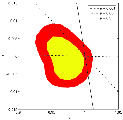
Figure 4: Prediction of the rapid roll brane model Eq. (64) for the values $\mu=0.001$, $\mu=0.05$, and $\mu=0.3$ compared to the constraints obtained in Section IV. These values correspond to $|\dot{\phi}/H\phi|\simeq 0.002$, $|\dot{\phi}/H\phi|\simeq 0.1$, $|\dot{\phi}/H\phi|\simeq 0.8$, respectively.

Finally, we mention that even though we have treated D-brane inflation as a minimally coupled model with Hubble scale mass, interpreting the mass as arising from the inflaton’s conformal coupling to gravity does not make much difference for the inflaton dynamics and the efolding number that can be obtained. However, it does make distinct differences for the spectral index and its running of the Hubble-squared, for reasons discussed at the end of Section III. One can explicitly see this for the D-brane inflation case by comparing the above results with that of Kobayashi:2008rx .

VI Conclusions

We have obtained cosmological constraints on rapid roll models of inflation. Rapid roll solutions exist as attractors for tree-level hybrid-type potentials with a range of mass terms, with both minimal and nonminimal gravitational couplings. Such solutions are therefore relevant to model building in string theory. We considered perturbations generated through modulated reheating and/or the curvaton scenario instead of the observationally unacceptable inflaton-generated perturbations in these models. We obtained an analytic expression for the power spectrum in this case,

$$P(k)=\frac{P(k_{0})}{1+A}\left[1+A\left(\frac{k}{k_{0}}\right)^{-B}\right],$$ (65)

observing a lack of a hierarchy amongst lower-order and higher-order $k$-dependencies. We have performed a Bayesian analysis on this power spectrum using the latest CMB and LSS data. The higher-order runnings are fully determined by $n_{s}$ and $\alpha$, and so these parameters are tightly constrained relative to general power-law + running spectra. We find that rapid roll models are constrained to have $n_{s}<1$ and small running, $|\alpha|<0.01$. These tight predictions make possible the falsifiability of rapid roll inflation with upcoming CMB missions. The higher-order runnings that occur in these spectra might also be further constrained via upcoming astrophysical probes, such as the 21-cm line of neutral hydrogen clouds.

We also construct a realistic model of rapid roll brane inflation. We find that it is possible to obtain sufficient inflation even in the presence of the large mass terms that arise from moduli stabilization in these models. The power spectrum generated by this model is in good agreement with the constraints obtained in this work, across a range of mass scales. Therefore, while the inflaton-generated perturbations of such models are not observationally viable, the spectra generated through other means, such as modulated reheating or curvatons, breathe new life into these constructions. Additionally, the tight constraints imposed on these spectra suggest that future CMB data has the potential to further restrict them, or rule such models out entirely.

VII acknowledgements

The calculations were performed by the EUP cluster system installed at Graduate School of Frontier Sciences, University of Tokyo. We thank Damien Easson for comments on a draft version of this paper. The work of S.M. was supported in part by MEXT through a Grant-in-Aid for Young Scientists (B) No. 17740134, and by JSPS through a Grant-in-Aid for Creative Scientific Research No. 19GS0219. This work was supported by World Premier International Research Center Initiative (WPI Initiative), MEXT, Japan.

Appendix A Discussions on Minimally Coupled Rapid-Roll Inflation

We investigate the dynamics of a rapid-rolling inflaton which minimally couples to gravity. The calculations carried out in this appendix is analogous to that of Kobayashi:2008rx where a conformally coupled inflaton was studied.

A.1 Conditions for Rapid-Roll Inflation

We consider a minimally coupled inflaton with the Lagrangian

$$\mathcal{L}=\sqrt{-g}\left[\frac{M_{\mathrm{Pl}}^{2}}{2}R-\frac{1}{2}g^{\mu\nu}\partial_{\mu}\phi\partial_{\nu}\phi-V(\phi)\right].$$ (66)

Choosing a flat FRW background, we obtain the Friedmann equation

$$3M_{\mathrm{Pl}}^{2}H^{2}=\frac{1}{2}\dot{\phi}^{2}+V(\phi),$$ (67)

and the equation of motion of $\phi$,

$$\ddot{\phi}+3H\dot{\phi}+V^{\prime}(\phi)=0.$$ (68)

We claim that during inflation, the inflaton dynamics is well described by the following approximations

$$3M_{\mathrm{Pl}}^{2}H^{2}\simeq V,$$ (69)

$$cH\dot{\phi}\simeq-V^{\prime},$$ (70)

where $c$ is a dimensionless constant.

Let us define the following parameters,

$$\epsilon\equiv\frac{M_{\mathrm{Pl}}^{2}}{2}\left(\frac{V^{\prime}}{V}\right)^{2},\quad\bar{\eta}\equiv\eta+\frac{c^{2}}{3}-c,$$ (71)

where

$$\eta\equiv M_{\mathrm{Pl}}^{2}\frac{V^{\prime\prime}}{V}.$$ (72)

Then the necessary conditions for the approximate relations (69) and (70) to hold can be derived, respectively, as

$$\frac{3}{c^{2}}\epsilon\ll 1,\quad\frac{3}{c^{2}}\left|3\epsilon-\bar{\eta}\right|\ll 1.$$ (73)

Note that we have taken a time-derivative of both sides of the approximate relation (70) and then substituted it into (68) in order to derive the necessary condition for (70). When $c\sim\mathcal{O}(1)$, the necessary conditions (73) reduce to simple forms

$$\epsilon\ll 1,\quad\left|\bar{\eta}\right|\ll 1.$$ (74)

This shows that the parameters which should be minimized in order to realize inflation are $\epsilon$ and $\bar{\eta}$ (instead of $\epsilon$ and $\eta$). The constant $c$ in (70) is the largest constant that minimizes $\bar{\eta}$, as we will show in the next section.

A.2 Stability of the Attractor

Let us define $\beta$ to parametrize the validness of the attractor (70) as

$$cH\dot{\phi}=-V^{\prime}(1+\beta).$$ (75)

We derive an evolution equation of $\beta$ in this section.

Some useful relations are

$$\Sigma\equiv\frac{3M_{\mathrm{Pl}}^{2}H^{2}}{V}\\ =\frac{1}{2}\left\{1+\sqrt{1+\frac{12(1+\beta)^{2}}{c^{2}}\epsilon}\right\}=1+\mathcal{O(\epsilon)},$$ (76)

$$\frac{\dot{\phi}^{2}}{V}=2\left(\Sigma-1\right),\quad\frac{\dot{H}}{H^{2}}=-\frac{3(\Sigma-1)}{\Sigma}.$$ (77)

Then by time-differentiating both sides of (75), one obtains

$$\frac{\dot{\beta}}{H}=\frac{3}{\Sigma}\left\{1-2\Sigma+\frac{1+\beta}{c}\eta\right\}(1+\beta)+c\\ =\beta(3-2c)+\beta^{2}(3-c)+\mathcal{O}(\epsilon,\,\bar{\eta}).$$ (78)

Once $\beta$ becomes small, the far right hand side is dominated by the linear term (i.e. $\beta(3-2c)$). One can see that as long as

$$3-2c<0,$$ (79)

$\beta$ damps as the universe expands, and eventually its value settles down to that corresponding to the source terms,

$$\beta=\mathcal{O}(\epsilon,\,\bar{\eta}).$$ (80)

Hence the the condition (79) is required for the relations (69) and (70) to be an inflationary attractor.

Next we study the values of $c$ chosen for inflation. As we stressed in the previous section, $c$ is a constant which minimizes $\bar{\eta}/c^{2}$.

Case Study: negligible $\eta$

This corresponds to the familiar slow-roll inflation. Here $\bar{\eta}/c^{2}=0$ gives $c=3$, which realizes the slow-roll approximations. It is clear that the stability condition (79) is satisfied.

Case Study: non-negligible constant $\eta$

$\bar{\eta}/c^{2}=0$ is solved by

$$c=\frac{3\pm\sqrt{9-12\eta}}{2}\equiv c_{\pm}.$$ (81)

Since $3-2c_{\pm}=\mp\sqrt{9-12\eta}\lessgtr 0$, one sees from (79) that the larger solution $c_{+}$ is chosen for the inflationary attractor,

$$c=\frac{3+\sqrt{9-12\eta}}{2}.$$ (82)

It should also be noted that $\eta\leq 3/4$ needs to be satisfied.

A.3 Scale Dependence of $H^{2}$

By using the relations in the previous section and considering $\beta$ to be damped to (80), one can compute the time differentiations of the Hubble parameter,

$$\frac{\dot{H}}{H^{2}}=-\frac{9}{c^{2}}\epsilon+\mathcal{O}(\bar{\eta}\epsilon,\,\epsilon^{2}),$$ (83)

$$\frac{1}{H}\left(\frac{\dot{H}}{H^{2}}\right)^{\cdot}=-\frac{18}{c^{2}}(c-3)\epsilon+\mathcal{O}(\bar{\eta}\epsilon,\,\epsilon^{2}).$$ (84)

Especially, the spectral index and its running of the Hubble-squared are ($k=aH$),

$$n_{s}-1=\frac{d\ln H^{2}}{d\ln k}=2\frac{\dot{H}}{H^{2}}\left(1+\frac{\dot{H}}{H^{2}}\right)^{-1}\\ =-\frac{18}{c^{2}}\epsilon+\mathcal{O}(\bar{\eta}\epsilon,\,\epsilon^{2}),$$ (85)

$$\frac{dn_{s}}{d\ln k}=2\left(1+\frac{\dot{H}}{H^{2}}\right)^{-3}\frac{1}{H}\left(\frac{\dot{H}}{H^{2}}\right)^{\cdot}\\ =\frac{36}{c^{2}}(3-c)\epsilon+\mathcal{O}(\bar{\eta}\epsilon,\,\epsilon^{2}).$$ (86)

For inflaton potentials of the form (1), these expressions match with what follows from Eq. (34) with $\xi=0$.

References

- (1) J. M. Cline, arXiv:hep-th/0612129.
- (2) R. Kallosh, Lect. Notes Phys. 738, 119 (2008) [arXiv:hep-th/0702059].
- (3) C. P. Burgess, PoS P2GC, 008 (2006) [Class. Quant. Grav. 24, S795 (2007)] [arXiv:0708.2865 [hep-th]].
- (4) L. McAllister and E. Silverstein, Gen. Rel. Grav. 40, 565 (2008) [arXiv:0710.2951 [hep-th]].
- (5) D. Baumann and L. McAllister, arXiv:0901.0265 [hep-th].
- (6) E. J. Copeland, A. R. Liddle, D. H. Lyth, E. D. Stewart and D. Wands, Phys. Rev. D 49, 6410 (1994) [arXiv:astro-ph/9401011].
- (7) S. Kachru, R. Kallosh, A. Linde, J. M. Maldacena, L. P. McAllister and S. P. Trivedi, JCAP 0310, 013 (2003) [arXiv:hep-th/0308055].
- (8) D. Baumann and L. McAllister, Phys. Rev. D 75, 123508 (2007) [arXiv:hep-th/0610285].
- (9) A. Linde, JHEP 0111, 052 (2001) [arXiv:hep-th/0110195].
- (10) L. Boubekeur and D. H. Lyth, JCAP 0507, 010 (2005) [arXiv:hep-ph/0502047].
- (11) E. Komatsu et al. [WMAP Collaboration], arXiv:0803.0547 [astro-ph].
- (12) J. Garcia-Bellido and D. Wands, Phys. Rev. D 54, 7181 (1996) [arXiv:astro-ph/9606047].
- (13) W. H. Kinney, Phys. Rev. D 72, 023515 (2005) [arXiv:gr-qc/0503017].
- (14) K. Tzirakis and W. H. Kinney, Phys. Rev. D 75, 123510 (2007) [arXiv:astro-ph/0701432].
- (15) L. Kofman and S. Mukohyama, Phys. Rev. D 77, 043519 (2008) [arXiv:0709.1952 [hep-th]].
- (16) T. Kobayashi and S. Mukohyama, Phys. Rev. D 79, 083501 (2009) [arXiv:0810.0810 [hep-th]].
- (17) G. Dvali, A. Gruzinov and M. Zaldarriaga, Phys. Rev. D 69, 023505 (2004) [arXiv:astro-ph/0303591].
- (18) L. Kofman, arXiv:astro-ph/0303614.
- (19) D. H. Lyth and D. Wands, Phys. Lett. B 524, 5 (2002) [arXiv:hep-ph/0110002].
- (20) T. Moroi and T. Takahashi, Phys. Lett. B 522, 215 (2001) [Erratum-ibid. B 539, 303 (2002)] [arXiv:hep-ph/0110096].
- (21) D. H. Lyth, C. Ungarelli and D. Wands, Phys. Rev. D 67, 023503 (2003) [arXiv:astro-ph/0208055].
- (22) T. Kobayashi and S. Mukohyama, arXiv:0905.2835 [hep-th].
- (23) G. Hinshaw et al. [WMAP Collaboration], arXiv:0803.0732 [astro-ph].
- (24) B. Gold et al. [WMAP Collaboration], arXiv:0803.0715 [astro-ph].
- (25) M. R. Nolta et al. [WMAP Collaboration], arXiv:0803.0593 [astro-ph].
- (26) J. Dunkley et al. [WMAP Collaboration], arXiv:0803.0586 [astro-ph].
- (27) J. K. Adelman-McCarthy et al. [SDSS Collaboration], Astrophys. J. Suppl. 162, 38 (2006) [arXiv:astro-ph/0507711].
- (28) A. Lewis and S. Bridle, Phys. Rev. D 66, 103511 (2002) [arXiv:astro-ph/0205436].
- (29) A. Lewis, A. Challinor and A. Lasenby, Astrophys. J. 538, 473 (2000) [arXiv:astro-ph/9911177].
- (30) N. Christensen and R. Meyer, arXiv:astro-ph/0006401.
- (31) N. Christensen, R. Meyer, L. Knox and B. Luey, Class. Quant. Grav. 18, 2677 (2001) [arXiv:astro-ph/0103134].
- (32) L. Verde et al. [WMAP Collaboration], Astrophys. J. Suppl. 148, 195 (2003) [arXiv:astro-ph/0302218].
- (33) D. MacKay, Information Theory, Inference, and Learning Algorithms, Cambridge University Press, Cambride, U.K. (2003)
- (34) E. Komatsu and U. Seljak, Mon. Not. Roy. Astron. Soc. 336, 1256 (2002) [arXiv:astro-ph/0205468].
- (35) B. A. Berg, Fields Inst. Commun. 26, 1 (2000)
- (36) J. Gubernatis and N. Hatano, Computing in Science & Engineering 2, 95 (2002)
- (37) C. L. Reichardt et al., Astrophys. J. 694, 1200 (2009) [arXiv:0801.1491 [astro-ph]].
- (38) M. Kunz, R. Trotta and D. Parkinson, Phys. Rev. D 74, 023503 (2006) [arXiv:astro-ph/0602378].
- (39) A. R. Liddle, Mon. Not. Roy. Astron. Soc. Lett. 377, L74 (2007) [arXiv:astro-ph/0701113].
- (40) D. Baumann, A. Dymarsky, I. R. Klebanov, J. M. Maldacena, L. P. McAllister and A. Murugan, JHEP 0611, 031 (2006) [arXiv:hep-th/0607050].
- (41) D. Baumann, A. Dymarsky, I. R. Klebanov, L. McAllister and P. J. Steinhardt, Phys. Rev. Lett. 99, 141601 (2007) [arXiv:0705.3837 [hep-th]].
- (42) A. Krause and E. Pajer, JCAP 0807, 023 (2008) [arXiv:0705.4682 [hep-th]].
- (43) D. Baumann, A. Dymarsky, I. R. Klebanov and L. McAllister, JCAP 0801, 024 (2008) [arXiv:0706.0360 [hep-th]].
- (44) D. Baumann, A. Dymarsky, S. Kachru, I. R. Klebanov and L. McAllister, JHEP 0903, 093 (2009) [arXiv:0808.2811 [hep-th]].
- (45) A. Ceresole, G. Dall’Agata, R. D’Auria and S. Ferrara, Phys. Rev. D 61, 066001 (2000) [arXiv:hep-th/9905226].
- (46) A. Ceresole, G. Dall’Agata and R. D’Auria, JHEP 9911, 009 (1999) [arXiv:hep-th/9907216].
- (47) O. Aharony, Y. E. Antebi and M. Berkooz, Phys. Rev. D 72, 106009 (2005) [arXiv:hep-th/0508080].
- (48) X. Chen and S. H. Tye, JCAP 0606, 011 (2006) [arXiv:hep-th/0602136].
- (49) S. S. Gubser, Phys. Rev. D 59, 025006 (1999) [arXiv:hep-th/9807164].