Experiment Study of Entropy Convergence of Ant Colony Optimization

Abstract

Ant colony optimization (ACO) has been applied to the field of combinatorial optimization widely. But the study of convergence theory of ACO is rare under general condition. In this paper, the authors try to find the evidence to prove that entropy is related to the convergence of ACO, especially to the estimation of the minimum iteration number of convergence. Entropy is a new view point possibly to studying the ACO convergence under general condition.

I Introduction

ACO is a recently developed, population-based approach presented by M. Dorigo and A. Colorni etc. al., it was inspired by the ants’ foraging behavior in 1991 Dorigo ; Colorni ; Dorigo1 . Ant System (AS) was first introduced in three different versions Dorigo ; Colorni ; Dorigo1 , they were called ant-density, ant-quantity, and ant-cycle. Ant Colony System (ACS) has been introduced in Dorigo2 ; Cambardella to improve the performance of AS. Later, AS and ACS developed into a unifying framework to solve combinatorial optimization problems Dorigo3 ; Dorigo4 ,  and the framework is often called Ant Colony Optimization (ACO). ACO has been applied to solve optimization problemsBall1 ; Ball2 , such as Traveling Salesman Problem (TSP)Dorigo2 ; Cambardella1 , Quadratic Assignment Problem(QAP)Cambardella2 , Job-shop Scheduling Problem(JSP)Cambardella1 , Vehicle Routing Problem( VRP)Bullnheimer ; Forsyth and Data Mining(DM)Rafael . The high performance of ACO and its wide application make it as famous as other optimization algorithms, such as Simulated Annealing (SA)Kirkpatrick , Tabu Search (TS)Glover , Genetic Algorithms (GA)Golderg , and so on.

The study of ACO theory is necessary but rare. W. J. Gutjahr studies the convergence of ACO under some conditions by Graph TheoryGutjahr , which is called Graph-Based Ant System (GBAS). GBAS maps a feasible solution of optimization problem to a route in a directed graph. T. St$\overset{..}{u}$ezle and M. Dorigo proved the existence of the ACO convergence under two conditions, one is to only update the pheromone of the shortest route generated at each iteration step, the other is that the pheromone on all routes has lower bound Stuezle . J. H. Yoo analyzes the convergence of a kind of distributed ants routing algorithm by the method of artificial intelligence Yoo ; Yoo1 . Sun analyzes the convergence of a simple ant algorithm by Markov ProcessSun . Ding presents a hybrid algorithm of ACO and genetic algorithm, and analyzes the convergence by Markov theory Ding . Hou presents a special ACO algorithm and proves its convergence by fixed-point theorem Hou .

The ways of studying ACO convergence are rare, such as Markov theory, Graph Theory, and so on. And only the results with some constraint conditions are obtained currently, and the result with no constraint condition is still unknown. The motivation of this paper is to explore the way to study ACO convergence under no constraint condition.

II Framework of ACO

In the 1990s, ACO was introduced as a novel nature-inspired method for the solution of hard combinatorial optimization problems (Dorigo, 1992; Dorigo et al., 1996, 1999; Dorigo and St$\overset{..}{u}$ezle, 2004). The inspiring source of ACO is the foraging behavior of real ants. When searching for food, ants initially explore the area surrounding their nest in a random manner. As soon as an ant finds a food source, it remembers the route passed by and carries some food back to the nest. During the return trip, the ant deposits pheromone on the ground. The deposited pheromone, guides other ants to the food source. And it has been shown (Goss et al., 1989), indirect communication among ants via pheromone trails enables them to find the shortest routes between their nest and food sources.

The framework of ACO is shown in Algorithm 1, and it is applied to solve Travel Salesman Problem (TSP). Where TSP can be explained as follows: for a given set of cities, the task of TSP is to find the cheapest route of visiting all of the cities and returning to starting point, provided each city is only visited once.

Algorithm 1

Step1. Initialization: Initialize pheromone of all edges among cities. And put $m$ ants at different cities randomly. Pre-assign an iteration number $N_{C_{\max}}$ and let $t=0$, where $t$ denotes the $t-th$ iteration step.

Step2. while($t<N_{C_{\max}}$)

{

Step2.1. All ants select its next city according to the transition probability defined in formula (1), which is the probability that the $k-th$ ant selecting the edge from $i-th$ city to $j-th$ city.

$$p_{ij}^{(k)}(t)=\left\{\begin{tabular}[]{ccc}$\frac{\tau_{ij}^{\alpha}(t).\eta_{ij}^{\beta}}{\underset{s\in allowed_{k}}{\sum}\tau_{is}^{\alpha}(t).\eta_{is}^{\beta}}$&$if$&$j\in allowed_{k}$\\ $0$&\lx@intercol\hfil$otherwise$\hfil\lx@intercol\end{tabular}\right.$$ (1)

, where $allowed_{k}$ denotes the set of cities that can be accessed by the $k-th$ ant; $\tau_{ij}(t)$ is the pheromone value of the edge ($i,j$); $\eta_{ij}$ is a local heuristic function defined as

$$\eta_{ij}=\frac{1}{d_{ij}}$$ (2)

, where $d_{ij}$ is the distance between the $i-th$ city and the $j-th$ city; the parameters $\alpha$ and $\beta$ determine the relative influence of the trail strength and the heuristic information respectively.

Step2.2. After all ants finish their travels, all pheromone values $\tau_{ij}(t)$ are updated according to formula (3).

$$\tau_{ij}(t+1)=(1-\rho)\cdot\tau_{ij}(t)+\Delta\tau_{ij}(t)$$ (3)

$$\Delta\tau_{ij}(t)=\overset{m}{\underset{k=1}{\sum}}\Delta\tau_{ij}^{(k)}(t)$$ (4)

$$\Delta\tau_{ij}^{(k)}(t)=\left\{\begin{tabular}[]{ccc}$\frac{Q}{L^{(k)}(t)}$&$if$&$the$ $k-th$ $ant$ $pass$ $edge$ $(i,j)$\\ $0$&\lx@intercol\hfil$otherwise$\hfil\lx@intercol\end{tabular}\right.$$ (5)

,where $L^{(k)}(t)$ is the length of the route passed by the $k-th$ ant; $\rho$ is the persistence ratio of the trail (thus, ($1-\rho$) corresponds to the evaporation ratio); $Q$ denotes constant quantity of pheromone.

Step2.3. Increase iteration number, i.e., $t\leftarrow t+1$.

}

Step3. End procedure and select the route which has shortest length as the output.

III The Statistical Feature of The Solutions of ACO

III.1 Definition of Symbols

ACO solving the problem of TSP is the model in this paper. Suppose the $m$ ants are $a_{1}$, $a_{2}$, ……, $a_{m}$. At the $t-th$ iteration step, ant $a_{i}$ selects route $r_{i}^{(t)}$ and it has length $L_{i}^{(t)}$. After all ants finish their $t-th$ travels,  there are totally amount of pheromone $f_{i}^{(t)}=\underset{(k,j)\in r_{i}^{(t)}}{\sum\tau_{kj}(t)}$ depositing on router $r_{i}^{(t)}$, where $\tau_{kj}(t)$ denotes pheromone depositing at the edge $(k,j)$ by all ants.

Definition 1 (Pheromone Probability):

$$p_{i}^{(t)}=\frac{f_{i}^{(t)}}{\overset{m}{\underset{j=1}{\sum}}f_{j}^{(t)}}$$ (6)

In formula (6), $\overset{m}{\underset{j=1}{\sum}}f_{j}^{(t)}$ represents the sum of pheromone of all routes. $p_{i}^{(t)}$ represents the ratio of pheromone that is assigned at the $i-th$ route $r_{i}^{(t)}$. The more big the ratio $p_{i}^{(t)}$ is, the more possibly the edges of route $r_{i}^{(t)}$ are selected by ants at the next iteration step. That is, $p_{i}^{(t)}$ is a probability which will affect the route selection of ant at the next iteration step. $p_{i}^{(t)}$ is called as pheromone probability, and Fig.1 diagrammatizes it.

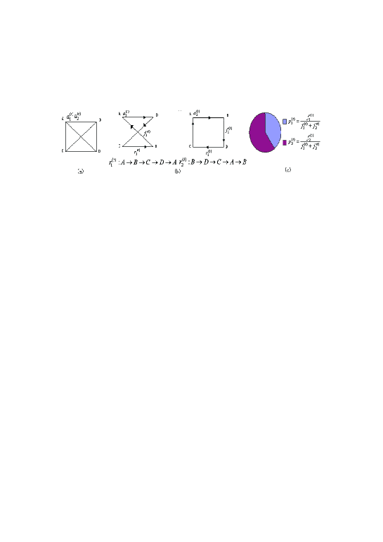
Figure 1: The Schematic of pheromone probability $p_{i}^{(t)}$. (a) There is a complete graph with four vertices, two ants $a_{1}^{(t)}$ and $a_{2}^{(t)}$ act on it at the $t-th$ iteration step. (b) Two ants $a_{1}^{(t)}$ and $a_{2}^{(t)}$ select two routes $r_{1}^{(t)}$ and $r_{2}^{(t)}$ respectively. Every edge of route $r_{1}^{(t)}$ contains pheromone , $f_{1}^{(t)}$ represents the sum of pheromone on all edges of route $r_{1}^{(t)}$. As same, $f_{2}^{(t)}$ represents the sum of pheromone on all edges of route $r_{2}^{(t)}$. (c) There are two routes $r_{1}^{(t)}$ and $r_{2}^{(t)}$ totally, $p_{i}^{(t)}$ represents the ratio of pheromone assigned at route $r_{i}^{(t)}$. The more bigger ratio $p_{i}^{(t)}$ is, the more possibly the edges at route $r_{i}^{(t)}$ were selected by ants at the next iteration step. That is, $p_{i}^{(t)}$ is a probability which will affect the route selection of ants at the next iteration.

Definition 2 (Route Length Set): At the $t-th$ iteration step, $m$ ants select $m$ routes. The set of route lengths is denoted as

$$L\_Set^{(t)}=\{L_{1}^{(t)},L_{2}^{(t)},...,L_{i}^{(t)},...,L_{m}^{(t)}\}$$

Definition 3 (Pheromone Probability Set): The set of pheromone probabilities is defined as

$$P\_Set^{(t)}=\{p_{1}^{(t)},p_{2}^{(t)},...,p_{i}^{(t)},...,p_{m}^{(t)}\}$$

III.2 Statistical Features of Route Length Set

At the $t-th$ iteration step, the $i-th$ ant $a_{i}$ selects route $r_{i}^{(t)}$, where $i=1,2,...,m$. And route $r_{i}^{(t)}$ has length $L_{i}^{(t)}$. It’s possible that two different ants select same route and they have same route length. Even it’s possible that, two different ants select two different routes, but their lengths are same. Thus, for a given value of route length $x$, there are set $A_{t}(x)=\{j|L_{j}^{(t)}=x\}$, where $j$ is the subscript of route $r_{j}^{(t)}$. And set $A_{t}(x)$ is the set of subscripts of routes which lengths are equal to a given value $x$. Let $|A_{t}(x)|$ denote the number of elements of set $A_{t}(x)$. Number $|A_{t}(x)|$ represents the frequency that the routes with length $x$ being selected by ants. And real number $\frac{|A_{t}(x)|}{m}$ is the approximation of probability that represents the degree of possibility that the routes with length $x$ being selected by ants.

Let

$$h_{t}(x) = \frac{|A_{t}(x)|}{m}$$

$$x \in [L_{inf},L_{sup}]$$

, where $L_{inf}=min\{L_{i}^{(t)}\}$ and $L_{sup}=max\{L_{i}^{(t)}\}$.

Then $h_{t}(x)$ is the function of probability in theory, and the domain of function is extended to the set of possitive real numbers in general.

To observer the statistical feature of route length set $L\_Set^{(t)}$, its histogram is plotted, which is the approximation of probability function $h_{t}(x)$. The method of plot is proposed as below:

Firstly, a two-dimensional coordinate frame is constructed, the $x-axis$ denotes the value of route length $x$, and the $y-axis$ denotes probability $h_{t}(x)$. The $x-axis$ is divided into equal intervals, and the size of each interval is denoted by $\delta$.

Secondly, calculate the approximation of probability $h_{t}(x)$ for every interval $I$ : Suppose interval $I$ has a counter $c$ which initial value is set to zero (i.e., $c=0$). When a length $L_{i}^{(t)}$ falling into this interval (i.e., $L_{i}^{(t)}\in I$), let the counter add one (i.e., $c\leftarrow c+1$). Then for arbitrary $x\in I$, there is function value $\frac{c}{m}$. Function value $\frac{c}{m}$ is the approximation of probability $h_{t}(x)$. Under the condition that the size of interval $I$ becomes very small, we have $h_{t}(x)=\frac{c}{m}$.

The histogram of test data pr136 is shown at Fig.2. Fig.2 demonstrates that route length set $L\_Set^{(t)}$ has some statistical features, and they are summarized as below.

(1) The value of route length $x$ is random data and has probability $h_{t}(x)$. The expectation and deviation of set $L\_Set^{(t)}$ exist.

(2) Being big in the middle and small at both sides, that is the shape of probability function $h_{t}(x)$. It’s a typical distribution feature.

(3) With the increase of iteration step (i.e., $t\rightarrow t+1$ ), the distribution of set $L\_Set^{(t)}$ will become stable. That is, the sequence of probability functions $\{h_{1}(x),h_{2}(x),...,h_{t}(x),...\}$ is convergent.

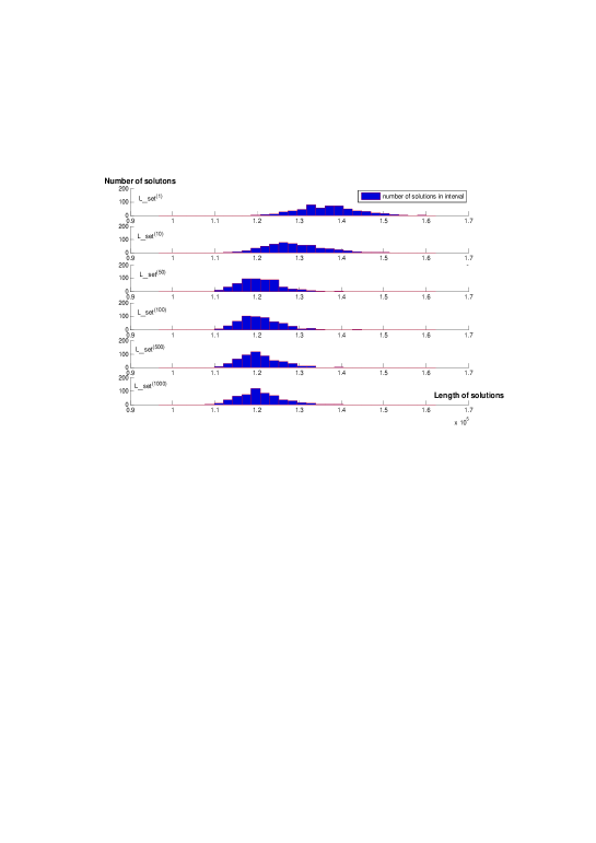
Figure 2: The Histogram of the Route Length Set $L\_Set^{(t)}$: $X-axis$ represents the value of route length $x$, $Y-axis$ represents the probability that the routes with length $x$ being selected by ants . In this figure, the probability is replaced by frequency for direct-viewing. This figure shows that set $L\_Set^{(t)}$ has statistical feature. The distribution of set $L\_Set^{(t)}$ is convergent. Notice: The test data is pr136,  number of cities and ants is 136 and 544 respectively. The $x-axis$ is divided into equal interval with size 2183 (i.e.$\delta=2183$ ). The histogram of at $t-th$ iteration is shown here, where $t=1,10,50,100,500,1000$. The same features are also found in other test data, such as pr107, d198, pr226, d493 and so on. All test data in this paper is downloaded from http://www.iwr.uniheidelberg.de/iwr/comopt/soft/TSPLIB95/TSPLIB.html

III.3 The Expectation and Deviation of Route Length Set

Expectation and deviation are the two most essential characteristics of distribution, these two characteristics of set $L\_Set^{(t)}$ will be calculated in this section. The expectation and standard deviation of set $L\_Set^{(t)}$ are denoted by $\overset{-}{L}^{(t)}$and $\sigma^{(t)}$ respectively in this paper. $\overset{-}{L}$ and $\sigma^{(t)}$ are defined as below:

Definition 4 (the expectation of set $L\_Set^{(t)}$):

$$\overset{-}{L}^{(t)}=\frac{1}{m}\overset{m}{\underset{i=1}{\sum L_{i}^{(t)}}}$$ (7)

, where $m$ is the number of ants.

Definition 5 (the standard deviation of set $L\_Set^{(t)}$):

$$\sigma^{(t)}=\sqrt{\frac{1}{m}\overset{m}{\underset{i=1}{\sum}}|L_{i}^{(t)}-\overset{-}{L}^{(t)}|^{2}}$$ (8)

Two sequences $\{\overset{-}{L}^{(1)},\overset{-}{L}^{(2)},...,\overset{-}{L}^{(t)},...\}$ and $\{\sigma^{(1)},\sigma^{(2)},...,\sigma^{(t)},...\}$ are shown at Fig.3. The subfigure (a) of Fig.3 shows that expectation $\overset{-}{L}^{(t)}$descends continuously and converges to a constant value. The subfigure (b) shows that all standard deviations fluctuate narrowly in an interval and most of deviations are close to a constant value.

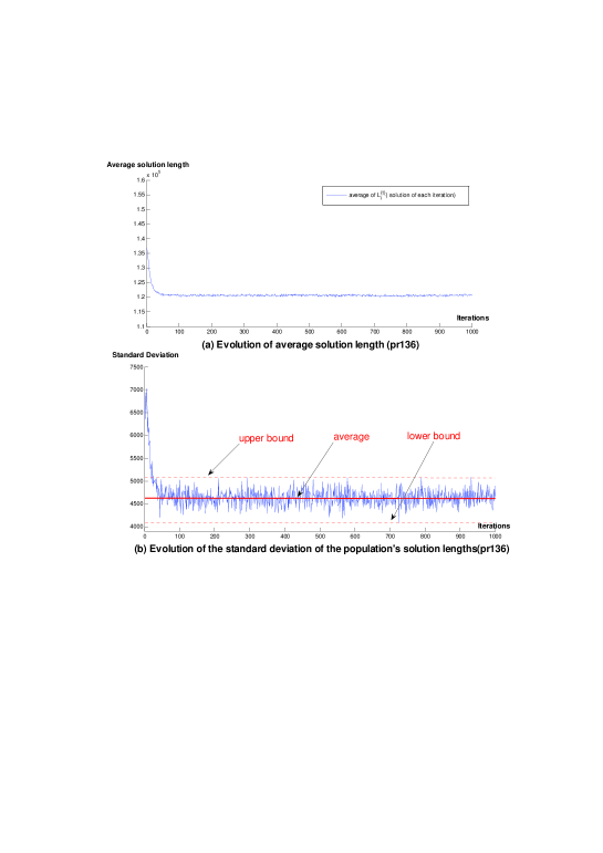
Figure 3: The Feature of Expectation and Standard Deviation of Route Length Set: Figure (a) and (b) diagrammatize the two curves of sequence $\{\overset{-}{L}^{(1)},\overset{-}{L}^{(2)},...,\overset{-}{L}^{(t)},...\}$ and $\{\sigma^{(1)},\sigma^{(2)},...,\sigma^{(t)},...\}$ respectively, where $\overset{-}{L}^{(t)}$and $\sigma^{(t)}$ are the expectation and standard deviation of route length set $L\_Set^{(t)}$ respectively. Figure (a) shows that expectation descends continuously and converges to a constant value. Figure (b) shows that all standard deviations fluctuate narrowly in a small interval comparing with average route length and most of deviations are close to a constant value. The similar feature are observed from other instances, such as pr107, d198, pr226, d493 and so on. Notice: The test data in this figure is pr136, the number of cities is $n=136$, the number of ants is $m=544$, and the number of maximum iteration is $N_{C_{\max}}=1000$.

III.4 Holding View Point of Statistics to Understand ACO Convergence

There are three types of understanding for the convergence of ACO:

Type 1: With the increase of iteration steps, all ants will select the optimal route which has shortest length.

Type 2: With the increase of iteration steps, all ants will select a unique fixed (or stable) route, but it is not optimal possibly.

Type 3: With the increase of iteration steps, more than one fixed routes are selected by different ants. That is, ACO converges to a stable set which consists of some fixed routes, not a unique route.

ACO converging to optimal route is difficult in general, the first type is not common in practice. The 2nd type is also not common in practice, and it never be observed in the authors’ experiment. Instead of the 2nd type, the 3rd type is common in practice. For example, Fig.2 shows that, there are always different routes selected by ants at every iteration step, and the convergent route is not unique. Since the 3rd type is common and has more practical worthiness, the convergence of ACO refers to this type in this paper.

In addition, the aim of ACO is to find the shortest route length, and the difference of the routes is not cared. Therefore, a equivalent statement of the 3rd type is that, ACO converges to a stable set which consists of stable route lengths .

According to above discusion, if ACO converges, the stable set will appear, which consists of stable route lengths. Then the histogram of this stable set is convergent (see Fig. 2). That is, ACO converging results in probability sequence $\{h_{1}(x),h_{2}(x),...,h_{t}(x),...\}$ being convergent. At the same time, sequence $\{h_{1}(x),h_{2}(x),...,h_{t}(x),...\}$ being convergent will result in ACO converging also, and it is proved as below:

Let set $A_{t}(x)=\{j|L_{j}^{(t)}=x\}$. Then $h_{t}(x)=\frac{|A_{t}(x)|}{m}$. Thus, if $\{h_{1}(x),h_{2}(x),...,h_{t}(x),...\}$ is convergent, $|A_{t}(x)|$ becomes fixed (or stable). Since route $r_{j}^{(t)}$ represents the route selected by ant $a_{j}$, number $|A_{t}(x)|$ represents the number of ants which routes has length $x$. There are only two factors to cause $|A_{t}(x)|$ becoming fixed. One factor is ACO being convergent. The other factor is that, some ants coming into set $A_{t}(x)$ and some coming out, the quantities of input and output are equal. The second factor is too special so that it does not exist. Therefore, if $\{h_{1}(x),h_{2}(x),...,h_{t}(x),...\}$ is convergent, ACO will be convergent.

According to above discussion, the following conclusion is obtained:

Conclusion 1: ACO being convergent is equivalent to the sequence of probability functions $\{h_{1}(x),h_{2}(x),...,h_{t}(x),...\}$ being convergent.

This conclusion shows that, the histogram of route length set becoming convergent is the marker of ACO being convergent (see Fig.2).

IV Using Pheromone Probability to Observe The Statistical Feature of Route Length Set

IV.1 The Pseudo-Probability and Pseudo-Histogram of Route Length Set

The definition of pseudo-probability $h_{t}^{{}^{\prime}}(x)$:

At the $t-th$ iteration step, every ant will select a route. The $i-th$ ant $a_{i}$ selects route $r_{i}^{(t)}$, and $r_{i}^{(t)}$ has length $L_{i}^{(t)}$, where $i=1,2,...,m$. Each route $r_{i}^{(t)}$ contains the amount of pheromone $f_{i}^{(t)}$, which is the sum of pheromone depositing on every edge of route $r_{i}^{(t)}$. The pheromone probability is the ratio of pheromone, it is defined as $p_{i}^{(t)}=\frac{\ f_{i}^{(t)}}{\overset{m}{\underset{j=1}{\sum}}f_{j}^{(t)}}$.

Set $A_{t}(x)=\{j|L_{j}^{(t)}=x\}$ is the subscripts set of routes which length is a given value $x$. Basing on set $A_{t}(x)$, pseudo-probability is defined as

$$h_{t}^{{}^{\prime}}(x) = \underset{j\in A_{t}(x)}{\sum p_{j}^{(t)}}$$

$$x \in [L_{inf},L_{sup}]$$

, where $L_{inf}=min\{L_{i}^{(t)}\}$ and $L_{sup}=max\{L_{i}^{(t)}\}$.

Pseudo-probability $h_{t}^{{}^{\prime}}(x)$ is the sum of pheromone probabilities which associated route has length $x$.

The pseudo-histogram of route length set $L\_Set^{(t)}$:

Pseudo-histogram is also a histogram in which pseudo-probability $h_{t}^{{}^{\prime}}(x)$ replace probability $h_{t}(x)$ to estimate the distribution of route length set $L\_Set^{(t)}$. It is generated by following method:

Firstly, a two-dimensional coordinate frame is constructed, the $x-axis$ denotes the value of route length $x$, and the $y-axis$ denotes pseudo-probability $h_{t}^{{}^{\prime}}(x)$. The $x-axis$ is divided into equal intervals, and the size of each interval is denoted by $\delta$.

Secondly, calculate the approximation of pseudo-probability for every interval $I$: Suppose $x$ represents argument and $x\in I$. A counter $d$ is attached to interval $I$, and its initial value is set to zero (i.e., $d=0$;). If $L_{i}^{(t)}$ falls into interval $I$ (i.e., $L_{i}^{(t)}\in I$), its associated pheromone probability $p_{i}^{(t)}$ is add to $d$ (i.e., $d=d+p_{i}^{(t)}$). The value $d$ is the function value of argument $x$. When the size of interval $I$ limits to zero ideally, the value $d$ limits to pseudo-probability $h_{t}^{{}^{\prime}}(x)$.

The pseudo-histogram is shown in Fig.4. Comparing with the histogram of probability function shown at Fig.2, pseudo-histogram is very similar to it. Probability $h_{t}(x)$ represents the degree of possibility that the routes with length $x$ being selected by ants, pseudo-probability $h_{t}^{{}^{\prime}}(x)$ represents the sum of pheromone probability $p_{i}^{(t)}$ which associated route $r_{i}^{(t)}$ has length $x$. The similarity of these two figures excites the guess that pseudo-probability is the approximation of probability(i.e., $h_{t}(x)\thickapprox h_{t}^{{}^{\prime}}(x)$).

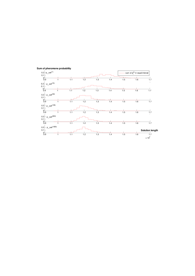
Figure 4: The Pseudo-Histogram of Route Length Set $L\_Set^{(t)}$ Calculated by Pheromone Probability $p_{i}^{(t)}$. The $X-axis$ denotes the value of route length $x$ and is divided into small intervals. The value at $Y-axis$ denotes the pseudo-probability $h_{t}^{{}^{\prime}}(x)$, which is the sum of all pheromone probabilities $p_{i}^{(t)}$ under the condition $L_{i}^{(t)}=x$. The input data of this instance is pr136, where the number of cities $n=136$, number of ants $m=544$ and length of interval $\delta=2183$. Comparing with Figure.2, this figure is similar to it. And this similarity excites the guess pseudo-probability $h_{t}^{{}^{\prime}}(x)$ is the approximation of probability $h_{t}(x)$, which represents the degree of possibility that the routes with length $x$ being selected by ants.

IV.2 Pseudo-Expectation $\overset{-}{L}^{{}^{\prime}(t)}$and Pseudo-Deviation $\sigma^{{}^{\prime}(t)}$

Definition 6 ($\overset{-}{L}^{{}^{\prime}(t)}$, Pseudo-Expectation of Route Length Set $L\_Set^{(t)}$ Calculated by Pheromone Probability):

$$\overset{-}{L}^{{}^{\prime}(t)}=\underset{x\in V}{\sum}xh_{t}^{{}^{\prime}}(x)=\overset{m}{\underset{i=1}{\sum}}L_{i}^{(t)}\times p_{i}^{(t)}$$ (9)

, where $x$ denotes the value of route length and $V$ denotes the set of these values.

Definition 7 ($\sigma^{{}^{\prime}(t)}$, Pseudo-Deviation Calculated by Pheromone Probability):

$$\sigma^{{}^{\prime}(t)}=\sqrt{\overset{m}{\underset{i=1}{\sum}p_{i}^{(t)}}|L_{i}^{(t)}-\overset{-}{L}^{{}^{\prime}(t)}|^{2}}$$ (10)

The two sequence {$\overset{-}{L}^{{}^{\prime}(1)},\overset{-}{L}^{{}^{\prime}(2)},...,\overset{-}{L}^{{}^{\prime}(t)},...$} and sequence {$\sigma^{{}^{\prime}(1)},\sigma^{{}^{\prime}(2)},..,\sigma^{{}^{\prime}(t)},...$} are shown at Fig.5. Comparing with Fig.3, Fig.5 is very similar to it. Two sequences {$|\overset{-}{L}^{(t)}-\overset{-}{L}^{{}^{\prime}(t)}|$} and {$|\sigma^{(t)}-\sigma^{{}^{\prime}(t)}|$} are shown in Fig.6, this figure demonstrates that $\overset{-}{L}^{(t)}\thickapprox\overset{-}{L}^{{}^{\prime}(t)}$and $\sigma^{(t)}\thickapprox\sigma^{{}^{\prime}(t)}$. Expectation and deviation are two most important characteristics of set of random data. And Fig.5 and Fig.6 are two evidences to support the conclusion

$$h_{t}(x)\thickapprox h_{t}^{{}^{\prime}}(x)$$

, where $h_{t}(x)$ and $h_{t}^{{}^{\prime}}(x)$ denotes the probability and pseudo-probability respectively.

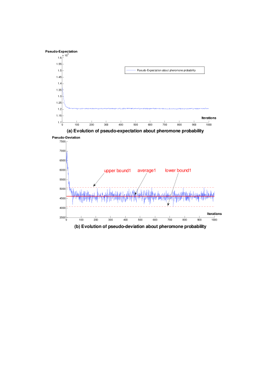
Figure 5: Pseudo-Expectation $\overset{-}{L}^{{}^{\prime}(t)}$and Pseudo-Deviation $\sigma^{{}^{\prime}(t)}$ : Comparing with Fig.3, this figure is similar to it. This similarity provides a evidence to support conclusion 2: $h_{t}(x)\thickapprox h_{t}^{{}^{\prime}}(x)$. Notice: The input data of this shown instance is pr136, the number of ants $m=544$, the number of cities $n=136$ and the number of maximum iteration $N_{C_{\max}}=1000$. The same conclusion is also found in other test data, such as pr107, d198, pr226, d493 and so on.

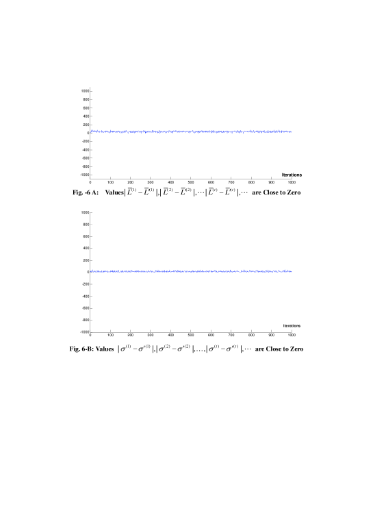
Figure 6: Sequence of Pesudo-Expectation $\{\overset{-}{L}^{{}^{\prime}(t)}\}$ and Pesudo-Deviation $\{\overset{-}{\sigma}^{{}^{\prime}(t)}\}$ Is Close to $\overset{-}{\{L}^{(t)}\}$ and $\{\overset{-}{\sigma}^{(t)}\}$ Respectively. Two sequences {$|\overset{-}{L}^{(t)}-\overset{-}{L}^{{}^{\prime}(t)}|$} and {$|\sigma^{(t)}-\sigma^{{}^{\prime}(t)}|$} are shown in this figure. This figure shows that $\overset{-}{L}^{(t)}\thickapprox\overset{-}{L}^{{}^{\prime}(t)}$and $\sigma^{(t)}\thickapprox\sigma^{{}^{\prime}(t)}$. This evidence further supports conclusion 2. Notice: The experiment parameters are same to Fig.5

Since histogram and pseudo-histogram is very similar and $\overset{-}{L}^{(t)}\thickapprox\overset{-}{L}^{{}^{\prime}(t)}$and $\sigma^{(t)}\thickapprox\sigma^{{}^{\prime}(t)}$, we have following conclusion:

Conclusion 2: With the increasing of iteration step, pseudo-probability is the approximation of probability (i.e., $h_{t}(x)\thickapprox h_{t}^{{}^{\prime}}(x)$ when $t\rightarrow\infty$).

Conclusion 1 shows probability function $h_{t}(x)$ being convergent is equivalent to ACO being convergent. Since $h_{t}(x)\thickapprox h_{t}^{{}^{\prime}}(x)$, we have

Conclusion 3: Pseudo-probability $h_{t}^{{}^{\prime}}(x)$ being convergent is equivalent to ACO being convergent

Pseudo-probability $h_{t}^{{}^{\prime}}(x)$ being convergent results in ACO being convergent. And when ACO being convergent, every route selected by ant is fixed. This situation results in the amount of pheromone depositing on convergent route is fixed and its ratio (i.e., pheromone probability $p_{i}^{(t)}$) is fixed too. Therefore, function $h_{t}^{{}^{\prime}}(x)$ being convergent results in pheromone probability $p_{i}^{(t)}$ being convergent, where $i=1,2,...,m$. On the other hand, pheromone probability $p_{i}^{(t)}$ being convergent results in the function $h_{t}^{{}^{\prime}}(x)$ being convergent and ACO being convergent. Then, we have

Conclusion 4: Pseudo-probability $h_{t}^{{}^{\prime}}(x)$ being convergent is equivalent to pheromone probability set $P\_Set^{(t)}$ being convergent, where the convergence of $P\_Set^{(t)}$ refers to that every pheromone probability in this set is convergent.

Conclusion 5: Pheromone probability set $P\_Set^{(t)}$ being convergent is equivalent to ACO being convergent.

V Entropy Convergence

V.1 Entropy of Pheromone and Its Convergence

In 1948 Shannon introduced the entropy Shannon into information theory for the first time. In information theory, entropy is a measure of the uncertainty associated with random system. The lower entropy is, the lower the uncertainty of system is. Entropy is defined as

$$H=-\overset{n}{\underset{i=1}{\sum}}p_{i}\cdot log_{{}_{2}}p_{i}$$ (11)

, where $p_{i}$ denotes the probability.

At $t-th$ iteration of ACO, ant $a_{i}$ select route $r_{i}^{(t)}$, where $i=1,2,...,m$. Route $r_{i}^{(t)}$ associates with pheromone probability $p_{i}^{(t)}$, which is the ratio of pheromone assigned at route $r_{i}^{(t)}$. All pheromone probability $p_{i}^{(t)}$ comprise set $P\_Set^{(t)}=\{p_{1}^{(t)},p_{2}^{(t)},...,p_{i}^{(t)},...,p_{m}^{(t)}\}$.

According to Eq.11, entropy of pheromone is defined as

$$H(P\_Set^{(t)})=-\overset{n}{\underset{i=1}{\sum}}p_{i}^{(t)}\cdot log_{{}_{2}}p_{i}^{(t)}$$ (12)

It is simplified as

$$H_{t}=-\overset{n}{\underset{i=1}{\sum}}p_{i}^{(t)}\cdot log_{{}_{2}}p_{i}^{(t)}$$ (13)

Pheromone probability $p_{i}^{(t)}$ represents the ratio of pheromone assigned at route $r_{i}^{(t)}$. If every route is assigned equal amount of pheromone, all ants don’t know which route is best and select route randomly. At this time, all pheromone probabilities are equal (i.e., $p_{i}^{(t)}=\frac{1}{m}$), entropy of pheromone is maximum, and the uncertainty degree that ants selecting route is maximum. And this situation is often happened at the early iteration steps of ACO. If pheromone is assigned at few routes, most of ants will select these routes with high probability. At this time, there is low uncertainty for ants selecting route, entropy is small. This situation is often happened at the iteration steps at which ACO is close to convergence.

With the increase of iteration step, every route selected by ants will become fixed, the pheromone depositing on it becomes fixed (stable) and its pheromone probability becoming fixed too. This situation results in the sequence $\{H_{1},H_{2},...,H_{t},...\}$ converging. The test result at Fig.7 shows that the entropy sequence is convergent.

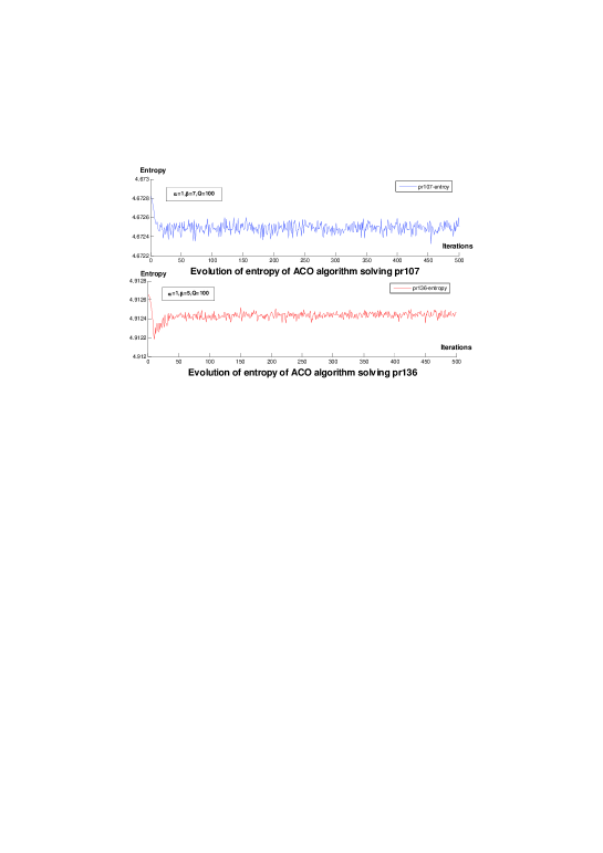
Figure 7: Entropy of Pheromone Is Convergent. Two curves show that two entropy sequences are convergent approximately. And the amplitude of swing is very narrow, it is less than $0.0002/4.6$ or $0.0004/4.9$ . Notice: The shown test data are pr107 and pr136, the number of ant is equal to the number of cites (i.e. $m=107$ and $m=136$), the number of maximum iteration is $N_{C_{\max}}=500$ and the feature of entropy convergence is observed from other test data also, such as d198, pr226, d493 and so on. The entropy is calculated by $H(t)=-\overset{n}{\underset{i=1}{\sum}}p_{i}^{(t)}\cdot lnp_{i}^{(t)}$ in this figure.

V.2 Entropy Convergence Is A Marker of ACO Convergence

Entropy is the most essential characteristics of a random system. Thus, the convergence of entropy sequence $\{H_{1},H_{2},...,H_{t},...\}$ is the marker of the convergence of set $P\_Set^{(t)}$. Set $P\_Set^{(t)}$ being convergent is equivalent to ACO being convergent according to conclusion 5. Therefore, the convergence of entropy sequence $\{H_{1},H_{2},...,H_{t},...\}$ is the marker of the convergence of ACO. When ACO is convergent, set $P\_Set^{(t)}$ is convergent, entropy sequence is convergent too. If ACO is not convergent, set $P\_Set^{(t)}$ is not convergent, entropy sequence is not convergent too. On the other hand, when entropy sequence is convergent, set $P\_Set^{(t)}$ is convergent very possibly because entropy is its essential characteristic, ACO is convergent too. If entropy sequence is not convergent, set $P\_Set^{(t)}$ is not convergent very possibly, ACO is not convergent too.

Therefore, the convergence of entropy sequence is a marker of minimum iteration steps at which ACO is convergent.

In addition, the convergence of entropy sequence $\{H_{1},H_{2},...,H_{t},...\}$ has usual  criterion $\frac{|H_{t}-H_{t-1}|}{H_{t-1}}<\varepsilon$ Pang . And criterion$\frac{|H_{t}-H_{t-1}|}{H_{t-1}}<\varepsilon$ is a very simple criterion to estimate the minimum iteration number at which ACO is convergent possibly.

VI Application of Entropy Convergence

VI.1 Apply Entropy Convergence as Termination Criterion of ACO

The improved ACO algorithm with criterion $\frac{|H_{t}-H_{t-1}|}{H_{t-1}}<\varepsilon$ is presented as below, and it is named ACO-Entropy in this paper.

Algorithm ACO-Entropy

Step1. Initialize pheromone trails for all edges and put $m$ ants at different cities. Let $t=0$ , $\Delta\tau_{ij}(0)=0$ and $H_{0}=\log_{2}m$.

Step2. do

{

Step2.1 $t\leftarrow t+1$.

Step2.2 The ants choose next cities according to transition probability.

Step2.3 After all ants finish their travels, pheromone are updated.

Step2.4 The pheromone probability $p_{i}^{(t)}$ and the entropy $H_{t}$ are calculated by

formula  (6) and (13) respectively.

}while($\frac{|H_{t}-H_{t-1}|}{H_{t-1}}\geq\varepsilon$)

Step3. End procedure and output result.

VI.2 The Experiment and Comparison

All data tested in this paper are downloaded from http://www.iwr.uniheidelberg.de/iwr/

comopt/soft/TSPLIB95/TSPLIB.html. All algorithms in this paper run on personal computer, CPU (2): 1.60GHZ, Memory: 480M, Software: Matlab 7.1. All parameters are set as below:

$\alpha=1$, $\beta=8$, $\rho=0.4$, $Q=100$, $\tau_{ij}(0)=1$, $m=n$, $\varepsilon=0.001$, $N_{C_{\max}}=1000$.

To test the performance of ACO-Entropy, two algorithms of ACO and the ACO-Entropy are tested in this paper, where ACO refers to Ant-Cycle shown at section II, which is often used standard algorithm.

Table.1 and Fig.8 show that, ACO-Entropy is faster than ACO by factors of 2-6 under the same condition and nearly same quality of solution is obtained.

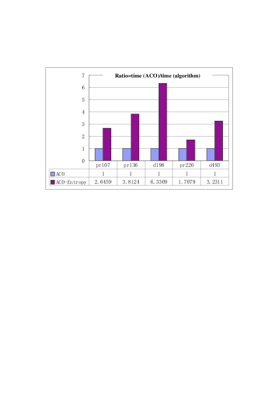
Figure 8: Comparison of the Running Speed of ACO and ACO-Entropy. ACO-Entropy is faster than ACO by factors of 2-6 under the same condition and the nearly same quality of solution is obtained (see Table 1), where ACO refers to Ant-Cycle shown at section II.

Input	Number	ACO-Entropy
Data	of Test	Average Solution	Average Time(s)	Iteration Number
pr107	10	46294	163.0804	189
pr136	10	108467	173.3620	131
d198	10	17135	447.4071	100
pr226	10	84718	2466.1	293
d493	2	39851	16405	155
		ACO
pr107	10	45973	431.496	500
pr136	10	102608	660.918	500
d198	10	16891	2832.5	500
pr226	10	84514	4211.8	500
d493	2	38926	53007	200
Table1. Performance Comparison of ACO and ACO-Entropy: This table shows that ACO-Entropy is faster than ACO by factors of 2-6. The two solution qualities of ACO-Entropy and ACO are nearly same.

VII Conclusion

The convergence of ACO is the base of ACO, its study is not much currently. The convergence under some special conditions has be studied, and the view point of study are Graph theory, Markov process, and so on. It is interesting to find a new view point to study ACO convergence under general condition. The aim of this paper is to explore new view point of studying ACO convergence under general condition and to find the new marker of ACO convergence.

Since ACO is kind of probabilistic algorithm, the feature of its convergence possibly hide in some statistical properties. Thus, the analysis of statistical property is the start point of study of this paper. Along this start point, five equivalent statements of ACO convergence are found in this paper (see Conlusion 1-5). And these equivalent statements result in the following conclusion:

ACO may not converges to the optimal solution in practice, but its entropy is convergent under general condition.

- (1) M. Dorigo, V. Maniezzo, and A. Colorni. Positive feedback as a search strategy. Technical Report 91-016, Dipartimento di Elettronica, Politecnico di Milano, Milan, Italy, 1991.
- (2) A. Colorni, M. Dorigo, and V. Maniezzo. Distributed Optimization by Ant Colonies. In F. J. Varela and P. Bourgine, editors, Towards a Practice of Autonomous Systems: Proceedings of the First European Conference on Artificial Life, pages 134-142. MIT Press, Cambridge, MA, 1992.
- (3) M. Dorigo. Optimization, Learning and Natural Algorithms. PhD thesis, Dipartimento di Elettronica, Politecnico di Milano, Milan, Italy, 1992.
- (4) M. Dorigo and L. M. Gambardella. Ant Colony System: A Cooperative Learning Approach to the Traveling Salesman Problem. IEEE Transactions on Evolutionary Computation, 1(1):53-66, 1997.
- (5) L. M. Gambardella and M. Dorigo. Solving Symmetric and Asymmetric TSPs by Ant Colonies. In T. Baeck, T. Fukuda, and Z. Michalewicz, editors, IEEE International Conference on Evolutionary Computation - CEC’96, pages 622-627. IEEE Press, Piscataway, NJ, 1996.
- (6) M. Dorigo and G. Di Caro. The Ant Colony Optimization Meta-Heuristic. In D. Corne, M. Dorigo, and F. Glover, editors, New Ideas in Optimization, chapter 2, pages 11-32. McGraw-Hill, London, UK, 1999.
- (7) M. Dorigo, G. Di Caro, and L. M. Gambardella. Ant Algorithms for Discrete Optimization. Artificial Life, 5(2):137-172, 1999.
- (8) S. Kirkpatrick, C. D. Gelatt, and M. P. Vecchi, Optimization by Simulated Annealing, Science, Volume 220,Number 4598 pp. 671–680, 1983.[online] http://info.ruc.edu.cn/wangqiuyue/lec-notes/comp_en/ 1983-Optimization%20by%20simulated%20annealing.pdf
- (9) Fred Glover , Fred Laguna, Tabu Search, Kluwer Academic Publishers, Norwell, MA, 1997.
- (10) David E. Goldberg, Genetic Algorithms in Search, Optimization and Machine Learning, 1st edition, Addison-Wesley Longman Publishing Co., Inc. Boston, MA, USA , 1989.
- (11) M.O. Ball, T.L. Magnanti, C.L. Monma, and G.L. Nemhauser, HANDBOOKS IN OPERATIONS RESEARCH AND MANAGEMENT SCIENCE, 7: NETWORK MODELS, North Holland, 1995.
- (12) M.O. Ball, T.L. Magnanti, C.L. Monma, and G.L. Nemhauser,HANDBOOKS IN OPERATIONS RESEARCH AND MANAGEMENT SCIENCE, 8: NETWORK ROUTING, North Holland, 1995.
- (13) L. M. Gambardella and M. Dorigo. Ant-Q: A Reinforcement Learning Approach to the Traveling Salesman Problem. In A. Prieditis and S. Russell, editors, Machine Learning: Proceedings of the Twelfth International Conference on Machine Learning, pages 252-260. Morgan Kaufmann Publishers, San Francisco, CA, 1995.
- (14) L. M. Gambardella, ? D. Taillard, and M. Dorigo. Ant Colonies for the Quadratic Assignment Problem. Journal of the Operational Research Society, 50(2):167-176, 1999.
- (15) B. Bullnheimer, R. F. Hartl, and C. Strauss. Applying the ant system to the vehicle routing problem, IN I. H. Osman, S. Vo, S. Martello and C. Roucairol, editors, Meta-Heuristics: Advances and Trends in Local Search Paradigms for Optimization, pages 109-120. Kluwer Academics, 1998.
- (16) P. Forsyth and A. Wren. An ant systemfor bus driver scheduling. Technical Report 97.25, University of Leeds , School of Computer Studies , July 1997. Presented at the 7th International Workshop on Computer - Aided Scheduling of Public Transport , Boston , July 1997.
- (17) Rafael S. Parpinelli, Heitor S. Lopes, “Data Mining With an Ant Colony Optimization Algorithm,” IEEE Transactions on Evolutionary Computation, vol. 6, no. 4, pp. 321-332, 2002.
- (18) W. J. Gutjahr ACO algorithms with guaranteed convergence to the optimal solution. Information Processing Letters, 2002, 82(3): 145-153
- (19) T. Stezle and M. Dorigo. A Short Convergence Proof for a Class of ACO Algorithms. IEEE Transactions on Evolutionary Computation, 6(4):358-365, 2002.
- (20) J.-H. Yoo, R. J. La, and A.M. Makowski, Convergence Results for Ant Routing, Proc. Conf. on Inf. Sc. and Systems, Princeton, NJ, 2004.
- (21) J.-H. Yoo, R. J. La and A. M. Makowski, Convergence of ant routing algorithms – Results for a simple parallel network and perspectives, Technical Report CSHCN 2003-44, Institute for Systems Research, University of Maryland, College Park (MD), 2003.
- (22) Sun Tao and Wang Xiu kun,et al. Ant Algorithm and Analysis on its Convergence. Mini-micro Systems, 2003, 21(8): 1524–1526.
- (23) Ding Jian li, Chen Zeng qing and Yuan Zhu zhi. On the Markov Convergence Analysis for the Combination of Genetic Algorithm and Ant Algorithm. Acta Automatia Sinica, 2004, 30(4): 659–664
- (24) Y. H. Hou , Y. W. Wu, L. J. Lu, et al. Generalized ant colony optimization for economic dispatch of power systems . Proceedings of the 2002 International Conference on Power System Technology, Vol 1. 2002. pp.225-229
- (25) C. E. SHANNON, A Mathematical Theory of Communication, Reprinted with corrections from The Bell System Technical Journal,Vol. 27, pp. 379-423, 623-656, July, October, 1948. [online] http://cm.bell-labs.com/cm/ms/what/shannonday/shannon1948.pdf
- (26) Chao-Yang Pang. Vector Quantization and Image Compression. Ph.D. Thesis, University of Electronic Science and Technology of China, Chengdu, China, Jun 2002.