MPP-2009-40

May 2009

The puzzle of apparent linear lattice artifacts in the 2d non-linear $\sigma$–model and Symanzik’s solution

Janos Balog

Research Institute for Particle and Nuclear Physics

1525 Budapest 114, Pf. 49, Hungary

Ferenc Niedermayer

Institute for Theoretical Physics, University of Bern

CH-3012 Bern, Switzerland

Peter Weisz

Max-Planck-Institut für Physik

Föhringer Ring 6, D-80805 München, Germany

Abstract

Lattice artifacts in the 2d O($n$) non-linear $\sigma$–model are expected to be of the form ${\rm O}(a^{2})$, and hence it was (when first observed) disturbing that some quantities in the O(3) model with various actions show parametrically stronger cutoff dependence, apparently ${\rm O}(a)$, up to very large correlation lengths. In a previous letter [?] we described the solution to this puzzle. Based on the conventional framework of Symanzik’s effective action, we showed that there are logarithmic corrections to the ${\rm O}(a^{2})$ artifacts which are especially large ($\ln^{3}a$) for $n=3$ and that such artifacts are consistent with the data. In this paper we supply the technical details of this computation. Results of Monte Carlo simulations using various lattice actions for O$(3)$ and O$(4)$ are also presented.

1 Introduction

In a previous letter [?] we presented results on logarithmic corrections to ${\rm O}(a^{2})$ lattice artifacts for a class of lattice actions for the non-linear ${\rm O}(n)$ sigma-model in two dimensions. It is the purpose of this paper to supply the technical details of the computation. The main results, which are summarized in subsection 3.5, are that the generic leading artifacts are of the form $a^{2}\left[\ln(a^{2})\right]^{n/(n-2)}$, and this result together with the next-to-leading expressions describe well the lattice artifacts in the step scaling function [?], which are for $n=3$ in a large range of the cutoff apparently of the form ${\rm O}(a)$ [?]. The goal of our work was indeed to explain this long-standing scientific puzzle which was mentioned by Hasenfratz in his lattice plenary talk in 2001 [?].

Most of our knowledge concerning renormalization of quantum field theories stems from perturbation theory. Although there are no rigorous proofs in general, many of the results are structural and hence considered to carry over to non-perturbative formulations. Indeed there is supporting evidence from various studies, e.g. of soluble models in 2 dimensions and of $1/n$ expansions of some theories. The same situation holds concerning cutoff artifacts in lattice regularized theories.

Thus we start our paper with perturbative considerations. In section 2 we briefly summarize perturbative renormalization of the sigma model in the framework of dimensional regularization, including the renormalization of isoscalar composite operators of dimension 4. Next we discuss a large class of lattice regularizations. We summarize the results for connected 2– and 4–point functions to 1-loop order and also the relations of the corresponding renormalized functions to those of the dimensionally regularized theory.

In the early 80’s Symanzik was working on the nature of lattice artifacts, in particular with respect to his improvement program [?,?,?,?,?]. In this paper the general theory is not discussed; we only consider in section 3 Symanzik’s theory applied to the 2-dimensional O$(n)$ $\sigma$-model. Nevertheless the spirit of the general theory can already be understood by studying this example. Symanzik’s main conclusion is that leading artifacts are summarized in an effective action.

In this framework generic lattice artifacts are, in particular for asymptotically free (or trivial) theories, expected to be integer powers in the lattice spacing ${\rm O}(a^{p})\,,p=1,2,\dots$ up to possible multiplicative logarithmic corrections. In particular this framework explains why in the 2-dimensional $\sigma$-model quadratic artifacts are expected. To obtain the effective action in lowest orders of perturbation theory we compute the leading lattice artifacts in the 2- and 4-point functions to 1-loop order and express them in terms of insertions of composite operators of dimension 4 in the continuum. This is a rather lengthy computation and thus many technical details are relegated to the Appendices.

In section 4 we reanalyze the presently available Monte Carlo data on the step scaling function for cases $n=3$ and $n=4$. In particular for the case $n=3$ we study three different lattice actions, and see how the particular logarithmic corrections predicted by Symanzik’s theory solves the puzzle of apparent linear artifacts. Similar conclusions that logarithmic corrections may explain the puzzle have been reached previously in studies of the ${\rm O}(n)$ model in the first orders of the $1/n$ expansion [?,?,?]. In Appendix E we describe a modified version of Hasenbusch’s improved estimator which was essential to obtain a sufficiently small error for small $a/L$ values.

There is a vast literature on the subject of this paper, however we feel that this technical report is not the appropriate place to properly review all important contributions. Hence we restrict ourselves here to citing a selection of papers where the reader can find further references. 2-dimensional O$(n)$ spin systems, including the Ising model and the large $n$ limit, are reviewed in [?]. Various aspects (on the lattice and in the continuum) of the exactly solvable $n\to\infty$ limit, using a number of different lattice actions, are reviewed in [?]. Symanzik’s improvement program for the 2-dimensional O$(n)$ models are studied in [?,?] and some exact results about the lattice artifacts in the large $n$ limit are given in [?].

2 The non-linear O($n$) sigma model in two dimensions

The non-linear O($n$) sigma model describes the interaction of spin fields $S^{a}(x)\,,a=1,\dots,n$ with the constraint $S(x)^{2}=1$ in two space-time dimensions. Here we consider the space-time to be Euclidean. Formally the Lagrangian is that of a free massless field and the interaction derives entirely from the constraint. The field theory requires an ultra-violet regularization; in the next subsection we will consider dimensional regularization and then in subsect. 2.2 a class of lattice regularizations.

2.1 Dimensional regularization

The action of the O$(n)$ model in $D=2-\varepsilon$ dimensions (including source terms) is

$${\cal A}=\frac{1}{g_{0}^{2}}\int{\rm d}^{D}x\,\left\{\frac{1}{2}\partial_{\mu}S\cdot\partial_{\mu}S-I\cdot S\right\}\,,$$ (2.1)

where $g_{0}$ is the bare coupling. To satisfy the constraint it is usual to parameterize the bare spin field by

$$S^{i}=g_{0}\pi^{i},\qquad i=1,2,\dots,n-1;\qquad\qquad S^{n}=\sigma=\sqrt{1-g_{0}^{2}\pi^{2}}\,.$$ (2.2)

The source dependent action (2.1) appears in the generating functional

$${\cal Z}[I]=\int\left({\cal D}\pi\right)\,{\rm e}^{-{\cal A}}\,,$$ (2.3)

which can be used to obtain bare correlation functions of the field $S^{a}(x)$ using the formula

$${\cal G}^{a_{1}\dots a_{r}}(x_{1},\dots,x_{r})=g_{0}^{2r}{\cal Z}^{-1}[I_{0}]\frac{\delta}{\delta I^{a_{1}}(x_{1})}\dots\frac{\delta}{\delta I^{a_{r}}(x_{r})}\Big{|}_{I_{0}}\,{\cal Z}[I]\,,$$ (2.4)

where the functional derivative is taken at

$$I^{a}_{0}(x)=m^{2}\delta^{an}\,,$$ (2.5)

i.e. a mass term (external magnetic field) is introduced to avoid infrared singularities. As proven by David [?], O($n$) invariant correlators are infrared finite order by order in perturbation theory and hence for these the limit $m\to 0$ can be taken at the end of the calculation.

In their seminal paper [?] Brézin, Zinn-Justin and Le Guillou prove the renormalizability of the O$(n)$ model using functional methods. In this paper they show that the generating functional ${\cal Z}^{-1}[I_{0}]{\cal Z}[I]$ is finite as function of the renormalized quantities $j^{a}(x),g,\mu,m_{R}$ if we write

$$\begin{split}I^{a}(x)&=Z_{1}(g,\varepsilon)Z^{-1/2}(g,\varepsilon)g^{2}j^{a}(x)+I^{a}_{0},\\ g_{0}^{2}&=\mu^{\varepsilon}Z_{1}(g,\varepsilon)g^{2}\,,\\ m^{2}&=Z_{1}(g,\varepsilon)Z^{-1/2}(g,\varepsilon)m^{2}_{R}\,,\end{split}$$ (2.6)

where the renormalization constants contain only pole terms,

$$\begin{split}Z_{1}(g,\varepsilon)&=1-\frac{2\beta_{0}g^{2}}{\varepsilon}-\frac{\beta_{1}g^{4}}{\varepsilon}+\frac{4\beta_{0}^{2}g^{4}}{\varepsilon^{2}}+\dots,\\ Z(g,\varepsilon)&=1-\frac{\gamma_{0}g^{2}}{\varepsilon}-\frac{\gamma_{1}g^{4}}{2\varepsilon}+\frac{g^{4}(\gamma_{0}^{2}+2\beta_{0}\gamma_{0})}{2\varepsilon^{2}}+\dots\end{split}$$ (2.7)

with

$$\begin{split}\beta_{0}&=\frac{n-2}{4\pi}\,,\\ \gamma_{0}&=\frac{n-1}{2\pi}\,,\end{split}\qquad\qquad\quad\begin{split}\beta_{1}&=\frac{n-2}{8\pi^{2}}\,,\\ \gamma_{1}&=0\,,\end{split}\qquad\qquad\begin{split}\beta_{2}&=\frac{(n+2)(n-2)}{64\pi^{3}}\,,\\ &\phantom{\gamma_{1}}\end{split}$$ (2.8)

where the 3-loop coefficient $\beta_{2}$ will appear in (2.13) below. Functional derivation with respect to the source $j^{a}(x)$ gives renormalized correlation functions, i.e. correlation functions of the renormalized fields $S^{a}_{R}=Z^{-1/2}S^{a}$. The relation between bare and renormalized correlation functions is given by

$$\widehat{\cal G}^{X}_{(R)}(g,\mu,\varepsilon)=Z^{-r/2}(g,\varepsilon){\cal G}^{X}(g_{0},\varepsilon)\,,$$ (2.9)

where the upper index $X$ symbolizes any $r$-point correlation function (in $x$-space or in Fourier space). We assume that $X$ is O$(n)$ invariant and that the $m\to 0$ limit has been taken. Finiteness means that the limit

$${\cal G}^{X}_{(R)}(g,\mu)=\widehat{\cal G}^{X}_{(R)}(g,\mu,0)$$ (2.10)

exists and defines the renormalized correlation function in two dimensions.

The renormalization group (RG) equations express the fact that the bare correlation functions are independent of the renormalization scale $\mu$. In terms of the renormalized correlation functions this is expressed as

$$\left\{{\cal D}+\frac{r}{2}\gamma(g)\right\}{\cal G}^{X}_{(R)}(g,\mu)=0\,,$$ (2.11)

where the RG differential operator is

$${\cal D}=\mu\frac{\partial}{\partial\mu}+\beta(g)\frac{\partial}{\partial g}\,,$$ (2.12)

and the RG beta and gamma functions are defined as

$$\beta(g)=\frac{\varepsilon g}{2}-\frac{\varepsilon g}{2+g\frac{\partial\ln Z_{1}(g,\varepsilon)}{\partial g}}=-\beta_{0}g^{3}-\beta_{1}g^{5}-\beta_{2}g^{7}+\dots$$ (2.13)

and

$$\gamma(g)=\left\{\beta(g)-\frac{\varepsilon g}{2}\right\}\frac{\partial\ln Z(g,\varepsilon)}{\partial g}=\gamma_{0}g^{2}+\gamma_{1}g^{4}+\dots$$ (2.14)

We also introduce the RG invariant $\Lambda$–parameter in the ${\rm\overline{MS\kern-1.4pt}\kern 1.4pt}$ scheme by the formula

$$\Lambda_{{\rm\overline{MS\kern-0.98pt}\kern 0.98pt}}={\rm e}^{\frac{\gamma}{2}}\Lambda_{{\rm MS}}\,,\,\,\,\,\,\,\Lambda_{{\rm MS}}=\mu\left(2\beta_{0}g^{2}\right)^{-\chi}{\rm e}^{-\frac{1}{2\beta_{0}g^{2}}}{\rm e}^{k(g)}\,,$$ (2.15)

where

$$\chi=\frac{\beta_{1}}{2\beta_{0}^{2}}=\frac{1}{n-2}\,,\qquad\quad\gamma=\ln 4\pi+\Gamma^{\prime}(1)\,,$$ (2.16)

and

$$k(g)=\int_{0}^{g}{\rm d}y\left\{\frac{2\chi}{y}-\frac{1}{\beta_{0}y^{3}}-\frac{1}{\beta(y)}\right\}={\rm O}\left(g^{2}\right)\,.$$ (2.17)

In the O$(n)$ model, instead of $\Lambda_{\overline{\rm MS}}$ we could also use $M$, the physical mass of the particles, since its relation to the Lambda parameter is known [?]:

$$\frac{M}{\Lambda_{\overline{\rm MS}}}=\left(\frac{8}{{\rm e}}\right)^{\chi}\frac{1}{\Gamma(1+\chi)}\,.$$ (2.18)

2.1.1 Local operators

We now turn to the renormalization of local operators. In our Euclidean framework operators ${\cal O}_{i}$ correspond to insertions into the generating functional:

$${\cal O}_{i}\quad\longrightarrow\quad{\cal Z}_{i}[I]=\int\left({\cal D}\pi\right)\,{\cal O}_{i}\,{\rm e}^{-{\cal A}}.$$ (2.19)

Beyond operators corresponding to local expressions of the O$(n)$ field $S^{a}(x)$ and its derivatives we will also consider here operators ${\cal O}_{i}$ depending on the source $I^{a}(x)$.

Bare correlation functions with ${\cal O}_{i}$ operator insertion can be obtained by using ${\cal Z}_{i}[I]$ in (2.4) in place of ${\cal Z}[I]$. We will denote these symbolically as ${\cal G}^{X}_{i}$.

Operators are mixed with other operators under renormalization. Renormalized operators ${\cal O}_{i(R)}$ are given by

$${\cal O}_{i(R)}=Z_{ij}(g,\varepsilon){\cal O}_{j},$$ (2.20)

which is a symbolical expression of the fact that

$${\cal Z}^{-1}[I_{0}]Z_{ij}(g,\varepsilon){\cal Z}_{j}[I]$$ (2.21)

is finite in terms of $j^{a}(x),g,\mu$ and $m_{R}$. In terms of correlation functions with operator insertion we have

$$\widehat{\cal G}^{X}_{i(R)}(g,\mu,\varepsilon)=Z^{-r/2}(g,\varepsilon)Z_{ij}(g,\varepsilon){\cal G}^{X}_{j}(g_{0},\varepsilon)$$ (2.22)

and finiteness means that the limiting correlation functions

$${\cal G}^{X}_{i(R)}(g,\mu)=\widehat{\cal G}^{X}_{i(R)}(g,\mu,0)$$ (2.23)

exist. They satisfy the RG equation

$$\left\{{\cal D}+\frac{r}{2}\gamma(g)\right\}{\cal G}^{X}_{i(R)}(g,\mu)+\nu_{ij}(g){\cal G}^{X}_{j(R)}(g,\mu)=0\,,$$ (2.24)

where the anomalous dimension matrix is defined by

$$\nu_{ij}(g)=Z_{is}(g,\varepsilon)\left(\beta(g)-\frac{\varepsilon g}{2}\right)\frac{\partial W_{sj}(g,\varepsilon)}{\partial g}$$ (2.25)

with $W_{ij}$ the matrix inverse of $Z_{ij}$.

In perturbation theory (PT) we have

$$Z_{ij}(g,\varepsilon)=\delta_{ij}-\frac{g^{2}}{\varepsilon}w_{ij}+\frac{g^{4}}{2\varepsilon}p_{ij}+\frac{g^{4}}{2\varepsilon^{2}}\left(w_{is}w_{sj}+2\beta_{0}w_{ij}\right)+\dots$$ (2.26)

and

$$\nu_{ij}(g)=-w_{ij}g^{2}+p_{ij}g^{4}+\dots$$ (2.27)

2.1.2 Dimension 4 operators

Brézin et al. prove in [?] that the following set of mass dimension four, O$(n)$ invariant, Lorentz scalar operators is closed under renormalization.

$$\begin{split}{\cal O}_{1}&=\frac{1}{8}\left(\partial_{\mu}S\cdot\partial_{\mu}S\right)^{2}\,,\\ {\cal O}_{2}&=\frac{1}{8}\left(\partial_{\mu}S\cdot\partial_{\nu}S\right)\left(\partial_{\mu}S\cdot\partial_{\nu}S\right)\,,\\ {\cal O}_{3}&=\frac{1}{2}\square S\cdot\square S\,,\\ {\cal O}_{4}&=\frac{1}{2}\alpha\partial_{\mu}S\cdot\partial_{\mu}S\,,\\ {\cal O}_{5}&=\frac{1}{8}\,\alpha^{2}\,,\end{split}$$ (2.28)

where

$$\alpha=\frac{\square\sigma+I^{n}(x)}{\sigma}\,.$$ (2.29)

Although the source dependent terms ${\cal O}_{4}$ and ${\cal O}_{5}$ look O$(n)$ non-invariant it is demonstrated in Appendix A that in fact all (otherwise O($n$) invariant) correlators containing an insertion of these operators are O($n$) invariant. Brézin et al. [?] showed that they must be included in the operator renormalization scheme for consistency for $m\neq 0$ and off shell. The one-loop mixing matrix for dimension four invariant Lorentz scalars is calculated in the paper using this basis. This result and further considerations on the $5\times 5$ operator renormalization problem are discussed in Appendix A.

In our work we also need to consider four-index symmetric tensor operators:

$$t_{\mu\nu\rho\sigma} =S\cdot\partial_{\mu}\partial_{\nu}\partial_{\rho}\partial_{\sigma}S\,,$$ (2.30)

$$k_{\mu\nu\rho\sigma} =\frac{1}{3}\Big{\{}\left(\partial_{\mu}S\cdot\partial_{\nu}S\right)\left(\partial_{\rho}S\cdot\partial_{\sigma}S\right)$$

$$+\left(\partial_{\mu}S\cdot\partial_{\rho}S\right)\left(\partial_{\nu}S\cdot\partial_{\sigma}S\right)+\left(\partial_{\mu}S\cdot\partial_{\sigma}S\right)\left(\partial_{\nu}S\cdot\partial_{\rho}S\right)\Big{\}}\,.$$ (2.31)

In particular in the Symanzik effective Lagrangian we will encounter the following operators $A,B$ which are defined from the totally traceless parts $\widehat{t},\widehat{k}$ of $t,k$:

$$A =\sum_{\mu=1}^{D}\widehat{t}_{\mu\mu\mu\mu}\,,$$ (2.32)

$$B =\sum_{\mu=1}^{D}\widehat{k}_{\mu\mu\mu\mu}\,.$$ (2.33)

Note that these operators are invariant only under discrete ($D$-dimensional lattice) rotations. Their precise definitions and a discussion of their renormalization are given in subsection (A.2).

2.2 Lattice regularization

In the lattice regularization the fields are restricted to the sites of a regular square lattice. With the usual assumption of universality an infinite class of local lattice actions could be invoked. In this paper we will only consider O($n$) lattice actions quadratic in the spins:

$${\cal A}=\frac{\beta}{2}a^{4}\sum_{x,y}\sum_{b}S^{b}(x)K(x-y)S^{b}(y)\,,$$ (2.34)

with $K$ short range and demanding

$$\sum_{x}K(x)=0\,,$$ (2.35)

and

$$K(z)=K({\cal R}z)\,,$$ (2.36)

where ${\cal R}$ is a lattice rotation or reflection.

Let $K_{p}$ be the Fourier transform of $K(x)$:

$$K_{p}=a^{2}\sum_{x}{\rm e}^{-ipx}K(x).$$ (2.37)

The behavior of $K_{p}$ for small $a$ is assumed to take the form

$$K_{p}=p^{2}\left[1+a^{2}r(p)+{\rm O}(a^{4})\right]\,,$$ (2.38)

with

$$r(p) =p^{2}\left[\kappa_{1}R(p)+\kappa_{2}\right]\,,$$ (2.39)

$$R(p) \equiv\frac{p^{4}}{(p^{2})^{2}}\,,$$ (2.40)

where we have introduced the notation $p^{r}=\sum_{\mu}p_{\mu}^{r}$.

For the familiar case of the standard action (ST)

$$K(z)=K_{{\rm ST}}(z)\equiv\sum_{\mu}a^{-4}\left[2\delta_{z,0}-\delta_{z,a\hat{\mu}}-\delta_{z,-a\hat{\mu}}\right]\,,$$ (2.41)

where $\hat{\mu}$ is the unit vector in the $\mu$ direction, with Fourier transform

$$K_{p;{\rm ST}}=\hat{p}^{2}\,,\,\,\,\,\,\,\,\,\,\,\hat{p}_{\mu}=\frac{2}{a}\sin\left(\frac{ap_{\mu}}{2}\right)\,,$$ (2.42)

and so in this case $\kappa_{1}=-1/12\,,\kappa_{2}=0$.

Expectation values of an arbitrary Euclidean observable ${\cal O}[S]$ are given by

$$\langle{\cal O}\rangle=\frac{1}{Z}\int[{\rm d}S]\,{\rm e}^{-{\cal A}}\,{\cal O}[S]\,,$$ (2.43)

where

$$[{\rm d}S]=\prod_{x}\,{\rm d}\mu(S(x))\,.$$ (2.44)

Here ${\rm d}\mu(S)$ denotes the O($n$) invariant single spin distribution normalized to 1,

$${\rm d}\mu(S)=\delta\left(S^{2}-1\right)\prod_{a}{\rm d}S^{a}\,$$ (2.45)

and the partition function $Z$ is such that $\langle 1\rangle=1$.

Perturbation theory is an expansion for $\beta\to\infty$ and so for this purpose we set

$$\beta\equiv\frac{1}{\lambda_{0}^{2}}\,.$$ (2.46)

As in the case of dimensional regularization, to avoid intermediate divergent expressions (from some Feynman diagram contributions) it is useful to introduce an infrared regulator e.g. work in finite volume or add a coupling of the spins to an external magnetic field. These aspects are discussed further in Appendix B. In this section we give results for infinite volume and zero magnetic field.

In our work we consider correlation functions of scalar products of the spin field, and for this purpose it is convenient to define

$$\theta(x,y)\equiv S(x)\cdot S(y)-1\,.$$ (2.47)

2.2.1 One $\theta$ correlation functions

One $\theta$ correlation functions have a perturbative expansion of the form:

$$C(x,y) \equiv\langle\theta(x,y)\rangle\,$$ (2.48)

$$=(n-1)\lambda_{0}^{2}\sum_{r=0}\lambda_{0}^{2r}C_{r}(x,y)\,.$$ (2.49)

In the lowest order (for $p\neq 0$) the Fourier transform is given by

$$\widetilde{C}_{0}(p)=\frac{1}{K_{p}}=\frac{1}{p^{2}}\left[1-a^{2}r(p)+\dots\right]\,.$$ (2.50)

In the next order we have

$$\widetilde{C}_{1}(p)=K_{p}^{-1}\left[\frac{1}{2}F(p)+\frac{k_{p}}{K_{p}}\right]\,,$$ (2.51)

where $F(p)$ corresponds to an eye diagram

$$F(p)=\int_{s}\frac{K_{p}-K_{s}-K_{p+s}}{K_{p+s}K_{s}}\,,$$ (2.52)

and $k_{p}$ to a tadpole

$$k_{p}=\int_{s}\frac{1}{K_{s}}\left(K_{p}+K_{s}-K_{p+s}\right)\,,$$ (2.53)

where we have introduced the shorthand notation

$$\int_{s}=\int_{-\pi/a}^{\pi/a}\frac{{\rm d}^{2}s}{(2\pi)^{2}}\,.$$ (2.54)

2.2.2 Two $\theta$ correlation functions

Consider the $\theta$-connected correlation function

$$C(x_{1},y_{1};x_{2},y_{2})\equiv\langle\theta(x_{1},y_{1})\theta(x_{2},y_{2})\rangle-\langle\theta(x_{1},y_{1})\rangle\langle\theta(x_{2},y_{2})\rangle\,.$$ (2.55)

This has a perturbative expansion of the form:

$$C(x_{1},y_{1};x_{2},y_{2})=(n-1)\lambda_{0}^{4}\sum_{r=0}\lambda_{0}^{2r}C_{r}(x_{1},y_{1};x_{2},y_{2})\,.$$ (2.56)

Define its Fourier transform by

$$\widetilde{C}_{r}(p_{1},q_{1};p_{2},q_{2})=a^{6}\sum_{x_{1},y_{1},x_{2}}{\rm e}^{-i(p_{1}x_{1}+q_{1}y_{1}+p_{2}x_{2}+q_{2}y_{2})}C_{r}(x_{1},y_{1};x_{2},y_{2})\,.$$ (2.57)

To avoid disconnected contributions we restrict attention to momentum configurations such that

$$p_{1}+q_{1}+p_{2}+q_{2}=0\,,$$

$$p_{1}\neq 0\,,\,\,\,p_{2}\neq 0\,,\,\,\,q_{1}\neq 0\,,\,\,\,q_{2}\neq 0\,,$$

$$p_{1}+p_{2}\neq 0\,,\,\,\,\,\,\,\,p_{1}+q_{2}\neq 0\,,$$ (2.58)

i.e. all momenta unequal zero and the sum of pairs of momenta associated with different $\theta$’s unequal to zero. Then

$$\widetilde{C}_{0}(p_{1},q_{1};p_{2},q_{2})=0\,.$$ (2.59)

In the next order we have simply

$$\widetilde{C}_{1}(p_{1},q_{1};p_{2},q_{2})=\left[\frac{1}{K_{p_{2}}K_{q_{2}}}+\frac{1}{K_{p_{1}}K_{q_{1}}}\right]\left[\frac{1}{K_{p_{1}+p_{2}}}+\frac{1}{K_{p_{1}+q_{2}}}\right]\\ -\frac{1}{K_{p_{1}}K_{q_{1}}K_{p_{2}}K_{q_{2}}}\left[(n-1)K_{p_{1}+q_{1}}+K_{p_{1}+p_{2}}+K_{p_{1}+q_{2}}\right]\,.$$ (2.60)

The expression for the next order which is rather lengthy is given in Appendix B. The continuum limits of these results and the leading lattice artifacts will also be considered there.

2.3 Relation between the renormalization schemes

Renormalized lattice correlation functions which have a finite continuum limit ($a\to 0$) can be obtained by applying wave function and coupling renormalization. In particular the correlation functions in the ${\rm MS}$ scheme are obtained by

$$\widetilde{C}^{{\rm MS}}(p_{1},q_{1};\dots;p_{k},q_{k})=Z_{{\hbox{\sixrm R}}}^{-k}\widetilde{C}(p_{1},q_{1};\dots;p_{k},q_{k})+{\rm O}(a^{2})\,,$$ (2.61)

provided one expresses the lattice functions in terms of the renormalized ${\rm MS}$ coupling related to the bare lattice coupling through

$$g^{2}=Z_{1{\hbox{\sixrm R}}}^{-1}\lambda_{0}^{2}\,.$$ (2.62)

We of course checked explicitly that our computations confirmed this claim.

The renormalization constants have a perturbative expansion of the form

$$Z_{{\hbox{\sixrm R}}} =1+Z_{{\hbox{\sixrm R}}}^{(1)}g^{2}+Z_{{\hbox{\sixrm R}}}^{(2)}g^{4}+\dots\,,$$ (2.63)

$$Z_{1{\hbox{\sixrm R}}} =1+Z_{1{\hbox{\sixrm R}}}^{(1)}g^{2}+Z_{1{\hbox{\sixrm R}}}^{(2)}g^{4}+\dots\,.$$ (2.64)

At 1-loop one obtains:

$$Z_{{\hbox{\sixrm R}}}^{(1)} =(n-1)\frac{1}{2\pi}\left[\ln(a\mu)+\frac{1}{2}(c_{1}+\gamma)\right]\,,$$ (2.65)

$$Z_{1{\hbox{\sixrm R}}}^{(1)} =(n-2)\frac{1}{2\pi}\left[\ln(a\mu)+\frac{1}{2}(c_{1}+\gamma)\right]-A_{0}\,,$$ (2.66)

where the constants $A_{0},c_{1}$ are given in (B.217),(B.222) respectively. Defining the lattice $\Lambda$–parameter by

$$\Lambda_{\rm latt}=a^{-1}(2\beta_{0}\lambda_{0}^{2})^{-\chi}{\rm e}^{-\frac{1}{2\beta_{0}\lambda_{0}^{2}}}\left[1+{\rm O}(\lambda_{0}^{2})\right]\,,$$ (2.67)

one gets the relation

$$\frac{\Lambda_{\rm latt}}{\Lambda_{{\rm MS}}}=\exp\left[\frac{1}{2}(c_{1}+\gamma)-\frac{2\pi A_{0}}{n-2}\right]\,.$$ (2.68)

For the standard action this result was first obtained by Parisi [?].

3 Symanzik’s theory of lattice artifacts

3.1 The effective Lagrangian

We write the lattice Lagrangian including the source terms symbolically as

$${\cal L}_{\rm latt}=\frac{1}{2\lambda_{0}^{2}}\left(\partial_{\mu}S\cdot\partial_{\mu}S\right)^{\rm latt}-J\cdot S\,,\qquad\qquad S^{2}=1\,,$$ (3.69)

with some lattice regularization of the kinetic term. We use the corresponding action in the generating functional for bare lattice $S$-field correlation functions, which, after Fourier transformation, become functions of the momenta, the bare lattice coupling $\lambda_{0}$ and the lattice spacing $a$. Performing, for fixed momenta and coupling, a small $a$ expansion we can write

$${\cal G}^{X}_{\rm latt}(\lambda_{0},a)={\cal G}^{X(0)}(\lambda_{0},a)+a^{2}\,{\cal G}^{X(1)}(\lambda_{0},a)+{\rm O}\left(a^{4}\right)\,,$$ (3.70)

where both the scaling functions ${\cal G}^{X(0)}$ and the leading cutoff corrections ${\cal G}^{X(1)}$ are still weakly (logarithmically) depending on $a$.

The separation of the full lattice correlation function into a scaling piece and cutoff corrections is unambiguous and straightforward in PT. In fact, in PT at $\ell$ loop order both terms are finite (order $\ell$) polynomials in $\ln a$. For example (using the results in Appendix B) for the 2-spin correlation function at 1–loop one has

$$\widetilde{C}_{1}(p)=\frac{1}{4\pi p^{2}}\Bigl{[}L(ap)+c_{1}+4\pi A_{0}\\ +a^{2}p^{2}\left\{\kappa_{1}\left(\frac{3}{4}-R(p)\right)L(ap)+c_{3}R(p)+c_{4}\right\}+{\rm O}(a^{4}p^{4})\Bigr{]}\,,$$ (3.71)

where

$$L(ap)\equiv\ln(a^{2}p^{2})\,,$$ (3.72)

and all undefined constants are given in Appendix B.

One of our main assumptions here is that the expansion (3.70) makes sense also beyond PT. Usual renormalization theory deals with the scaling part ${\cal G}^{X(0)}$ and in later subsections we will analyze the next term ${\cal G}^{X(1)}$ using Symanzik’s method.

Symanzik’s local effective Lagrangian ${\cal L}_{\rm eff}$ which is defined in the continuum in $D$ dimensions, and is written in terms of the bare $S$-field normalized to unity, depends nonlinearly on the source $I$ and has the property that the generating functional obtained from it completely reproduces the correlation functions corresponding to (3.69) up to terms of order $a^{4}$. It is of the form

$$\begin{split}-{\cal L}_{\rm eff}&=-\frac{1}{2g_{0}^{2}}\left(\partial_{\mu}S\cdot\partial_{\mu}S\right)+\frac{1}{g_{0}^{2}}I\cdot S\\ &+\frac{a^{2}}{g_{0}^{2}}\left\{\widetilde{Y}_{1}{\cal O}_{1}+\widetilde{Y}_{2}{\cal O}_{2}+\widetilde{Y}_{3}{\cal O}_{3}+\widetilde{Y}_{A}A+\widetilde{Y}_{B}B\right\}\\ &+\frac{a^{2}}{g_{0}^{2}}\left\{\widetilde{W}_{1}I\cdot\square S+\widetilde{W}_{2}I\cdot S\left(\partial_{\mu}S\cdot\partial_{\mu}S\right)\right\}\\ &+\frac{a^{2}}{g_{0}^{2}}\left\{\widetilde{X}_{1}I^{2}+\widetilde{X}_{2}\left(I\cdot S\right)^{2}\right\}.\end{split}$$ (3.73)

Here the operators ${\cal O}_{1}$, ${\cal O}_{2}$ and ${\cal O}_{3}$ are defined in (2.28), the operators $A$ and $B$ in (2.32),(2.33) and the constants $\widetilde{Y}_{1},\dots,\widetilde{X}_{2}$ can (in principle) be determined by comparing correlation functions calculated directly on the lattice and from (3.73).

Actually, this form of the local effective action for the O$(n)$ nonlinear sigma model cannot be found in Symanzik’s published papers [?,?]. But in the case of the $\phi^{4}$ model an analogous local effective Lagrangian is introduced in [?] and in [?] an improved lattice action is presented for the O$(n)$ sigma model. (3.73) is constructed using the $\phi^{4}$ model analogy and has exactly the same terms as the improved action in [?]. It is not unique: as discussed in [?] there is an ambiguity in choosing the coefficients which can be used to put (for example) $\widetilde{W}_{2}$ and $\widetilde{X}_{2}$ equal to zero. To be able to identify the lattice correlation functions with the ones obtained using the effective action we also have to relate the couplings $\lambda_{0}$ and $g$ and the sources $J^{a}$ and $j^{a}$, as will be discussed below. We can eliminate the terms quadratic in the source fields by using the identities derived in Appendix A. We get

$$-{\cal L}_{\rm eff}=-\frac{1}{2g_{0}^{2}}\left(\partial_{\mu}S\cdot\partial_{\mu}S\right)+\frac{1}{g_{0}^{2}}I\cdot S+\frac{a^{2}}{g_{0}^{2}}\left\{\overline{Y}_{A}A+\overline{Y}_{B}B+\sum_{i=1}^{5}\overline{Y}_{i}{\cal O}_{i}\right\}\,,$$ (3.74)

where

$$\begin{split}\overline{Y}_{A}&=\widetilde{Y}_{A}\,,\\ \overline{Y}_{B}&=\widetilde{Y}_{B}\,,\end{split}\qquad\qquad\begin{split}\overline{Y}_{1}&=\widetilde{Y}_{1}+8\widetilde{W}_{2}+8\widetilde{X}_{2}\,,\\ \overline{Y}_{2}&=\widetilde{Y}_{2}\,,\\ \overline{Y}_{3}&=\widetilde{Y}_{3}+2\widetilde{X}_{1}-2\widetilde{W}_{1}\,,\\ \overline{Y}_{4}&=2\widetilde{W}_{2}+4\widetilde{X}_{2}+4\widetilde{X}_{1}-2\widetilde{W}_{1}\,,\\ \overline{Y}_{5}&=8\widetilde{X}_{2}+8\widetilde{X}_{1}\,.\end{split}$$ (3.75)

One can see that $\overline{Y}_{i}$ are invariant under the transformations

$$\delta\widetilde{X}_{1}=-\omega\,,\qquad\delta\widetilde{X}_{2}=\omega\,,\qquad\delta\widetilde{Y}_{1}=-8\omega\,,\qquad\delta\widetilde{Y}_{3}=2\omega$$ (3.76)

and

$$\delta\widetilde{W}_{1}=\rho\,,\qquad\delta\widetilde{W}_{2}=\rho\,,\qquad\delta\widetilde{Y}_{1}=-8\rho\,,\qquad\delta\widetilde{Y}_{3}=2\rho\,.$$ (3.77)

These correspond to the ambiguities of the original effective Lagrangian (3.73) discussed above.

Finally we introduce the operator basis consisting of

$$U_{i}=\frac{1}{g_{0}^{2}}\,\overline{U}_{i}\,,\,\,\,\,i=1,\dots,5\,,$$ (3.78)

together with $U_{6}$ and $U_{7}$, where these and the operators $\overline{U}_{i}\,,i=1,\dots,5$, are defined in Appendix A. In this basis we have

$$-{\cal L}_{\rm eff}=-\frac{1}{2g_{0}^{2}}\left(\partial_{\mu}S\cdot\partial_{\mu}S\right)+\frac{1}{g_{0}^{2}}I\cdot S+a^{2}\sum_{i=1}^{7}Y_{i}(g,\varepsilon)U_{i}\,,$$ (3.79)

where the coefficients $Y_{i}$ are appropriate linear combinations of $\overline{Y}_{i}$ and $\overline{Y}_{A,B}$. This particular basis of operators is chosen such that they are renormalized according to

$$U_{i(R)}=K_{ij}(g,\varepsilon)\,U_{j}\,,$$ (3.80)

where the matrix of renormalization constants is block diagonal consisting of the $5\times 5$ block for $i,j=1,2,3,4,5$ discussed in subsection (A.1) and the $2\times 2$ block for $i,j=6,7$ discussed in subsection (A.2). Recalling the redefinition (3.78) we have for the first block

$$K_{ij}=Z_{1}\,\overline{K}_{ij}\,,$$ (3.81)

where $\overline{K}$ is the renormalization matrix for the $\overline{U}_{i}$.

We now define

$$\widehat{c}_{j}(g,\varepsilon)=\sum_{i=1}^{7}Y_{i}(g,\varepsilon)K^{-1}_{ij}(g,\varepsilon)$$ (3.82)

and using this definition we can write

$$\sum_{i=1}^{7}Y_{i}U_{i}=\sum_{i=1}^{7}\widehat{c}_{i}U_{i(R)}\,,$$ (3.83)

which shows that the limit

$$c_{i}(g)=\widehat{c}_{i}(g,0)$$ (3.84)

must exist.

3.2 Relations between correlation functions

We now write down the precise relation between the lattice correlation functions and the ones obtained by using the effective action. We identify (for simplicity) the scale parameter $\mu$ of dimensional regularization with the inverse of the lattice spacing $a$. In this case we can write

$$\begin{split}{\cal G}^{X}_{\rm latt}(\lambda_{0},a)&=y^{r}(g){\cal G}^{X}_{(R)}(g,a^{-1})\\ &+a^{2}y^{r}(g)\sum_{i=1}^{7}c_{i}(g){\cal G}^{X}_{i(R)}(g,a^{-1})+\dots\,,\end{split}$$ (3.85)

where the finite wave function renormalization constant $y(g)$ comes from the relation between the lattice source $J$ and the (renormalized) dimensional regularization source $j$:

$$j^{a}(x)=y(g)\,J^{a}(x)$$ (3.86)

and from universality it follows that a relation of the form $g=G(\lambda_{0})$ must exist between the couplings of the theory.

Comparing (3.85) with the expansion (3.70) we see that

$$\begin{split}{\cal G}^{X(0)}(\lambda_{0},a)&=y^{r}(g){\cal G}^{X}_{(R)}(g,a^{-1})\,,\\ {\cal G}^{X(1)}(\lambda_{0},a)&=y^{r}(g)\sum_{i=1}^{7}c_{i}(g){\cal G}^{X}_{i(R)}(g,a^{-1})\,.\end{split}$$ (3.87)

This result can also be written as

$${\cal G}^{X}_{\rm latt}(\lambda_{0},a)={\cal G}^{X(0)}(\lambda_{0},a)\left\{1+a^{2}\delta^{X}(\lambda_{0},a)\right\}+{\rm O}\left(a^{4}\right)\,,$$ (3.88)

where

$$\delta^{X}(\lambda_{0},a)=\sum_{i=1}^{7}c_{i}(g)\delta^{X}_{i}(g,a)$$ (3.89)

and

$$\delta^{X}_{i}(g,a)=\frac{{\cal G}^{X}_{i(R)}(g,a^{-1})}{{\cal G}^{X}_{(R)}(g,a^{-1})}\,.$$ (3.90)

3.3 Tree level effective action

Let us write down the tree level effective action. If we start from the standard lattice regularization of the sigma model with action

$$-{\cal A}_{\rm ST}=\frac{1}{\lambda_{0}^{2}}\sum_{x,\mu}\left(S_{x}\cdot S_{x+\hat{\mu}}-1\right)=-\frac{a^{2}}{2\lambda_{0}^{2}}\sum_{x,\mu}\left(\frac{S_{x+\hat{\mu}}-S_{x}}{a}\right)^{2}\,,$$ (3.91)

we get classically in the continuum

$$-{\cal A}_{\rm ST}=-\frac{1}{2\lambda_{0}^{2}}\sum_{\mu}\int{\rm d}^{2}x\left(\partial_{\mu}S\right)^{2}+\frac{a^{2}}{24\lambda_{0}^{2}}\sum_{\mu}\int{\rm d}^{2}x\,\left(S\cdot\partial^{4}_{\mu}S\right)+{\rm O}\left(a^{4}\right)\,.$$ (3.92)

Written in the basis of operators introduced in subsection (2.1) this corresponds to

$$-{\cal L}_{\rm eff}^{(0)}=-\frac{1}{2\lambda_{0}^{2}}\left(\partial_{\mu}S\cdot\partial_{\mu}S\right)+\frac{a^{2}}{\lambda_{0}^{2}}\left\{\frac{1}{24}A+\frac{1}{16}{\cal O}_{3}\right\}+{\rm O}\left(a^{4}\right)\,.$$ (3.93)

If we start from a different lattice action in our class (which is still quadratic in $S$), we will find in the tree level effective Lagrangian a different linear combination of the two operators $A$ and ${\cal O}_{3}$, including the possibility of the vanishing of both coefficients (which occurs for example for the improved action). In general we have

$$-{\cal L}_{\rm eff}^{(0)}=-\frac{1}{2\lambda_{0}^{2}}\left(\partial_{\mu}S\cdot\partial_{\mu}S\right)+\frac{a^{2}}{\lambda_{0}^{2}}\left\{\frac{e_{4}}{24}A+\frac{e_{0}}{16}{\cal O}_{3}\right\}+{\rm O}\left(a^{4}\right)\,,$$ (3.94)

where

$$e_{0}=e_{4}=1$$ (3.95)

for the standard action ST. For the general case

$$e_{0}=-12\kappa_{1}\,,\qquad e_{4}=-12\kappa_{1}-16\kappa_{2}\,.$$ (3.96)

We can read off the leading coefficients $c_{i}^{(0)}$ of the operators in our basis. This is the leading term in the expansion

$$c_{i}(g)=\sum_{\ell=0}^{\infty}c_{i}^{(\ell)}g^{2\ell}\,.$$ (3.97)

Using (the third row of) (A.185) and (3.94) we find

$$\begin{split}c^{(0)}_{1}&=\frac{e_{0}}{4(n-1)}\,,\\ c^{(0)}_{2}&=-\frac{e_{0}}{4(n-1)}\,,\\ c^{(0)}_{3}&=\frac{e_{0}(n^{2}-2n-4)}{4n(n-2)}\,,\\ c^{(0)}_{4}&=\frac{9e_{0}}{4(2n-1)}\,,\\ c^{(0)}_{5}&=\frac{(3-n)(3+n)e_{0}}{16n(n-1)}\,,\end{split}\qquad\qquad\qquad\begin{split}c^{(0)}_{6}&=\frac{e_{4}}{24}\,,\\ c^{(0)}_{7}&=0\,.\end{split}$$ (3.98)

Note that $c^{(0)}_{5}=0$ for $n=3$.

3.4 Renormalization group considerations

In this section we will analyze the structure of the lattice artifacts using RG methods. We recall that operators are renormalized in our basis according to (3.80) where the operator renormalization matrix is of the form

$$K_{ij}(g,\varepsilon)=\delta_{ij}-\frac{g^{2}}{\varepsilon}\,k_{ij}+\frac{g^{4}}{2\varepsilon}\,\nu_{ij}^{(2)}+\frac{g^{4}}{2\varepsilon^{2}}\left(k_{is}k_{sj}+2\beta_{0}k_{ij}\right)+\dots$$ (3.99)

and the anomalous dimension matrix is defined as

$$\nu_{ij}(g)=K_{is}(g,\varepsilon)\left(\beta(g)-\frac{\varepsilon g}{2}\right)\frac{\partial M_{sj}(g,\varepsilon)}{\partial g}=-k_{ij}g^{2}+\nu_{ij}^{(2)}g^{4}+\nu_{ij}^{(3)}g^{6}+\dots,$$ (3.100)

where $M_{ij}$ is the matrix inverse of $K_{ij}$. It is clear that if the matrix $K$ is (block) diagonal, then so is the matrix $\nu$ and if the matrix $K$ is (block) triangular, then so is the matrix $\nu$.

$k_{ij}$ (in (3.100)) is a diagonal matrix of the form

$$k_{ij}=2\beta_{0}\Delta_{i}\delta_{ij}$$ (3.101)

with eigenvalues corresponding to

$$\Delta_{i}=\left\{\frac{n}{n-2}\,;-1\,;0\,;\frac{1-n}{n-2}\,;\frac{1}{n-2}\,;0\,;-1\right\}\,.$$ (3.102)

It is easy to see that the functions $\delta^{X}_{i}$ (defined by (3.90)) satisfy the RG equation

$${\cal D}\,\delta^{X}_{i}(g,a)=-\nu_{ij}(g)\,\delta^{X}_{j}(g,a)\,,$$ (3.103)

where

$${\cal D}=-a\frac{\partial}{\partial a}+\beta(g)\frac{\partial}{\partial g}\,.$$ (3.104)

To solve this partial differential equation we introduce the matrix $U_{ij}(g)$, which solves the ordinary differential equation

$$U_{ij}^{\prime}(g)=-\rho_{is}(g)\,U_{sj}(g)\,,$$ (3.105)

where

$$\rho_{ij}(g)=\frac{\nu_{ij}(g)}{\beta(g)}\,.$$ (3.106)

This has the expansion

$$\rho_{ij}(g)=\frac{2\Delta_{i}}{g}\,\delta_{ij}+R_{ij}(g)\,,$$ (3.107)

where

$$R_{ij}(g)=\sum_{\ell=2}^{\infty}\rho^{(\ell)}_{ij}\,g^{2\ell-3}\,.$$ (3.108)

The two-loop and three-loop coefficients are:

$$\begin{split}\rho^{(2)}_{ij}&=-\frac{1}{\beta_{0}}\,\nu_{ij}^{(2)}-\frac{\beta_{1}}{\beta_{0}^{2}}\,k_{ij}\,,\\ \rho^{(3)}_{ij}&=-\frac{1}{\beta_{0}}\,\nu_{ij}^{(3)}+\frac{\beta_{1}}{\beta_{0}^{2}}\,\nu^{(2)}_{ij}+\left(\frac{\beta_{1}^{2}}{\beta_{0}^{3}}-\frac{\beta_{2}}{\beta_{0}^{2}}\right)\,k_{ij}\,.\end{split}$$ (3.109)

If we find the solution of (3.105) we can write the general solution of (3.103) as

$$\delta^{X}_{i}(g,a)=U_{ij}(g)\,D^{X}_{j}(\Lambda)\,,$$ (3.110)

and the lattice artifacts are of the form

$$\delta^{X}(\lambda_{0},a)=\sum_{i=1}^{7}\,\hat{v}_{i}(g)\,D^{X}_{i}(\Lambda)\,,$$ (3.111)

where

$$\hat{v}_{i}(g)=\sum_{s=1}^{7}\,c_{s}(g)\,U_{si}(g)\,.$$ (3.112)

The functions $D^{X}_{j}$ depend only on $\Lambda$, the RG invariant combination of $g$ and $a$. These functions are non-perturbative and depend on the quantity ($X$) we are considering. On the other hand, the coefficients $\hat{v}_{i}(g)$ are perturbative and universal in the sense that they remain the same for all physical quantities (but depend on the lattice action we started with).

We take the following ansatz:

$$U_{ij}(g)=\left\{\delta_{ij}+Q_{ij}(g)\right\}\,g^{-2\Delta_{j}}\,,$$ (3.113)

where $Q_{ij}(g)$ has the loop expansion

$$Q_{ij}(g)=\sum_{\ell=2}^{\infty}\,k^{(\ell)}_{ij}\,g^{2\ell-2}\,.$$ (3.114)

Here the coefficients $k^{(\ell)}_{ij}$ may still weakly (logarithmically) depend on the coupling. This can arise if the difference between two eigenvalues $\Delta_{i}-\Delta_{j}$ is a non-zero integer, which is possible in our case, i.e. for $n=3$. We can however ignore this subtlety, because we verify in Appendix D that for the quantities we need here it plays no role.

We can now write the lattice artifacts as

$$\delta^{X}(\lambda_{0},a)=\sum_{i=1}^{7}v_{i}(g)\,g^{-2\Delta_{i}}\,D^{X}_{i}(\Lambda)\,,$$ (3.115)

where

$$v_{i}(g)=c_{i}(g)+\sum_{s}c_{s}(g)Q_{si}(g)=\sum_{\ell=0}^{\infty}v_{i}^{(\ell)}\,g^{2\ell}\,.$$ (3.116)

The spectrum of one-loop eigenvalues given by (3.102) plays a crucial role in our considerations. The leading term corresponds to

$$\Delta_{1}=\frac{n}{n-2}=n\chi=1+2\chi\,,$$ (3.117)

and the sub-leading one to

$$\Delta_{5}=\frac{1}{n-2}=\chi\,.$$ (3.118)

We thus have the leading expansion

$$\begin{split}\delta^{X}(\lambda_{0},a)&=v_{1}\,D^{X}_{1}\,\left(g^{-2}\right)^{1+2\chi}+v_{5}\,D^{X}_{5}\,\left(g^{-2}\right)^{\chi}+\dots\\ &=D^{X}_{1}\,\left\{\left(g^{-2}\right)^{1+2\chi}v_{1}^{(0)}+v_{1}^{(1)}\left(g^{-2}\right)^{2\chi}\right\}+{\rm O}\left(\left(g^{-2}\right)^{\chi}\right)\,.\end{split}$$ (3.119)

We have already noted that for the $n$=3 case $v^{(0)}_{5}=c^{(0)}_{5}=0$. This means that the corrections start one power later and in this case we have the leading expansion

$$\delta^{X}(\lambda_{0},a)=D^{X}_{1}\left\{v^{(0)}_{1}\,g^{-6}+v^{(1)}_{1}\,g^{-4}+v_{1}^{(2)}\,g^{-2}\right\}+{\rm O}(1)\,.$$ (3.120)

The expansion coefficients are

$$\begin{split}v^{(0)}_{1}&=c^{(0)}_{1}=\frac{e_{0}}{4(n-1)}\,,\\ v^{(1)}_{1}&=c^{(1)}_{1}+\sum_{s}c^{(0)}_{s}k^{(2)}_{s1}\,,\\ v^{(2)}_{1}&=c^{(2)}_{1}+\sum_{s}c^{(1)}_{s}k^{(2)}_{s1}+\sum_{s}c^{(0)}_{s}k^{(3)}_{s1}\,.\end{split}$$ (3.121)

Concretely we have

$$k^{(2)}_{s1}=\frac{1}{2(\Delta_{1}-1-\Delta_{s})}\rho^{(2)}_{s1}\,,$$ (3.122)

which is different from zero for $s=1,2$ only.

We first note that the functional form (3.119), (3.120) is only valid for actions where the leading coefficient $v^{(0)}_{1}=c^{(0)}_{1}$ does not vanish. An important special case is Symanzik’s (tree) improved action, where the above condition is not satisfied. We also note that, as can be seen from (A.167), the connected correlation functions of the operator $U_{5}$ are pure contact terms and therefore do not contribute to on-shell physical quantities. For such observables the sub-subleading corrections in (3.119) come from the operators $U_{3}$ and $U_{6}$ and are O$(1)$ (for $n\geq 4$).

We also need the connection between the lattice coupling $\lambda_{0}$ and $g$:

$$g^{2}=\lambda_{0}^{2}+\frac{\psi}{2\pi}\lambda_{0}^{4}+\dots,$$ (3.123)

which can be calculated from (2.66) by setting $a\mu=1$. We find

$$\psi=-\frac{1}{2}(c_{1}+\gamma)(n-2)+2\pi A_{0}\,.$$ (3.124)

We will also use the inverse coupling $\widetilde{\beta}=2\pi/\lambda_{0}^{2}$.

3.5 The final result

The information above is all we need to write down the final result:

$$\delta^{X}(\lambda_{0},a)=\frac{e_{0}}{4(n-1)\left(2\pi\right)^{n\chi}}\,D^{X}_{1}(\Lambda)\left\{\left(\widetilde{\beta}\right)^{1+2\chi}+r^{(2)}\left(\widetilde{\beta}\right)^{2\chi}\right\}+{\rm O}\left(\widetilde{\beta}^{\chi}\right)$$ (3.125)

for $n\geq 4$, and

$$\delta^{X}(\lambda_{0},a)=\frac{e_{0}}{(4\pi)^{3}}\,D^{X}_{1}(\Lambda)\left\{\widetilde{\beta}^{3}+r^{(2)}\widetilde{\beta}^{2}+r^{(3)}\widetilde{\beta}\right\}+{\rm O}(1)$$ (3.126)

for $n=3$. We write the two-loop coefficient as a sum of three terms:

$$r^{(2)}=r^{(2)}_{\rm I}+r^{(2)}_{\rm II}+r^{(2)}_{\rm III}\,,$$ (3.127)

with

$$r^{(2)}_{\rm I} =\frac{8\pi(n-1)}{e_{0}}c^{(1)}_{1}\,,$$ (3.128)

$$r^{(2)}_{\rm II} =\frac{n}{n-2}(1-\psi)\,,$$ (3.129)

$$r^{(2)}_{\rm III} =(2\pi)^{2}\left[\frac{1}{n-2}\nu^{(2)}_{11}+\frac{1}{n}\nu^{(2)}_{21}\right]\,.$$ (3.130)

The above form (3.125),(3.126) of artifacts is general in the sense that it holds for all observables: the leading perturbative coefficients are the same for all observables (but depend on the lattice action chosen). Only the overall coefficient of this universal series depends on the quantity in question. This coefficient is nonperturbative and for any physical quantity $X$ it can be parameterized by

$$D_{1}^{X}(\Lambda)=\Lambda^{2}f^{X}(z)\,,$$ (3.131)

where $z=L\Lambda$ or a vector with components $z_{j}=L_{j}\Lambda$, where $L$ (or the $L_{j}$-s) are the relevant length scale(s) in the problem.

If we use the RG relation between the lattice spacing $a$ and the inverse coupling, we can write the functional form of the leading artifacts as

$$a^{2}\left[\ln(a^{2})\right]^{n/(n-2)}\,.$$ (3.132)

Note that our final result is completely consistent with the results of refs. [?,?,?], who found leading artifacts $\propto a^{2}\ln(a^{2})$ in the leading and next-to-leading orders of the $1/n$ expansion.

We have calculated the three terms contributing to the sub-leading coefficient (3.127). For the calculation of the first term we need the 1-loop coefficients of the effective action. We obtained these using the computations described in section 2 of the 2- and 4-point spin correlation functions both on the lattice and in the continuum. More precisely we need the scaling part and the O$(a^{2})$ piece of the lattice correlation functions and in the continuum we need the original correlation functions as well as the ones where those dimension four operators that appear in the tree level effective action are inserted. These are both long computations and are discussed in more detail in Appendices B and  C respectively.

For the spin-four tensor operators we find

$$c^{(1)}_{6}=\frac{1}{2}A_{1}-\frac{\kappa_{1}}{2}A_{0},\qquad\quad c^{(1)}_{7}=\frac{1}{16}F^{(A)}_{17}\,.$$ (3.133)

The definition and numerical values of these and all other lattice integrals can be found in Appendix B.

The coefficients of the scalar operators are simplest in the original basis. We will list the coefficients $d^{(1)}_{A}$, where

$$\sum_{i=1}^{5}c^{(1)}_{i}\,U_{i}=\frac{1}{g_{0}^{2}}\sum_{A=1}^{5}d^{(1)}_{A}\,{\cal O}_{A}\,.$$ (3.134)

The result is

$$\begin{split}d^{(1)}_{1}&=\frac{1}{8}F_{17}^{(A)}+\frac{1}{2}F_{17}^{(C)}-F_{28}^{(B)}+F_{30}^{(C)}-\frac{3\kappa_{1}}{16\pi}+\frac{3\kappa_{3}}{2\pi}+\frac{\gamma\kappa_{3}}{\pi}\,,\\ d^{(1)}_{2}&=F_{10}+\frac{1}{4}F_{17}^{(A)}+\frac{1}{2}F_{17}^{(B)}+F_{17}^{(C)}+F_{28}^{(B)}-F_{30}^{(C)}+2F_{6}\\ &\qquad+\frac{3\kappa_{1}}{16\pi}-\frac{7\kappa_{3}}{2\pi}-\frac{4\gamma\kappa_{3}}{\pi},\\ d^{(1)}_{3}&=\frac{3}{4}A_{1}+A_{2}-\kappa_{3}A_{0},\\ d^{(1)}_{4}&=\frac{1}{4}F_{10}+F_{6}-\frac{(1+\gamma)\kappa_{3}}{2\pi},\\ d^{(1)}_{5}&=(n-1)\left[2F_{6}+\frac{\gamma\kappa_{3}}{\pi}\right]\,,\end{split}$$ (3.135)

where

$$\kappa_{3}=\kappa_{2}+\frac{3}{4}\kappa_{1}\,.$$ (3.136)

For the calculation of the second term in (3.127) we just need $\psi$ given by (3.124). One then gets:

$$r^{(2)}_{\rm II}=\frac{n(1-2\pi A_{0})}{n-2}+\frac{n}{2}(\gamma+c_{1})\,.$$ (3.137)

Finally the third term can be obtained from the $5\times 5$ two-loop anomalous dimension matrix of the dimensionally regularized scalar operators. The computation is described in the last subsection of Appendix A, and leads to the simple result

$$r^{(2)}_{\rm III}=-2-\frac{9}{2(n-2)}\,.$$ (3.138)

For $n=3$ it is $-13/2$.

Putting everything together, we find for the sub-leading coefficient

$$r^{(2)}=\alpha_{1}+n\alpha_{2}+\frac{\alpha_{3}}{n-2}\,,$$ (3.139)

where

$$\begin{split}\alpha_{1}=-\frac{19}{8}&+\frac{c_{1}}{2}+\frac{27\kappa_{1}}{64\kappa_{3}}-\frac{3c_{1}\kappa_{1}}{8\kappa_{3}}+\frac{\pi}{\kappa_{3}}\Big{\{}-\frac{3}{2}A_{1}+\frac{1}{4}F_{10}+\frac{1}{4}F^{(B)}_{15}\\ &-\frac{1}{8}F^{(A)}_{17}-\frac{1}{8}F^{(B)}_{17}-\frac{1}{2}F^{(C)}_{17}+\frac{1}{4}F^{(B)}_{28}-\frac{1}{4}F^{(C)}_{30}+\frac{5}{2}F_{6}\Big{\}}\,,\end{split}$$ (3.140)

$$\alpha_{2}=\frac{c_{1}}{2}-\frac{\pi F_{6}}{\kappa_{3}}$$ (3.141)

and

$$\alpha_{3}=-\frac{5}{2}-4\pi A_{0}\,.$$ (3.142)

Finally we remark that in the $n=3$ case it would be nice to know also the three-loop coefficient $r^{(3)}$, however it would require a lot more effort to compute. This is built from (among other things) the two-loop coefficient $c^{(2)}_{1}$ appearing in the effective action and the three-loop anomalous dimension matrix elements $\nu^{(3)}_{ij}$.

4 Results from Monte-Carlo simulations

We study here the lattice artifacts of the step scaling function introduced in [?]. It is defined as follows. One considers the model confined to a finite (1-dimensional) box of extension $L$ with periodic boundary conditions. The dimensionless LWW coupling is defined as

$$u_{0}=Lm(L)\,,$$ (4.143)

where $m(L)$ is the mass gap of the theory in finite volume. Next one measures $u_{1}$ defined similarly with doubled box size. In the continuum $u_{1}$ is a function of $u_{0}$, called the step scaling function $u_{1}=\sigma(2,u_{0})$.

In the lattice formulation one considers an infinitely long strip with $L/a$ sites in the spatial direction and tunes the parameter $\beta=1/\lambda_{0}^{2}$ so that the measured value of $u_{0}$ equals to a prescribed value. (In our case, following [?], we used $u_{0}=1.0595$.) Then with the same $\beta$ one measures

$$u_{1}=2Lm(2L)=\Sigma(2,u_{0},a/L)\,.$$ (4.144)

Finally, repeating these steps with finer resolution, one extrapolates to the continuum limit

$$\sigma(2,u_{0})=\lim_{a/L\to 0}\Sigma(2,u_{0},a/L)\,.$$ (4.145)

The deviation from the continuum limit is denoted below by

$$\delta\Sigma(2,u_{0},a/L)=\Sigma(2,u_{0},a/L)-\sigma(2,u_{0})\,.$$ (4.146)

The advantage of this measurement for the purpose of studying lattice artifacts is that there is no need to know the box size $L$ or the mass gap $m(L)$ in physical units, i.e. one does not need to measure the correlation length in an infinite volume. Moreover the continuum 2-dimensional O($n$) model is exactly integrable and the finite volume mass gap (and hence also the step scaling function) is exactly calculable using Bethe Ansatz techniques [?].

Figure 1: Monte Carlo measurements of the step scaling function at $u_{0}=1.0595$ for two lattice actions in the O(3) model. The data for the larger artifacts correspond to a modified action. The fit contains $a$ and $a\ln a$ terms.

In the MC simulations we used a modified version of the improved estimator of Hasenbusch [?]. This is described in Appendix E. The results of the MC measurements for $\Sigma(2,u_{0},a/L)$ for the O(3) case are shown in Fig. 1 for two different lattice actions, for the standard one (ST) and an action D(1/3) defined below. One can see that the lattice artifacts (cutoff effects) are very nearly linear as function of the lattice spacing $a$ both for the case of the ST and D(1/3) action. Although the effects are in this case relatively very small, they seem not of the theoretically expected form. Note however the encouraging feature that computations with different lattice actions are consistent with the same continuum limit, supporting the crucial concept of universality, even if both extrapolations would miss the exact continuum limit by about 0.002.

4.1 The lattice actions

In the simulations we used a one-parameter lattice action D($\alpha$) which includes diagonal interaction:

$$\mathcal{A}(S)=-(1-2\alpha)\sum_{x,\mu}S(x)\cdot S(x+a\hat{\mu})-\alpha\sum_{x,d}S(x)\cdot S(x+ad)\,,$$ (4.147)

where in the second term the summation is over the two diagonal directions $d=(1,1)$ and $(-1,1)$.

In the analytic calculations we considered a more general class of lattice actions including those corresponding to the kernel with two parameters

$$K(p)=\hat{p}^{2}+g_{1}a^{2}\hat{p}^{4}+g_{2}a^{2}\left(\hat{p}^{2}\right)^{2}\,.$$ (4.148)

This includes besides the diagonal interaction also the on-axis second-neighbor interaction as well. The action D($\alpha$) in (4.147) is a special case with

$$g_{1}=-g_{2}=\frac{1}{2}\alpha\,.$$ (4.149)

The tree-level Symanzik improved action (SYM) corresponds to $g_{1}=1/12$, $g_{2}=0$. For the $\kappa_{i}$ in (2.39) we have

$$\kappa_{1}=g_{1}-\frac{1}{12}\,,\qquad\kappa_{2}=g_{2}\,.$$ (4.150)

The coefficients of the tree-level effective action are given by

$$e_{0}=-12\kappa_{1}-16\kappa_{2}=1+2\alpha\,,\qquad e_{4}=-12\kappa_{1}=1-6\alpha\,.$$ (4.151)

Results of the numerical simulations for the O(3) and O(4) cases using different actions are collected in Tables 1-5.

$\beta$	$L/a$	xxxx$u_{0}$	xxxx$u_{1}$	$\Sigma(2,\bar{u}_{0},a/L)$	xxx$\delta\Sigma$
$1.56923$	$5$	$1.05947(4)$	$1.29375(5)$	$1.293798(81)$	$0.032588(81)$
$1.60476$	$6$	$1.05952(5)$	$1.29018(4)$	$1.290148(89)$	$0.028938(89)$
$1.69850$	$10$	$1.059484(21)$	$1.279805(33)$	$1.279830(47)$	$0.018620(47)$
$1.73020$	$12$	$1.059495(12)$	$1.276719(29)$	$1.276727(35)$	$0.015517(35)$
$1.77900$	$16$	$1.059492(10)$	$1.272430(15)$	$1.272442(22)$	$0.011233(22)$
$1.84603$	$24$	$1.059492(8)$	$1.268074(27)$	$1.268087(30)$	$0.006877(30)$
$1.89295$	$32$	$1.059498(14)$	$1.265932(29)$	$1.265935(37)$	$0.004725(37)$
$2.00553$	$64$	$1.059516(6)$	$1.262938(14)$	$1.262912(17)$	$0.001703(17)$

Table 1: Results of MC simulations for the O(3) standard action. The last two columns are the values extrapolated to $\bar{u}_{0}=1.0595$ and the deviation from the continuum value $\sigma(2,\bar{u}_{0})=1.261210$ [?].

$\beta$	$L/a$	xxxx$u_{0}$	xxxx$u_{1}$	$\Sigma(2,\bar{u}_{0},a/L)$	xxx$\delta\Sigma$
$2.00460$	$10$	$1.059521(26)$	$1.297390(45)$	$1.297357(61)$	$0.036147(61)$
$2.03654$	$12$	$1.059578(22)$	$1.290733(48)$	$1.290609(59)$	$0.029399(59)$
$2.08453$	$16$	$1.059485(25)$	$1.282422(47)$	$1.282446(61)$	$0.021236(61)$
$2.14870$	$24$	$1.059544(24)$	$1.274298(46)$	$1.274228(60)$	$0.013018(60)$
$2.19293$	$32$	$1.059526(23)$	$1.270176(47)$	$1.270135(59)$	$0.008925(59)$
$2.29813$	$64$	$1.059515(30)$	$1.264571(59)$	$1.264547(76)$	$0.003337(76)$

Table 2: Results of MC simulations for the O(3) D(1/3) action,

$\beta$	$L/a$	xxxx$u_{0}$	xxxx$u_{1}$	$\Sigma(2,\bar{u}_{0},a/L)$	xxx$\delta\Sigma$
$1.60705$	$12$	$1.059571(17)$	$1.270557(37)$	$1.270444(46)$	$0.009234(46)$
$1.65572$	$16$	$1.059461(26)$	$1.268140(33)$	$1.268202(53)$	$0.006992(53)$
$1.72330$	$24$	$1.059469(24)$	$1.265479(35)$	$1.265528(52)$	$0.004318(52)$
$1.83791$	$48$	$1.059450(20)$	$1.262886(101)$	$1.262965(106)$	$0.001755(106)$

Table 3: Results of MC simulations for the O(3) D(-1/4) action.

$\beta$	$L/a$	xxxx$u_{0}$	xxxx$u_{1}$	$\Sigma(2,\bar{u}_{0},a/L)$	xxx$\delta\Sigma$
$2.4772$	$8$	$1.00003(5)$	$1.21496(5)$	$1.21491(9)$	$0.00625(9)$
$2.5532$	$10$	$1.00021(6)$	$1.21357(5)$	$1.21325(10)$	$0.00459(10)$
$2.6152$	$12$	$0.99994(3)$	$1.21209(4)$	$1.21218(6)$	$0.00352(6)$
$2.7117$	$16$	$0.99997(4)$	$1.21100(5)$	$1.21105(9)$	$0.00239(9)$
$2.8470$	$24$	$1.00006(4)$	$1.20995(5)$	$1.20986(8)$	$0.00129(8)$
$2.9428$	$32$	$0.99992(3)$	$1.20925(7)$	$1.20937(9)$	$0.00071(9)$
$3.1726$	$64$	$1.00002(4)$	$1.20887(6)$	$1.20884(8)$	$0.00018(8)$

Table 4: Results of MC simulations for the O(4) standard action. $\sigma(2,\bar{u}_{0})=1.208658$ at $\bar{u}_{0}=1$ [?].

$\beta$	$L/a$	xxxx$u_{0}$	xxxx$u_{1}$	$\Sigma(2,\bar{u}_{0},a/L)$	xxx$\delta\Sigma$
$2.8512$	$8$	$0.99992(5)$	$1.22615(7)$	$1.22628(11)$	$0.01762(11)$
$3.0845$	$16$	$0.99996(4)$	$1.21452(6)$	$1.21458(9)$	$0.00592(9)$
$3.3095$	$32$	$1.00001(5)$	$1.21034(6)$	$1.21033(9)$	$0.00167(9)$
$3.5332$	$64$	$0.99988(5)$	$1.20898(7)$	$1.20916(11)$	$0.00050(11)$

Table 5: Results of MC simulations for the O(4) D(1/3) action for $\bar{u}_{0}=1$.

The analytic expression for the lattice artifacts are expressed in terms of the inverse lattice coupling, $\beta=1/\lambda_{0}^{2}$. To relate the results for different actions it is convenient to introduce $\beta_{\mathrm{eff}}$ from the two-loop formula (2.67). For the ST action one can get this using the relations (2.68), (2.18) and the results

$$\begin{split}ML&=0.2671536\qquad\text{for O(3), at }u_{0}=1.0595\,,\\ ML&=0.2390557\qquad\text{for O(4), at }u_{0}=1\,,\\ ML&=0.3408255\qquad\text{for O(8), at }u_{0}=1.0595\,,\\ \end{split}$$ (4.152)

which can be calculated using TBA techniques [?]. In the range of our simulations $\beta_{\mathrm{eff}}$ differs only slightly, by $\sim 0.04$ from the actual $\beta$.

According to (3.123) for other actions one has

$$\beta_{\mathrm{eff}}=\beta_{\mathrm{eff}}^{\mathrm{ST}}+\frac{1}{2\pi}(\psi-\psi_{\mathrm{ST}})\,.$$ (4.153)

Values of $\psi/(2\pi)$ for various actions are given in Table 6.

Figs. 2 and  3 show the deviations from the continuum limit, $\delta\Sigma(2,u_{0},a/L)$, as a function of $a/L$ for simulations using different actions in the O(3) and O(4) case, respectively.

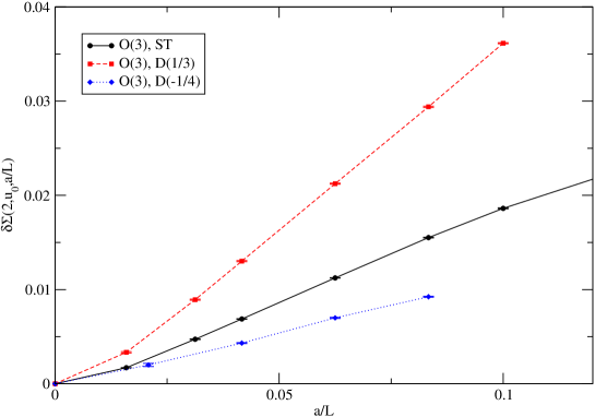
Figure 2: $\delta\Sigma(2,u_{0},a/L)$ is plotted for the O(3) ST, D(1/3) and D(-1/4) lattice actions.

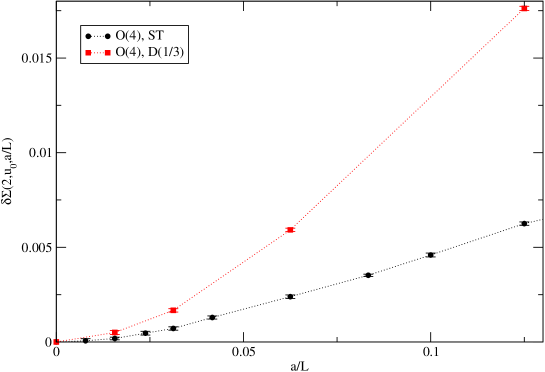
Figure 3: $\delta\Sigma(2,u_{0},a/L)$ for the O(4) ST and D(1/3) actions.

In the ratio of artifacts for different actions the unknown non-perturbative coefficient $D_{1}^{X}(\Lambda)$ in (3.125),(3.126) cancels. Expressing the ratio in terms of $\beta_{\mathrm{eff}}^{\mathrm{ST}}$ one has

$$\frac{\delta^{X}(\lambda_{0},a)}{\delta^{X}_{\mathrm{ST}}(\lambda_{0\mathrm{ST}},a)}=e_{0}\left(1+(\rho-\rho_{\mathrm{ST}})\frac{1}{\beta_{\mathrm{eff}}^{\mathrm{ST}}}+\ldots\right)\,,$$ (4.154)

where

$$\rho=\frac{1}{2\pi}\left(r^{(2)}+\frac{n}{n-2}\psi\right)\,.$$ (4.155)

The values for these constants for various actions are summarized in Table 6.

$n$	Action	$\psi/(2\pi)$	$r^{(2)}/(2\pi)$	$\rho$	$\rho-\rho_{\mathrm{ST}}$
3	ST	$0.37031535$	$-1.13861509$	$-0.02766903$
	D(1/3)	$0.58672731$	$-1.56413634$	$\phantom{-}0.19604560$	$0.22371463$
	D($-1/4$)	$0.26551678$	$-0.13328534$	$\phantom{-}0.66326502$	$0.69093405$
	SYM	$0.24344345$
4	ST	$0.49063070$	$-0.72946015$	$\phantom{-}0.25180125$
	D(1/3)	$0.79446745$	$-0.96233225$	$\phantom{-}0.62660266$	$0.37480141$
	D($-1/4$)	$0.35356625$	$\phantom{-}0.22986274$	$\phantom{-}0.93699525$	$0.68519400$
	SYM	$0.31658887$
8	ST	$0.97189212$	$-0.58931931$	$\phantom{-}0.70653685$

Table 6: Values of constants appearing in the description of the cutoff effects for different actions.

Figures 4.-8. show the values of $\delta\Sigma(2,u_{0},a/L)(L/a)^{2}$ vs. the corresponding $\beta$ values. The 2-parameter fits are the predictions from (3.125),(3.126), where the overall constant and the sub-subleading correction coefficient are fitted, while the value of $r^{(2)}$ is fixed to the known value.

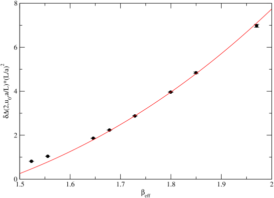
Figure 4: $\delta\Sigma(2,u_{0},a/L)(L/a)^{2}$ for O(3), ST action. The solid line is the fit $3.1320(\beta^{3}+c\beta^{2}-0.4883\beta)$, with $c=r^{(2)}/(2\pi)=-1.1386$ fixed.

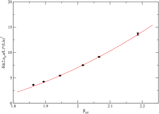
Figure 5: $\delta\Sigma(2,u_{0},a/L)(L/a)^{2}$ for O(3), D(1/3) action. The solid line is the fit $5.4803(\beta^{3}+c\beta^{2}-0.2309\beta)$, with $c=r^{(2)}/(2\pi)=-1.5641$ fixed.

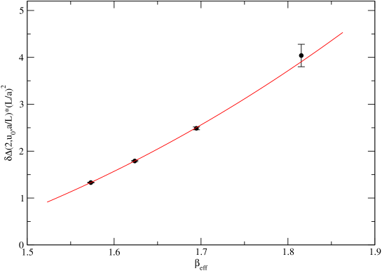
Figure 6: $\delta\Sigma(2,u_{0},a/L)(L/a)^{2}$ for O(3), D($-1/4$) action. The solid line is the fit $1.6566(\beta^{3}+c\beta^{2}-1.7554\beta)$, with $c=r^{(2)}/(2\pi)=-0.1333$ fixed.

Figure 7: $\delta\Sigma(2,u_{0},a/L)(L/a)^{2}$ for O(4), ST action. The solid line is the fit $0.185(\beta^{2}+c\beta-2.170)$, with $c=r^{(2)}/(2\pi)=-0.7295$ fixed.

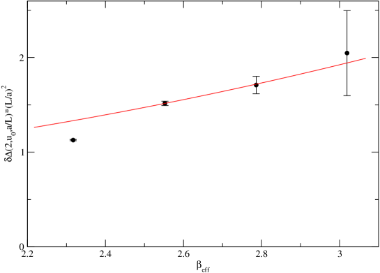
Figure 8: $\delta\Sigma(2,u_{0},a/L)(L/a)^{2}$ for O(4), D(1/3) action. The solid line is the fit $0.199(\beta^{2}+c\beta+3.566)$, with $c=r^{(2)}/(2\pi)=-0.9623$ fixed.

A further check is provided by the ratio of artifacts. For the O(3) case the ratios for D(1/3)/ST and D($-1/4$)/ST actions are shown in Fig. 9 where the data show a remarkable agreement with the parameter-free prediction in (4.154). (Note however that it is possible that this few percent agreement is due to an accidentally very small coefficient of the next, $1/\beta^{2}$, term.)

The corresponding ratio for the O(4) case is shown in Fig. 10. Although the agreement is poorer in this case, at larger $\beta$ (for $L/a=32,\,64$) the data seem to approach the prediction.

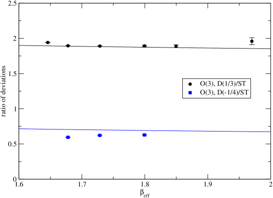
Figure 9: Ratio of deviations $\delta\Sigma(2,u_{0},a/L)$ for the D(1/3)/ST and D($-1/4$)/ST actions vs. $\beta_{\mathrm{eff}}^{\mathrm{ST}}$ for the O(3) model. The solid lines are the predictions $5/3(1+0.224/\beta_{\mathrm{eff}}^{\mathrm{ST}})$, and $1/2(1+0.691/\beta_{\mathrm{eff}}^{\mathrm{ST}})$.

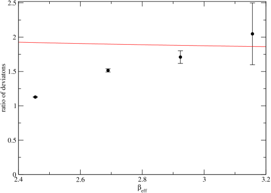
Figure 10: Ratio of deviations $\delta\Sigma(2,u_{0},a/L)$ for the D(1/3) and ST actions vs. $\beta_{\mathrm{eff}}$ for O(4). The solid line is the prediction $5/3(1+0.375/\beta_{\mathrm{eff}}^{\mathrm{ST}})$.

In [?],[?] the cut-off effects for the step scaling function were measured for O(4) and O(8) at $u_{0}=1.0595$ with the ST action. Since our errors for the O(4) case are considerably smaller, we analyse here only the O(8) data from these papers. Fig.11 shows that the MC data of [?],[?] are also consistent with the analytic predictions. (For O(8) one has $\sigma(2,u_{0})=1.345757$ at $u_{0}=1.0595$.)

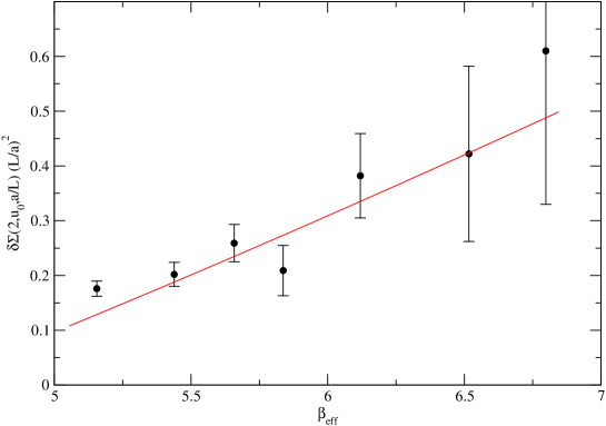
Figure 11: $\delta\Sigma(2,u_{0},a/L)(L/a)^{2}$ for O(8), ST action. The solid line is the fit $0.093(\beta^{4/3}+c\beta^{1/3}-6.50)$, with $c=r^{(2)}/(2\pi)=-0.5893$ fixed.

5 Conclusions

The main motivation of this work was to explain how the apparently linear artifacts found in ref. [?] can be reconciled with standard expectations. We have shown that the data, although astonishingly linear as function of the lattice spacing, can equally well be described by a more complicated formula we calculated using Symanzik’s theory of lattice artifacts.

Although both type of fits describe the data well, we think that by now there is no doubt that the conservative description of lattice artifacts based on Symanzik’s effective action is correct and there is no unexpected new physics behind the phenomenon (as originally suspected). Our arguments can be summarized as follows.

1) Since ref. [?] appeared, the exact continuum limit has been calculated [?] by bootstrap techniques and using this extra piece of information we see that the “linear” fits of Fig. 1 must be bent a little, as seen in Fig. 2. In other words, continuum extrapolations based on “linear” fits would miss the exact result by about 0.002.

2) Lattice artifacts normally decrease very rapidly as $a^{2}$, but here this is partially compensated by the cubic logarithmic increase of the $\beta^{3}$ factor for O$(3)$. This increase is further enhanced by the relatively large negative coefficient of the subleading term. As can be seen in Fig. 4, the logarithmic correction factor increases by about an order of magnitude between $\beta=1.6$ and $\beta=2.0$. This can mimic a $1/a$-like increase in our limited range of $\beta$.

3) The correctness of the effective action description is further corroborated by its parameter-free prediction for the ratios of artifacts, which agrees very well with the measured values (see Fig. 9 and Fig. 10 for the less spectacular O$(4)$ case).

4) In the large $n$ limit our formula reproduces the results of refs. [?,?,?].

After completing this long computation we arrived at the sobering conclusion: there are no linear artifacts and Symanzik’s theory describes the data well. But it was nevertheless useful to go through the steps of the calculation because it provided us with the opportunity to learn about Symanzik’s theory of artifacts and improvement. Similar computations should, in our opinion, accompany precision lattice studies of QCD in order to control and better estimate systematic errors arising from lattice artifacts for extrapolations to the continuum limit.

Appendix Appendix A: Anomalous dimensions of the dimension 4 operators

A.1 Scalar operators

The one-loop mixing matrix for dimension four invariant Lorentz scalars has been first computed by Brézin et al. [?] using the basis (2.28) . It is given by (2.26) with

$$2\pi w_{ij}=\begin{pmatrix}4-2n&-4&0&-\frac{n}{2}&0\\ -2&2-2n&0&-\frac{n+2}{4}&0\\ 4&-16&2-n&-2&4(n-1)\\ -4&16&0&4-n&4(1-n)\\ 1&-4&\frac{1}{4}&0&2\end{pmatrix}\,.$$ (A.156)

In Fig. 12 we show the diagrams which are needed for the renormalization of operators ${\cal O}_{1}$ and ${\cal O}_{2}$ to 1-loop order.

Figure 12: 1-loop contributions to the renormalization of operators ${\cal O}_{1}$ and ${\cal O}_{2}$. Full circles represent the (4 or 6-leg part) of the operators, full squares stand for the 4-point interaction vertex of the model.

We will now simplify the mixing problem using some operator identities. The identities can be derived by making in (2.3) the infinitesimal change of variables

$$\delta\pi^{i}=\delta\omega Q^{i}\,,$$ (A.157)

where $\delta\omega$ is an infinitesimal parameter and $Q^{i}$ is an arbitrary local expression of the fields and sources. The corresponding change in the action is

$$\delta{\cal A}=-\delta\omega\int{\rm d}^{D}x\left(\square\pi^{i}-\alpha\pi^{i}+\frac{1}{g_{0}}I^{i}\right)Q^{i}$$ (A.158)

and since the measure $\left({\cal D}\pi\right)$ is invariant in dimensional regularization under any local change of variables we have

$${\cal Z}[I]=\int\left({\cal D}\pi\right)\,{\rm e}^{-{\cal A}-\delta{\cal A}}={\cal Z}[I]-\int\left({\cal D}\pi\right)\,\delta{\cal A}{\rm e}^{-{\cal A}}\,,$$ (A.159)

leading to the operator identity $\delta{\cal A}=0$. Thus we have

$$\left(\square\pi^{i}-\alpha\pi^{i}+\frac{1}{g_{0}}I^{i}\right)Q^{i}\approx 0\,,$$ (A.160)

where $\approx$ means operator identity for the corresponding space integrals.

We now consider the infinitesimal transformations corresponding to respectively

$$Q^{i}=\left\{g_{0}^{2}\left(\partial_{\mu}S\cdot\partial_{\mu}S\right)\pi^{i}\,,g_{0}^{2}\left(I\cdot S+\bar{\alpha}\right)\pi^{i},g_{0}I^{i}+g_{0}^{2}\bar{\alpha}\pi^{i},g_{0}^{2}\square\pi^{i}\right\}$$ (A.161)

and find the identities

$$\begin{split}\left(I\cdot S\right)\left(\partial_{\mu}S\cdot\partial_{\mu}S\right)&\approx\bar{\alpha}\,\partial_{\mu}S\cdot\partial_{\mu}S\,,\\ \left(I\cdot S\right)^{2}&\approx\bar{\alpha}^{2}\,,\\ I^{2}+I\cdot\square S+\left(I\cdot S\right)\,(\partial_{\mu}S\cdot\partial_{\mu}S)&\approx\bar{\alpha}^{2}\,,\\ I\cdot\square S-(\partial_{\mu}S\cdot\partial_{\mu}S)^{2}+\square S\cdot\square S&\approx-\bar{\alpha}(\partial_{\mu}S\cdot\partial_{\mu}S)\,,\end{split}$$ (A.162)

respectively. Here we have introduced the operator

$$\bar{\alpha}=\alpha+\partial_{\mu}S\cdot\partial_{\mu}S\,.$$ (A.163)

We see that insertions of the apparently O$(n)$ non-invariant operators ${\cal O}_{4}$ and ${\cal O}_{5}$ are equivalent to inserting the manifestly invariant ones in (A.162). There are no further identities independent of the ones in (A.162). This can be shown by using the continuum analog of the lattice considerations of ref. [?].

It will be convenient to use a new basis of operators. We keep the “hard” operators ${\cal O}_{1}$ and ${\cal O}_{2}$ but instead of the rest we first introduce $W,U$ and $V$, where

$$\begin{split}4W&=\bar{\alpha}\,\partial_{\mu}S\cdot\partial_{\mu}S\,,\\ 8U&=\bar{\alpha}^{2}\,,\\ 2V&=\square S\cdot\square S-(\partial_{\mu}S\cdot\partial_{\mu}S)^{2}+\bar{\alpha}^{2}\,.\end{split}$$ (A.164)

This basis change corresponds to

$$\begin{split}{\cal O}_{3}&=V-4U+4{\cal O}_{1}\,,\\ {\cal O}_{4}&=2W-4{\cal O}_{1}\,,\\ {\cal O}_{5}&=U-W+{\cal O}_{1}\,.\end{split}$$ (A.165)

Further we introduce the combinations

$$\overline{U}_{3}=W-2U+\frac{1}{2}V\,,\qquad\qquad\overline{U}_{4}=U-\frac{1}{4n}V\,,\qquad\qquad\overline{U}_{5}=V\,.$$ (A.166)

Now the operator identities can be rewritten as

$$\begin{split}\overline{U}_{3}&\approx-\frac{1}{4}I\cdot\square S\,,\\ \overline{U}_{4}&\approx\frac{1}{8}I^{a}I^{b}\tau^{ab}\,,\\ \overline{U}_{5}&\approx\frac{1}{2}I^{2}\,,\end{split}$$ (A.167)

where

$$\tau^{ab}=S^{a}S^{b}-\frac{1}{n}\delta^{ab}\,.$$ (A.168)

Inserting the above identities into the generating functional (2.19) we can derive useful identities for the correlation functions of the operators $\overline{U}_{j}\,,j=3,4,5$. These are best formulated in Fourier space. We define, as usual,

$$\begin{split}\int{\rm d}^{D}x\,{\rm e}^{i(p_{1}x_{1}+\dots+p_{r}x_{r})}\,&{\cal G}^{a_{1}\dots a_{r}}_{[\bar{U}]}(x_{1},\dots,x_{r})\\ &=(2\pi)^{D}\delta(p_{1}+\dots+p_{r})\,\widetilde{\cal G}^{a_{1}\dots a_{r}}_{[\bar{U}]}(p_{1},\dots,p_{r})\end{split}$$ (A.169)

for correlation functions with and without operator insertions. With this notation we have

$$\widetilde{\cal G}_{\overline{U}_{3}}^{a_{1}\dots a_{r}}(p_{1},\dots,p_{r})=\frac{g_{0}^{2}}{4}\,\left(\sum_{k=1}^{r}p_{k}^{2}\right)\,\widetilde{\cal G}^{a_{1}\dots a_{r}}(p_{1},\dots,p_{r})\,.$$ (A.170)

From this formula it is clear that the operator $\overline{U}_{3}$ is renormalized multiplicatively with renormalization constant

$$Z_{\overline{U}_{3}}=\frac{1}{Z_{1}}=1-\frac{(2-n)g^{2}}{2\pi\varepsilon}+\dots$$ (A.171)

For $\overline{U}_{4}$ we have

$$\begin{split}\widetilde{\cal G}_{\overline{U}_{4}}^{a_{1}\dots a_{r}}(p_{1},\dots,p_{r})&=\frac{g_{0}^{4}}{4}\,\widetilde{\cal G}_{\tau}^{a_{1}a_{2};a_{3}\dots a_{r}}(p_{1}+p_{2};p_{3},\dots,p_{r})+\left[\begin{pmatrix}r\\ 2\end{pmatrix}-1\right]{\rm perms}\\ &+\frac{m^{2}g_{0}^{2}}{4}\,\widetilde{\cal G}_{\tau}^{a_{1}n;a_{2}\dots a_{r}}(p_{1};p_{2},\dots,p_{r})+\left[r-1\right]{\rm perms}\\ &+\frac{m^{4}}{8}\,\widetilde{\cal G}_{\tau}^{nn;a_{1}\dots a_{r}}(0;p_{1},\dots,p_{r})\,,\end{split}$$ (A.172)

where

$$\widetilde{\cal G}_{\tau}^{ab;a_{1}\dots a_{r}}(p;p_{1},\dots,p_{r})$$ (A.173)

is the Fourier space correlation function of the local operator $\tau^{ab}$ at momentum $p$. Actually, (A.172) is valid for $r>2$ only. For $r=2$ we have

$$\begin{split}\widetilde{\cal G}_{\overline{U}_{4}}^{a_{1}a_{2}}(p,-p)&=\frac{g_{0}^{4}}{4}\langle\tau^{a_{1}a_{2}}\rangle+\frac{m^{2}g_{0}^{2}}{4}\widetilde{\cal G}_{\tau}^{a_{1}n;a_{2}}(p;-p)\\ &+\frac{m^{2}g_{0}^{2}}{4}\widetilde{\cal G}_{\tau}^{a_{2}n;a_{1}}(-p;p)+\frac{m^{4}}{8}\widetilde{\cal G}_{\tau}^{nn;a_{1}a_{2}}(0;p,-p)\,.\end{split}$$ (A.174)

Since in (A.172) (and in (A.174)) all terms require the same overall renormalization constant, the operator $\overline{U}_{4}$ renormalizes multiplicatively with renormalization constant

$$Z_{\overline{U}_{4}}=\frac{ZZ_{\tau}}{Z_{1}^{2}}=1-\frac{(3-2n)g^{2}}{2\pi\varepsilon}+\dots,$$ (A.175)

where we have used the result

$$Z_{\tau}=1+\frac{ng^{2}}{2\pi\varepsilon}+\dots$$ (A.176)

Finally for $\overline{U}_{5}$ we find

$$\begin{split}\widetilde{\cal G}_{\overline{U}_{5}}^{a_{1}\dots a_{r}}(p_{1},\dots,p_{r})&=(2\pi)^{D}\delta(p_{1}+p_{2})g_{0}^{4}\,\widetilde{\cal G}^{a_{3}\dots a_{r}}(p_{3},\dots,p_{r})\delta^{a_{1}a_{2}}+\left[\begin{pmatrix}r\\ 2\end{pmatrix}-1\right]{\rm perms}\\ &+(2\pi)^{D}\delta(p_{1})\delta^{a_{1}n}m^{2}g_{0}^{2}\,\widetilde{\cal G}^{a_{2}\dots a_{r}}(p_{2},\dots,p_{r})+\left[r-1\right]{\rm perms}\end{split}$$ (A.177)

for $r>2$ and

$$\widetilde{\cal G}_{\overline{U}_{5}}^{a_{1}a_{2}}(p,-p)=g_{0}^{4}\delta^{a_{1}a_{2}}+2m^{2}g_{0}^{2}\delta^{a_{1}n}\delta^{a_{2}n}\langle\sigma\rangle\delta(p)(2\pi)^{D}$$ (A.178)

for $r=2$. Again, $\overline{U}_{5}$ renormalizes multiplicatively with

$$Z_{\overline{U}_{5}}=\frac{Z}{Z_{1}^{2}}=1-\frac{(3-n)g^{2}}{2\pi\varepsilon}+\dots$$ (A.179)

We can check the results (A.171), (A.175) and (A.179) by using the mixing matrix (A.156). We define the linear operator

$$C({\cal O}_{i})=2\pi w_{ij}{\cal O}_{j}$$ (A.180)

and then find

$$C(\overline{U}_{3})=(2-n)\overline{U}_{3}\,,\qquad C(\overline{U}_{4})=(3-2n)\overline{U}_{4}\quad{\rm and}\quad C(\overline{U}_{5})=(3-n)\overline{U}_{5}\,.$$ (A.181)

There are two other linear combinations $\overline{U}_{i}\,,i=1,2$ diagonalizing the one-loop mixing matrix (A.156) with

$$C(\overline{U}_{1})=2\overline{U}_{1}\qquad\qquad{\rm and}\qquad\qquad C(\overline{U}_{2})=(4-2n)\overline{U}_{2}\,.$$ (A.182)

The relations between the bases are given by

$$\overline{U}_{i}={\cal S}_{ij}{\cal O}_{j}\,,$$ (A.183)

with the matrix ${\cal S}$ given by

$${\cal S}=\begin{pmatrix}\frac{n+4}{2n-1}&-2&\frac{(n-2)(n+1)}{2n(2n-1)}&\frac{(n-2)(n+1)}{2n(2n-1)}&\frac{2(n-2)(n+1)}{2n-1}\\ 5&-2&-\frac{1}{n-2}&\frac{2n-5}{n-2}&4\\ 0&0&\frac{1}{2}&\frac{1}{2}&0\\ 1&0&-\frac{1}{4n}&\frac{n-1}{2n}&\frac{n-1}{n}\\ 0&0&1&2&4\end{pmatrix}\,.$$ (A.184)

For later use we also write down the inverse of this matrix

$${\cal S}^{-1}=\begin{pmatrix}\frac{1}{n-1}&-\frac{1}{n-1}&\frac{n^{2}-2n-4}{n(n-2)}&\frac{2(n+4)}{2n-1}&-\frac{(n^{2}-n-4)}{2n(n-1)}\\ \frac{1}{2(n-1)}&-\frac{n}{2(n-1)}&\frac{n^{2}-4n-4}{2n(n-2)}&\frac{5n+2}{2n-1}&-\frac{(n^{2}-3n-2)}{4n(n-1)}\\ \frac{4}{n-1}&-\frac{4}{n-1}&\frac{4(n^{2}-2n-4)}{n(n-2)}&\frac{36}{2n-1}&-\frac{(n^{2}-9)}{n(n-1)}\\ -\frac{4}{n-1}&\frac{4}{n-1}&-\frac{2(n^{2}-2n-8)}{n(n-2)}&-\frac{36}{2n-1}&\frac{n^{2}-9}{n(n-1)}\\ \frac{1}{n-1}&-\frac{1}{n-1}&-\frac{4}{n(n-2)}&\frac{9}{2n-1}&-\frac{(n-9)}{4n(n-1)}\end{pmatrix}\,.$$ (A.185)

A.2 Tensor operators

Here we discuss some properties of the four-index symmetric tensor operators defined in (2.30) and (2.31).

Let $X_{\mu\nu\rho\sigma}$ be a tensor operator, totally symmetric in its indices $\mu$, $\nu$, $\rho$, $\sigma$. We can construct the corresponding totally symmetric, traceless tensor operator $\widehat{X}_{\mu\nu\rho\sigma}$ by subtracting trace terms as follows.

$$\begin{split}\widehat{X}_{\mu\nu\rho\sigma}&=X_{\mu\nu\rho\sigma}-\frac{1}{D+4}\Big{\{}g_{\mu\nu}\xi_{\rho\sigma}+g_{\rho\sigma}\xi_{\mu\nu}+g_{\mu\rho}\xi_{\nu\sigma}+g_{\nu\sigma}\xi_{\mu\rho}\\ &+g_{\mu\sigma}\xi_{\nu\rho}+g_{\nu\rho}\xi_{\mu\sigma}\Big{\}}+\frac{\bar{\xi}}{(D+2)(D+4)}\Big{\{}g_{\mu\nu}g_{\rho\sigma}+g_{\mu\rho}g_{\nu\sigma}+g_{\mu\sigma}g_{\nu\rho}\Big{\}}\,,\end{split}$$ (A.186)

where

$$\xi_{\rho\sigma}=X_{\alpha\alpha\rho\sigma},\qquad\qquad{\rm and}\qquad\qquad\bar{\xi}=X_{\alpha\alpha\beta\beta}\,.$$ (A.187)

In the effective Lagrangian there are operators of the form $\sum_{\mu=1}^{D}X_{\mu\mu\mu\mu}$, which can be rewritten, using (A.186) as

$$\sum_{\mu=1}^{D}X_{\mu\mu\mu\mu}=\sum_{\mu=1}^{D}\widehat{X}_{\mu\mu\mu\mu}+\frac{3}{4-\varepsilon}X_{\alpha\alpha\beta\beta}\,.$$ (A.188)

If we apply this procedure to the operator $t_{\mu\nu\rho\sigma}$ in (2.30)we get

$$\sum_{\mu=1}^{D}S\cdot\partial^{4}_{\mu}\,S=A+\frac{6}{4-\varepsilon}{\cal O}_{3}\,,$$ (A.189)

where $A$ is defined in (2.32). The traceless symmetric tensor operator $\widehat{t}_{\mu\nu\rho\sigma}$ can mix under renormalization with other traceless symmetric tensor operators only (which must have the same values for other quantum numbers). All tensor components renormalize the same way and using this property we can simplify the renormalization problem by considering the $\widehat{t}_{++++}$ tensor component, where

$$V_{+}=V_{1}+iV_{2}$$ (A.190)

for any vector. Great simplification occurs in PT calculations for this tensor component since $g_{++}=0$ and many diagrams vanish, and it is thus easier to renormalize

$$\bar{A}=\widehat{t}_{++++}=\partial^{2}_{+}S\cdot\partial^{2}_{+}S$$ (A.191)

instead of $A$ itself. (Note that we are considering operators at zero momentum, i.e. their space integrals.)

$\widehat{t}_{\mu\nu\rho\sigma}$ can mix under renormalization with $\widehat{k}_{\mu\nu\rho\sigma}$ given in (2.31). For this operator we find

$$\sum_{\mu=1}^{D}\left(\partial_{\mu}S\cdot\partial_{\mu}S\right)^{2}=B+\frac{8}{4-\varepsilon}\left({\cal O}_{1}+2{\cal O}_{2}\right)\,,$$ (A.192)

where $B$ is defined in (2.33). For convenience we define

$$\bar{B}=\widehat{k}_{++++}=\left(\partial_{+}S\cdot\partial_{+}S\right)^{2}\,.$$ (A.193)

There are no other spin–four, dimension–four O$(n)$ invariant operators, therefore we have a $2\times 2$ renormalization problem here. By calculating the matrix elements of $\bar{A}$, $\bar{B}$ we find that the mixing matrix is diagonal,

$$K_{ij}=\delta_{ij}+\frac{g^{2}(n-2)}{2\pi\varepsilon}\begin{pmatrix}0&0\\ 0&1\end{pmatrix}+\dots,$$ (A.194)

for the operators

$$U_{6}=\frac{1}{g_{0}^{2}}A\,,\qquad\qquad U_{7}=\frac{1}{g_{0}^{2}}B\,.$$ (A.195)

A.3 2-loop Mixing matrix elements

For the computation of the mixing coefficients $\nu^{(2)}_{ij}$, we worked in the Brézin et al basis (2.28) and computed the corresponding $p_{ij}$ coefficients of the $g^{4}/\varepsilon$ terms in (2.26). From the relation between the bases (A.184) the $\nu_{ij}^{(2)}$ are then given by

$$\nu_{ij}^{(2)}=-\frac{(n-2)}{(2\pi)^{2}}\delta_{ij}+{\cal S}_{ik}p_{kl}({\cal S}^{-1})_{lj}\,.$$ (A.196)

For the computation of $r^{(2)}_{\rm III}$ we only require $\nu_{ij}^{(2)}$ for $i,j=1,2$. For this purpose we only need the $p_{ij}$ for $i=1,2$ because using the fact that $K_{ij}=0$ for $i=3,4,5$ and $j=1,2$ we have

$$\sum_{k=1}^{5}{\cal S}_{ik}(p{\cal S}^{-1})_{kj}=\sum_{k=1}^{2}{\cal T}_{ik}(p{\cal S}^{-1})_{kj}\,,\,\,\,\,i,j\in\{1,2\}\,,$$ (A.197)

with

$${\cal T}_{ik}={\cal S}_{ik}-\sum_{r,s=3}^{5}{\cal S}_{ir}\sigma_{rs}{\cal S}_{sk}\,,\,\,\,\,i,k\in\{1,2\}\,,$$ (A.198)

where $\sigma$ is the inverse of the lower $3\times 3$ diagonal block of ${\cal S}$ (i.e. $\sum_{s=3}^{5}\sigma_{rs}{\cal S}_{st}=\delta_{rt}$). For the computation of $p_{ij}$ for $j=3,4,5$ we need to compute the divergent parts of insertions of ${\cal O}_{i}$ in the 2-point pion correlation functions (with just up to one interaction vertex), and for the computation of $p_{ij}$ for $1,2$ we need the analogous computation for the insertions of ${\cal O}_{i}$ in the 4-point pion correlation functions (with up to two interaction vertices).

The computation is again too lengthy to present the details here; we just list the relevant Feynman diagrams in Fig. 13. Note that the 1-loop contribution corresponding to the diagram $b$ in Fig. 12 is only a wave function renormalization. Analogous contributions (with wave function renormalization on one or two external legs) are not shown among the diagrams of Fig. 13. Diagram $d$ in Fig. 12 contains an internal contraction line and thus vanishes in the limit $m\to 0$. Diagrams containing similar internal contractions are not shown in Fig. 13 either.

Figure 13: 2-loop contributions to the renormalization of operators ${\cal O}_{1}$ and ${\cal O}_{2}$. Full circles represent the (4, 6 or 8-leg part) of the operators, full squares stand for the (4-point or 6-point) interaction vertex of the model.

We checked that the $1/\varepsilon^{2}$ divergences were as expected from the RG considerations, and from the $1/\varepsilon$ divergences we finally obtained

$$\begin{split}(2\pi)^{2}p_{1j}&=\left\{\frac{7n}{2}-11\,,-9n+19\,,\frac{n}{4}\,,\frac{n-3}{2}\,,-n+1\right\}\,,\\ (2\pi)^{2}p_{2j}&=\left\{-\frac{13n}{4}+7\,,\frac{3n-13}{2}\,,\frac{n+2}{8}\,,-\frac{n-1}{2}\,,-\frac{n(n-1)}{2}\right\}\,.\end{split}$$ (A.199)

This yields

$$\begin{split}(2\pi)^{2}\nu_{11}^{(2)}&=-\frac{3(2n^{2}-5n+5)}{2(n-1)}\,,\\ (2\pi)^{2}\nu_{21}^{(2)}&=\frac{n(n-4)}{(n-1)}\,.\end{split}$$ (A.200)

Appendix Appendix B: Lattice perturbation theory

B.1 Perturbation theory with periodic bc

We consider a volume $V=N^{2}$ with periodic boundary conditions in each direction

$$S(x+N\hat{\mu})=S(x)\,,\,\,\mu=1,2\,.$$ (B.201)

Let ${\cal O}$ be an O$(n)$ invariant observable. For $\lambda_{0}\to 0$ zero modes appear due to the O$(n)$ invariance. To avoid this Hasenfratz [?] used the Fadeev-Popov trick:

$$\langle{\cal O}\rangle=\frac{1}{Z}\int{\rm d}^{n}r\,\int[{\rm d}S]{\rm e}^{-{\cal A}}\delta\left(r-\sum_{x}S(x)\right){\cal O}[S]\,.$$ (B.202)

Because of the O$(n)$ invariance the inner integral is independent of the direction of $r$. Take $r=|r|n_{0}\,,\,\,n_{0}=(0,0,\dots,0,1)$ and set

$$S(x) =\left(\lambda_{0}\pi(x),\sigma(x)\right)$$ (B.203)

$$\sigma(x) =\sqrt{1-\lambda_{0}^{2}\pi(x)^{2}}$$ (B.204)

where $\pi(x)$ has $n-1$ components $\pi^{j}(x)\,,j=1,\dots,n-1$ . Then

$$\begin{split}\langle{\cal O}\rangle&=\frac{1}{Z}\int\left[\prod_{x}{\rm d}^{n-1}\pi(x)\,\frac{1}{\sigma(x)}\right]\left(\frac{1}{V}\sum_{x}\sigma(x)\right)^{n-1}\delta\left(\sum_{x}\pi(x)\right){\cal O}\,{\rm e}^{-{\cal A}}\\ &\\ &=\frac{1}{Z_{\rm eff}}\int\left[\prod_{x}{\rm d}^{n-1}\pi(x)\right]\delta\left(\sum_{x}\pi(x)\right){\cal O}\,{\rm e}^{-{\cal A}_{\rm eff}}\,,\end{split}$$ (B.205)

with

$${\cal A}_{\rm eff}={\cal A}+\sum_{x}\ln\sigma(x)-(n-1)\ln\left(\frac{1}{V}\sum_{x}\sigma(x)\right)\,.$$ (B.206)

Then when one expands for $\lambda_{0}\to 0$ no zero modes occur because of the delta function.

In the following we restrict results to the infinite volume limit.

B.2 1-loop connected 4-point function

The leading orders of the connected 4-point function have been given in subsect. 2.2.2. Here we give the result for $\widetilde{C}_{2}$ and consider the coefficients of powers of $(n-1)$ separately:

$$\widetilde{C}_{2}=\sum_{r=0}^{2}(n-1)^{r}\widetilde{C}_{2}^{[r]}\,.$$ (B.207)

First for $\widetilde{C}_{2}^{[2]}$ we obtain simply:

$$\widetilde{C}_{2}^{[2]}(p_{1},q_{1};p_{2},q_{2})=\frac{1}{2}\frac{1}{K_{p_{1}}K_{q_{1}}K_{p_{2}}K_{q_{2}}}K_{p_{1}+q_{1}}F(p_{1}+q_{1})\,.$$ (B.208)

Next for $\widetilde{C}_{2}^{[1]}$ we get:

$$\begin{split}&\widetilde{C}_{2}^{[1]}(p_{1},q_{1};p_{2},q_{2})=\frac{1}{2}\frac{1}{K_{p_{1}}K_{q_{1}}K_{p_{2}}K_{q_{2}}}\left[K_{p_{1}+p_{2}}F(p_{1}+p_{2})+K_{p_{1}+q_{2}}F(p_{1}+q_{2})\right]\\ &-\frac{1}{2}\left[F(p_{1})+F(q_{1})\right]\widetilde{C}_{1}^{(1)}(p_{1},q_{1};p_{2},q_{2})-\frac{1}{2}\left[F(p_{2})+F(q_{2})\right]\widetilde{C}_{1}^{(2)}(p_{1},q_{1};p_{2},q_{2})\\ &+\frac{1}{2}\frac{1}{K_{p_{2}}K_{q_{2}}}\left[\frac{F(p_{1})}{K_{p_{1}}}+\frac{F(q_{1})}{K_{q_{1}}}\right]+\frac{1}{2}\frac{1}{K_{p_{1}}K_{q_{1}}}\left[\frac{F(p_{2})}{K_{p_{2}}}+\frac{F(q_{2})}{K_{q_{2}}}\right]\\ &+\frac{1}{K_{p_{1}}K_{q_{1}}K_{p_{2}}K_{q_{2}}}\left[k_{p_{1}}+k_{q_{1}}+k_{p_{2}}+k_{q_{2}}\right]\\ &-\frac{1}{K_{p_{1}}K_{q_{1}}K_{p_{2}}K_{q_{2}}}K_{p_{1}+q_{1}}\left[\frac{k_{p_{1}}}{K_{p_{1}}}+\frac{k_{q_{1}}}{K_{q_{1}}}+\frac{k_{p_{2}}}{K_{p_{2}}}+\frac{k_{q_{2}}}{K_{q_{2}}}\right]\\ &+\frac{K_{p_{1}+q_{1}}}{K_{p_{1}}K_{q_{1}}K_{p_{2}}K_{q_{2}}}\left[\overline{J}_{1}(p_{1},q_{1})+\overline{J}_{1}(p_{2},q_{2})\right]\\ &+\frac{1}{K_{p_{1}}K_{q_{1}}K_{p_{2}}K_{q_{2}}}\left[\overline{Z}_{4}(p_{1},p_{2},q_{1})+\overline{Z}_{4}(p_{1},q_{2},q_{1})\right]\\ &-K_{p_{1}+q_{1}}\left[\frac{\overline{T}_{1}(p_{1},q_{1})}{K_{p_{2}}K_{q_{2}}}+\frac{\overline{T}_{1}(p_{2},q_{2})}{K_{p_{1}}K_{q_{1}}}\right]\,,\end{split}$$ (B.209)

where

$$\overline{Z}_{2}(p,q) =\int_{k}\left[\frac{K_{k-p-q}}{K_{k}K_{k-p}}-\frac{K_{p+q}}{K_{k}K_{p}}-\frac{K_{q}}{K_{p}K_{k-p}}\right]\,,$$ (B.210)

$$\overline{J}_{1}(p,q) =\overline{Z}_{2}(-p-q,p)=\overline{Z}_{2}(-p-q,q)$$

$$=\int_{k}\left[\frac{K_{k}}{K_{k-p}K_{k+q}}-\frac{K_{p}}{K_{p+q}K_{k-p}}-\frac{K_{q}}{K_{p+q}K_{k+q}}\right]\,,$$ (B.211)

$$\overline{Z}_{4}(p,q,r) =\int_{k}\left[\frac{K_{k-p}K_{k+r}}{K_{k}K_{k-p-q}}-1-\frac{K_{p}K_{r}}{K_{k}K_{p+q}}-\frac{K_{p+q+r}K_{q}}{K_{p+q}K_{k-p-q}}\right]\,,$$ (B.212)

$$\overline{T}_{1}(p,q) =\int_{k}\left[\frac{1}{K_{k}K_{k-p}K_{k+q}}-\frac{1}{K_{k}K_{p}K_{q}}-\frac{1}{K_{p}K_{k-p}K_{p+q}}-\frac{1}{K_{q}K_{p+q}K_{k+q}}\right]\,.$$ (B.213)

Finally for $\widetilde{C}_{2}^{[0]}$ we get:

$$\begin{split}&\widetilde{C}_{2}^{[0]}(p_{1},q_{1};p_{2},q_{2})=\frac{1}{K_{p_{2}}K_{q_{2}}}\left[\frac{F(p_{1})}{K_{p_{1}}}+\frac{F(q_{1})}{K_{q_{1}}}\right]+\frac{1}{K_{p_{1}}K_{q_{1}}}\left[\frac{F(p_{2})}{K_{p_{2}}}+\frac{F(q_{2})}{K_{q_{2}}}\right]\\ &+\left[\frac{1}{K_{p_{2}}K_{q_{2}}}+\frac{1}{K_{p_{1}}K_{q_{1}}}\right]\left[\frac{k_{p_{1}+p_{2}}}{K_{p_{1}+p_{2}}^{2}}+\frac{k_{p_{1}+q_{2}}}{K_{p_{1}+q_{2}}^{2}}\right]\\ &+\left[\frac{1}{K_{p_{1}+p_{2}}}+\frac{1}{K_{p_{1}+q_{2}}}\right]\left[\frac{1}{K_{p_{2}}K_{q_{2}}}\left\{\frac{k_{q_{2}}}{K_{q_{2}}}+\frac{k_{p_{2}}}{K_{p_{2}}}\right\}+\frac{1}{K_{p_{1}}K_{q_{1}}}\left\{\frac{k_{q_{1}}}{K_{q_{1}}}+\frac{k_{p_{1}}}{K_{p_{1}}}\right\}\right]\\ &+\frac{2}{K_{p_{1}}K_{q_{1}}K_{p_{2}}K_{q_{2}}}\left[k_{p_{1}}+k_{q_{1}}+k_{p_{2}}+k_{q_{2}}\right]\\ &-\frac{1}{K_{p_{1}}K_{q_{1}}K_{p_{2}}K_{q_{2}}}\left[K_{p_{1}+p_{2}}+K_{p_{1}+q_{2}}\right]\left[\frac{k_{p_{1}}}{K_{p_{1}}}+\frac{k_{q_{1}}}{K_{q_{1}}}+\frac{k_{p_{2}}}{K_{p_{2}}}+\frac{k_{q_{2}}}{K_{q_{2}}}\right]\\ &-\frac{1}{K_{p_{2}}K_{q_{2}}}\left[\frac{1}{K_{p_{1}+p_{2}}}\left\{\overline{Z}_{2}(p_{1},p_{2})+\overline{Z}_{2}(q_{1},q_{2})\right\}+\frac{1}{K_{p_{1}+q_{2}}}\left\{\overline{Z}_{2}(p_{1},q_{2})+\overline{Z}_{2}(q_{1},p_{2})\right\}\right]\\ &-\frac{1}{K_{p_{1}}K_{q_{1}}}\left[\frac{1}{K_{p_{1}+p_{2}}}\left\{\overline{Z}_{2}(p_{2},p_{1})+\overline{Z}_{2}(q_{2},q_{1})\right\}+\frac{1}{K_{p_{1}+q_{2}}}\left\{\overline{Z}_{2}(p_{2},q_{1})+\overline{Z}_{2}(q_{2},p_{1})\right\}\right]\\ &+\frac{1}{K_{p_{1}}K_{q_{1}}K_{p_{2}}K_{q_{2}}}\Bigl{[}K_{p_{1}+p_{2}}\left\{\overline{J}_{1}(p_{1},p_{2})+\overline{J}_{1}(q_{1},q_{2})\right\}\\ &+K_{p_{1}+q_{2}}\left\{\overline{J}_{1}(p_{1},q_{2})+\overline{J}_{1}(q_{1},p_{2})\right\}\Bigr{]}\\ &+\frac{1}{K_{p_{1}}K_{q_{1}}K_{p_{2}}K_{q_{2}}}\Bigl{[}\overline{Z}_{4}(p_{1},q_{1},p_{2})+\overline{Z}_{4}(p_{1},q_{1},q_{2})+\overline{Z}_{4}(p_{1},p_{2},q_{2})+\overline{Z}_{4}(p_{1},q_{2},p_{2})\Bigr{]}\\ &-\frac{1}{K_{p_{2}}K_{q_{2}}}\left[\overline{T}_{2}(p_{1},q_{1},p_{2})+\overline{T}_{2}(p_{1},q_{1},q_{2})\right]-\frac{1}{K_{p_{1}}K_{q_{1}}}\left[\overline{T}_{2}(p_{2},q_{2},p_{1})+\overline{T}_{2}(p_{2},q_{2},q_{1})\right]\\ &+\overline{B}(p_{1},q_{1},p_{2})+\overline{B}(p_{1},q_{1},q_{2})+\overline{B}(p_{1},q_{2},p_{2})\,,\end{split}$$ (B.214)

where

$$\overline{T}_{2}(p,q,r)=\int_{k}\Bigl{[}\frac{K_{k-p-r}}{K_{k}K_{k-p}K_{k+q}}-\frac{K_{p+r}}{K_{k}K_{p}K_{q}}\\ -\frac{K_{r}}{K_{p}K_{k-p}K_{p+q}}-\frac{K_{p+q+r}}{K_{q}K_{p+q}K_{k+q}}\Bigr{]}\,,$$ (B.215)

$$\overline{B}(p,q,r)=\int_{k}\Bigl{[}\frac{1}{K_{k}K_{k-p}K_{k+q}K_{k-p-r}}-\frac{1}{K_{k}K_{p}K_{q}K_{p+r}}\\ -\frac{1}{K_{p}K_{k-p}K_{p+q}K_{r}}-\frac{1}{K_{q}K_{p+q}K_{k+q}K_{p+q+r}}-\frac{1}{K_{p+r}K_{r}K_{p+q+r}K_{k-p-r}}\Bigr{]}.$$ (B.216)

B.3 Lattice integrals

const.$C$	ST	D(1/3)	D($-1/4$)	SYM
$A_{0}$	$\frac{1}{4}$	$\phantom{-}0.37898718$	$\phantom{-}0.17746732$	$\phantom{-}0.17029804$
$A_{1}$	$-\frac{1}{48}$	$\phantom{-}0.03291132$	$-0.05105528$	$\phantom{-}0.01237582$
$A_{2}$	$0$	$-0.06449359$	$\phantom{-}0.03626634$	$0$
$c_{1}$	$-5\ln 2$	$-4.56434819$	$-3.06027079$	$-2.87298102$
$c_{2}$	$\frac{5}{16}\ln 2+\frac{1}{8}$	$\phantom{-}0.35045294$	$\phantom{-}0.48105013$	$\phantom{-}0.03014466$
$F_{10}$	$-\frac{5}{4\pi}\ln 2$	$-0.55231383$	$-0.16155304$	$-0.15765008$
$F_{15}^{(A)}$	$\frac{1}{2\pi}\left[-5\ln 2+\pi-1\right]$	$\phantom{-}0.09572176$	$-0.39020365$	$-0.29701963$
$F_{15}^{(B)}$	$0$	$-0.07444697$	$\phantom{-}0.03297538$	$0$
$F_{17}^{(A)}$	$\frac{1}{2\pi}\left[\pi-2\right]$	$-0.15764297$	$\phantom{-}0.31124154$	$\phantom{-}0.13997926$
$F_{17}^{(B)}$	$\frac{1}{2\pi}$	$\phantom{-}0.47746483$	$-0.07957747$	$\phantom{-}0.06287345$
$F_{17}^{(C)}$	$0$	$\phantom{-}0.09153552$	$\phantom{-}0.02817918$	$0$
$F_{28}^{(A)}$	$-0.07421002$	$\phantom{-}0.02872250$	$-0.18868881$	$-0.07852019$
$F_{28}^{(B)}$	$-0.05734358$	$-0.10135050$	$-0.00290322$	$-0.03887267$
$F_{29}$	$-0.07889581$	$-0.11486836$	$-0.05199331$	$-0.06922970$
$F_{30}^{(A)}$	$-0.05431565$	$\phantom{-}0.00882813$	$-0.13895289$	$-0.07852019$
$F_{30}^{(B)}$	$-0.07821415$	$-0.07058178$	$-0.13051244$	$-0.04738831$
$F_{30}^{(C)}$	$0$	$-0.01798155$	$\phantom{-}0.05047165$	$0$

Table 7: Constants for various actions.

The expansion in the cutoff of the functions $F(p),k_{p}$ and others appearing in $\widetilde{C}_{2}$ (which will be considered in the next subsection) involve various lattice integrals that we will first define here. They depend on the specific lattice action and hence on the associated function $K_{p}$ (2.37). We first define

$$A_{0}\delta_{\mu\nu}=-\frac{1}{2}\int_{s}\frac{1}{K_{s}}\left[K_{\mu\nu}(s)-K_{\mu\nu}(0)\right]\,,$$ (B.217)

$$A_{1}\delta_{\mu\nu\lambda\rho}+\frac{1}{3}A_{2}s_{\mu\nu\lambda\rho}=-\frac{a^{-2}}{24}\int_{s}\frac{1}{K_{s}}\left[K_{\mu\nu\rho\lambda}(s)-K_{\mu\nu\rho\lambda}(0)\right]\,,$$ (B.218)

where $K_{\mu_{1}...\mu_{n}}(s)=\partial_{\mu_{1}}^{s}\dots\partial_{\mu_{n}}^{s}K_{s}$, $\delta_{\mu\nu\lambda\rho}=\delta_{\mu\nu}\delta_{\nu\lambda}\delta_{\lambda\rho}$ and

$$s_{\mu\nu\lambda\rho}=\delta_{\mu\nu}\delta_{\lambda\rho}+\delta_{\mu\lambda}\delta_{\nu\rho}+\delta_{\mu\rho}\delta_{\lambda\nu}\,.$$ (B.219)

Note

$$\begin{split}K_{\mu\nu}(0)&=2\delta_{\mu\nu}\,,\\ K_{\mu\nu\rho\lambda}(0)&=8a^{2}\left[3\kappa_{1}\delta_{\mu\nu\lambda\rho}+\kappa_{2}s_{\mu\nu\lambda\rho}\right]\,.\end{split}$$ (B.220)

The values of $A_{i}$ and other constants are given in Table 7 for various actions.

Introducing $\theta_{B}(k)$, which restricts the momenta to the Brillouin zone:

$$\theta_{B}(k)=\prod_{\mu=1}^{2}\theta\left(\pi-a|k_{\mu}|\right)$$ (B.221)

we define

$$c_{1} =-4\pi\int_{\infty}\left\{\frac{\theta_{B}(k)}{K_{k}}-\frac{1}{k^{2}(a^{2}k^{2}+1)}\right\}\,,$$ (B.222)

$$F_{6} =a^{-2}\int_{\infty}\left\{\frac{\theta_{B}(k)}{K_{k}^{2}}-\frac{1}{(k^{2})^{2}}+\frac{2a^{2}r(k)}{[k^{2}]^{2}(a^{2}k^{2}+1)}\right\}\,,$$ (B.223)

where we have introduced the shorthand

$$\int_{\infty}=\int_{-\infty}^{\infty}\frac{{\rm d}^{2}k}{(2\pi)^{2}}\,.$$ (B.224)

Also introduce

$$c_{2}\equiv 2\pi F_{6}-\frac{15}{8}\kappa_{1}\,.$$ (B.225)

Further constants appearing are

$$F_{10}=a^{-2}\int_{\infty}\left[\frac{\theta_{B}(k)\left\{K_{\mu\mu}(k)-K_{\mu\mu}(0)\right\}}{K_{k}^{2}}-a^{2}\frac{(12\kappa_{1}+16\kappa_{2})}{k^{2}(a^{2}k^{2}+1)}\right]\,,$$ (B.226)

$$\begin{split}F_{15\mu\nu\lambda\rho}&=a^{-2}\int_{\infty}\left[\frac{\theta_{B}(k)K_{\mu\nu\lambda}(k)K_{\rho}(k)}{K_{k}^{2}}-2K_{\mu\nu\lambda\tau}(0)\frac{k_{\tau}k_{\rho}}{[k^{2}]^{2}(a^{2}k^{2}+1)}\right]\\ &=F_{15}^{(A)}\delta_{\mu\nu\lambda\rho}+F_{15}^{(B)}s_{\mu\nu\lambda\rho}\,,\end{split}$$ (B.227)

and

$$\begin{split}F_{17\mu\nu\lambda\rho}&=a^{-2}\int_{k}\frac{1}{K_{k}^{2}}\left[K_{\mu\nu}(k)-K_{\mu\nu}(0)\right]\left[K_{\lambda\rho}(k)-K_{\lambda\rho}(0)\right]\\ &=F_{17}^{(A)}\delta_{\mu\nu\lambda\rho}+F_{17}^{(B)}\delta_{\mu\nu}\delta_{\lambda\rho}+F_{17}^{(C)}s_{\mu\nu\lambda\rho}\,.\end{split}$$ (B.228)

$$\begin{split}F_{28\mu\nu\lambda\rho}&=a^{-2}\int_{\infty}\Bigl{[}\frac{\theta_{B}(k)K_{\mu}(k)K_{\nu}(k)K_{\lambda}(k)K_{\rho}(k)}{K_{k}^{4}}-\frac{16k_{\mu}k_{\nu}k_{\lambda}k_{\rho}}{[k^{2}]^{4}}\\ &-\frac{4}{3}K_{\alpha\beta\gamma\tau}(0)\frac{k_{\alpha}k_{\beta}k_{\gamma}}{[k^{2}]^{5}(a^{2}k^{2}+1)}\left\{k^{2}\left[\delta_{\tau\mu}k_{\nu}k_{\lambda}k_{\rho}+3\,\,{\rm perms}\right]-2k_{\tau}k_{\mu}k_{\nu}k_{\lambda}k_{\rho}\right\}\Bigr{]}\\ &=F_{28}^{(A)}\delta_{\mu\nu\lambda\rho}+F_{28}^{(B)}s_{\mu\nu\lambda\rho}\,,\end{split}$$ (B.229)

$$F_{29}=a^{-2}\int_{\infty}\Bigl{[}\frac{\theta_{B}(k)K_{\mu}(k)K_{\mu}(k)}{K_{k}^{3}}-\frac{4}{[k^{2}]^{2}}-\frac{4a^{2}r(k)}{[k^{2}]^{2}(a^{2}k^{2}+1)}\Bigr{]}\,,$$ (B.230)

$$\begin{split}F_{30\mu\nu\lambda\rho}&=a^{-2}\int_{\infty}\Bigl{[}\frac{\theta_{B}(k)K_{\mu}(k)K_{\nu}(k)}{K_{k}^{3}}\left\{K_{\lambda\rho}(k)-K_{\lambda\rho}(0)\right\}\\ &\qquad-2K_{\alpha\beta\lambda\rho}(0)\frac{k_{\alpha}k_{\beta}k_{\mu}k_{\nu}}{[k^{2}]^{3}(a^{2}k^{2}+1)}\Bigr{]}\\ &=F_{30}^{(A)}\delta_{\mu\nu\lambda\rho}+F_{30}^{(B)}\delta_{\mu\nu}\delta_{\lambda\rho}+F_{30}^{(C)}s_{\mu\nu\lambda\rho}\,.\end{split}$$ (B.231)

Note that there are various relations among the integrals defined above. We have not attempted to determine all of them but note the following identities

$$3F_{28}^{(B)}-F_{29}-3F_{30}^{(C)}-F_{30}^{(B)}=$$ (B.232)

$$\qquad-8A_{2}-F_{15}^{(B)}+\frac{9}{16\pi}\kappa_{1}+\frac{1}{2\pi}\left(7-4c_{1}\right)\kappa_{2}\,,$$

$$F_{30}^{(A)}-F_{28}^{(A)}=-\frac{3}{4\pi}\kappa_{1}\,,$$ (B.233)

$$8A_{1}+\frac{1}{3}F_{15}^{(A)}+\frac{2}{\pi}\left(c_{1}-1\right)\kappa_{1}=0\,,$$ (B.234)

$$8A_{2}+F_{15}^{(B)}+\frac{2}{\pi}\left(c_{1}-1\right)\kappa_{2}=0\,.$$ (B.235)

These appeared as consistency relations in the course of our calculation and also serve as useful checks on the numerical evaluation, and one can check are satisfied by the values given in Table 7.

B.4 Integral expansions

Here we give, without derivation, the expansion of the lattice integrals to ${\rm O}(a^{2})$.

$$F(p)=\frac{1}{2\pi}\left[L(ap)+c_{1}\right]\\ +a^{2}p^{2}\frac{1}{2\pi}\left[\left(\frac{3}{4}\kappa_{1}+\kappa_{2}\right)L(ap)+\frac{5}{2}\kappa_{1}\frac{p^{4}}{(p^{2})^{2}}+c_{2}\right]+{\rm O}(a^{4})\,,$$ (B.236)

$$k_{p}=A_{0}p^{2}+a^{2}\left[A_{1}p^{4}+A_{2}(p^{2})^{2}\right]+{\rm O}(a^{4})\,.$$ (B.237)

The constants in (3.71) are thus given by

$$c_{3} =4\pi A_{1}+\kappa_{1}\left(\frac{5}{2}-c_{1}-8\pi A_{0}\right)\,,$$ (B.238)

$$c_{4} =c_{2}+4\pi A_{2}-\kappa_{2}(c_{1}+8\pi A_{0})\,.$$ (B.239)

$$\overline{Z}_{2}(p,q) \sim q(p+q)\left[\frac{F(p)}{K_{p}}+\frac{1}{4}F_{10}\right]$$

$$+\frac{a^{2}}{96\pi p^{2}}K_{\mu\nu\rho\lambda}(0)q_{\mu}\Bigl{[}-3(p+q)_{\nu}\left(2p_{\rho}p_{\lambda}+\delta_{\rho\lambda}p^{2}\left\{L(ap)-1\right\}\right)$$

$$+2\left\{L(ap)+c_{1}\right\}\left\{(2p_{\nu}+3q_{\nu})p_{\rho}p_{\lambda}+q_{\nu}q_{\rho}(2p_{\lambda}+q_{\lambda})\right\}\Bigr{]}\,.$$ (B.240)

To consider $\overline{Z}_{4}$ we first define the function $\overline{Z}_{5}$ through:

$$\overline{Z}_{4}(p,q,r)=\overline{Z}_{5}(p+q,-p,r)\,.$$ (B.241)

Its expansion is given by

$$\overline{Z}_{5}(p,q,r) \sim-A_{0}(p+q+r)^{2}+q_{\mu}r_{\nu}\left\{4F_{13\mu\nu}(p)-\delta_{\mu\nu}\frac{(c_{1}-1)}{2\pi}\right\}$$

$$+\left[(r^{2}+pr)(q^{2}+pq)+(pr)(pq)\right]\frac{F(p)}{K_{p}}$$

$$-a^{2}\left[A_{1}\left\{(p+q)^{4}+(p+r)^{4}-p^{4}\right\}+A_{2}\left\{[(p+q)^{2}]^{2}+[(p+r)^{2}]^{2}-[p^{2}]^{2}\right\}\right]$$

$$+\frac{1}{24}K_{\mu\nu\lambda\rho}(0)\Big{\{}4\left[prq_{\mu}+pqr_{\mu}\right]p_{\nu}p_{\lambda}p_{\rho}$$

$$+\left[6\left(r_{\mu}r_{\nu}pq+q_{\mu}q_{\nu}pr\right)+2\left(r^{2}q_{\mu}+q^{2}r_{\mu}\right)p_{\nu}\right]p_{\lambda}p_{\rho}$$

$$+2\left[r_{\mu}r_{\nu}r_{\lambda}(q^{2}+2pq)+q_{\mu}q_{\nu}q_{\lambda}(r^{2}+2pr)\right]p_{\rho}$$

$$+r_{\mu}r_{\nu}r_{\lambda}r_{\rho}(q^{2}+pq)+q_{\mu}q_{\nu}q_{\lambda}q_{\rho}(r^{2}+pr)\Bigr{\}}\frac{1}{2\pi p^{2}}\left[L(ap)+c_{1}\right]$$

$$+q_{\mu}r_{\nu}\left\{\frac{1}{2}F_{19\mu\nu}(p)+F_{22\mu\nu}(p)\right\}+\frac{1}{4}\left[r_{\mu}r_{\nu}q_{\lambda}+q_{\mu}q_{\nu}r_{\lambda}\right]F_{18\mu\nu\lambda}(p)$$

$$+\frac{1}{6}\left[r_{\mu}r_{\nu}r_{\lambda}q_{\rho}+q_{\mu}q_{\nu}q_{\lambda}r_{\rho}\right]\left[2K_{\mu\nu\lambda\tau}(0)F_{13\tau\rho}(p)+a^{2}F_{15\mu\nu\lambda\rho}\right]\,,$$

$$+\frac{1}{4}r_{\mu}r_{\nu}q_{\lambda}q_{\rho}F_{16\mu\nu\lambda\rho}(p)\,.$$ (B.242)

The various expressions appearing here are given by

$$F_{13\rho\lambda}(p) =\frac{1}{4\pi p^{2}}\left[-p_{\rho}p_{\lambda}+\frac{1}{2}\delta_{\rho\lambda}p^{2}\left\{1-L(ap)\right\}\right]\,,$$ (B.243)

$$F_{16\mu\nu\lambda\rho}(p) =a^{2}\left[2\delta_{\mu\nu}\delta_{\lambda\rho}F_{10}+F_{17\mu\nu\lambda\rho}\right]$$

$$+\frac{1}{4\pi}\left[\delta_{\mu\nu}K_{\lambda\rho\tau\sigma}(0)+\delta_{\lambda\rho}K_{\mu\nu\tau\sigma}(0)\right]$$

$$\times\left\{\frac{p_{\tau}p_{\sigma}}{p^{2}}\left[L(ap)+c_{1}-1\right]-\frac{1}{2}\delta_{\tau\sigma}\left[L(ap)-1\right]\right\}\,,$$ (B.244)

$$F_{18\mu\nu\lambda}(p) =\delta_{\mu\nu}p_{\rho}K_{\lambda\rho\tau\sigma}(0)F_{13\tau\sigma}(p)$$

$$+K_{\mu\nu\rho\tau}(0)\left[p_{\lambda}F_{13\rho\tau}(p)+p_{\rho}F_{13\lambda\tau}(p)+p_{\tau}F_{13\rho\lambda}(p)\right]$$

$$+a^{2}p_{\tau}\left[2\delta_{\mu\nu}\delta_{\lambda\tau}F_{10}+F_{15\mu\nu\lambda\tau}+F_{17\mu\nu\lambda\tau}\right]\,,$$ (B.245)

$$F_{19\mu\nu}(p) =\left[K_{\mu\rho\lambda\tau}(0)p_{\nu}+K_{\nu\rho\lambda\tau}(0)p_{\mu}\right]p_{\lambda}F_{13\rho\tau}(p)$$

$$+a^{2}p_{\lambda}p_{\rho}\left[2\delta_{\mu\lambda}\delta_{\nu\rho}F_{10}+F_{17\mu\lambda\nu\rho}\right]\,,$$ (B.246)

$$F_{22\mu\nu}(p) =\frac{1}{3}K_{\sigma\lambda\rho\tau}(0)\left[\delta_{\nu\sigma}F_{24\mu\lambda\rho\tau}(p)+\delta_{\mu\sigma}F_{24\nu\lambda\rho\tau}(p)\right]$$

$$+a^{2}\left[-4F_{25\mu\nu}(p)+\frac{1}{4}p_{\lambda}p_{\rho}F_{26\mu\nu\lambda\rho}\right]\,,$$ (B.247)

with

$$F_{24\sigma\lambda\rho\tau}(p) =\frac{3}{4}\left[p_{\rho}p_{\tau}F_{13\sigma\lambda}(p)-p_{\sigma}p_{\lambda}F_{13\rho\tau}(p)\right]+F_{27\sigma\lambda\rho\tau}(p)\,,$$ (B.248)

$$F_{25\mu\nu}(p) =\frac{\kappa_{1}}{32\pi}\Bigl{[}\delta_{\mu\nu}\left\{p^{2}\left(L(ap)-\frac{59}{24}\right)-4p_{\mu}^{2}\left(L(ap)-\frac{5}{24}\right)+2\frac{p^{4}}{p^{2}}\right\}$$

$$+p_{\mu}p_{\nu}\left\{2L(ap)-\frac{71}{12}+\frac{8}{3p^{2}}(p_{\mu}^{2}+p_{\nu}^{2})-4\frac{p^{4}}{(p^{2})^{2}}\right\}\Bigr{]}$$

$$-\frac{\kappa_{2}}{32\pi}\left[p^{2}\delta_{\mu\nu}+6p_{\mu}p_{\nu}\right]\,,$$ (B.249)

$$F_{26\mu\nu\lambda\rho} =F_{28\mu\nu\lambda\rho}-\delta_{\lambda\rho}\delta_{\mu\nu}F_{29}-F_{30\mu\nu\lambda\rho}-\left[\delta_{\mu\lambda}\delta_{\nu\rho}+\delta_{\mu\rho}\delta_{\nu\lambda}\right]\left[2F_{6}+F_{10}\right]$$

$$+F_{15\mu\nu\lambda\rho}-\frac{1}{2}F_{17\mu\lambda\nu\rho}-\frac{1}{2}F_{17\mu\rho\nu\lambda}\,,$$ (B.250)

$$F_{27\mu\nu\rho\lambda}(p) =\frac{1}{96\pi}\Bigl{[}\left(L(ap)-\frac{4}{3}\right)s_{\mu\nu\rho\lambda}p^{2}$$

$$-\left(L(ap)-\frac{5}{6}\right)\left\{p_{\mu}p_{\nu}\delta_{\rho\lambda}+5\,\,{\rm perms}\right\}-8\frac{p_{\mu}p_{\nu}p_{\rho}p_{\lambda}}{p^{2}}\Bigl{]}\,.$$ (B.251)

For the scaling part of $\overline{Z}_{4}$ this means ($p+q+r+s=0$)

$$\overline{Z}_{4}(p,q,r)=-A_{0}(q+r)^{2}+\frac{1}{\pi(p+q)^{2}}\left[(pr)(qs)-(ps)(qr)\right]$$

$$+\frac{1}{2\pi(p+q)^{2}}\left\{L(a(p+q))+c_{1}\right\}\left[(pq)(rs)-(pr)(qs)+(ps)(qr)\right]$$

$$+\,\,{\rm O}(a^{2})\,.$$ (B.252)

For the first triangle diagram integral we have:

$$\overline{T}_{1}(p,q)\sim\frac{1}{2\pi p^{2}q^{2}(p+q)^{2}}\left[t_{0}(p,q)+a^{2}t_{1}(p,q)+{\rm O}(a^{4})\right]\,,$$ (B.253)

with (here $r=-p-q$)

$$t_{0}(p,q)=-qrL(ap)-prL(aq)-pqL(ar)+\frac{1}{2}(p^{2}+q^{2}+r^{2})c_{1}\,,$$ (B.254)

$$\begin{split}t_{1}(p,q)&=-\frac{1}{2}c_{1}\Bigl{[}\left\{\frac{p^{4}(q^{2}+r^{2})}{p^{2}}+\frac{q^{4}(p^{2}+r^{2})}{q^{2}}+\frac{r^{4}(p^{2}+q^{2})}{r^{2}}\right\}\kappa_{1}\\ &+2(p^{2}q^{2}+q^{2}r^{2}+r^{2}p^{2})\kappa_{2}\Bigr{]}\\ &-\left(\frac{3}{4}\kappa_{1}+\kappa_{2}\right)\left[p^{2}q^{2}L(ar)+r^{2}q^{2}L(ap)+r^{2}p^{2}L(aq)\right]\\ &+\frac{\kappa_{1}}{4}\Bigl{[}\left\{\frac{p^{4}}{(p^{2})^{2}}-\frac{3}{4}\right\}\left\{p^{2}q^{2}{\cal V}_{5}(p,q)+p^{2}r^{2}{\cal V}_{5}(p,r)\right\}\\ &\phantom{\Bigl{[}}+\left\{\frac{q^{4}}{(q^{2})^{2}}-\frac{3}{4}\right\}\left\{q^{2}p^{2}{\cal V}_{5}(q,p)+q^{2}r^{2}{\cal V}_{5}(q,r)\right\}\\ &\phantom{\Bigl{[}}+\left\{\frac{r^{4}}{(r^{2})^{2}}-\frac{3}{4}\right\}\left\{r^{2}p^{2}{\cal V}_{5}(r,p)+r^{2}q^{2}{\cal V}_{5}(r,q)\right\}\Bigr{]}\,.\end{split}$$ (B.255)

Here

$$\begin{split}{\cal V}_{5}(p,q)&=\frac{1}{[p^{2}q^{2}-2(pq)^{2}]}\Bigl{[}\left\{(p^{2})^{2}+(q^{2})^{2}\right\}L(a(p+q))-(q^{2})^{2}L(aq)\\ &-\left\{(p^{2})^{2}+2p^{2}q^{2}-4(pq)^{2}\right\}L(ap)+4p^{2}q^{2}-2pq(p^{2}+q^{2}+4pq)\Bigr{]}\,.\end{split}$$ (B.256)

Note for momenta such that $p^{2}q^{2}=2(pq)^{2}$ one has $q^{4}/(q^{2})^{2}-3/4=-p^{4}/(p^{2})^{2}+3/4$ so that $t_{1}$ isn’t singular in this case .

For the second triangle diagram integral we first define

$$\overline{T}_{2}(p,q,r)=\overline{T}_{6}(p,q,-p-r)\,.$$ (B.257)

Then

$$\begin{split}\overline{T}_{6}(p,q,r)&\sim\frac{F(p+q)}{K_{p+q}}+r_{\mu}\overline{T}_{6\mu}(p,q)+\frac{1}{2}r_{\mu}r_{\nu}\overline{T}_{6\mu\nu}(p,q)\\ &+\frac{1}{6}r_{\mu}r_{\nu}K_{\mu\nu\lambda\rho}(0)r_{\lambda}\Bigl{\{}\frac{1}{4\pi(p+q)^{2}}\Bigl{[}\frac{p_{\rho}}{p^{2}}\left\{L(a(p+q))-L(aq)+L(ap)+c_{1}\right\}\\ &-(p\leftrightarrow q)\Bigr{]}+\frac{1}{4}r_{\rho}\overline{T}_{1}(p,q)\Bigr{\}}\,,\end{split}$$ (B.258)

with

$$\begin{split}\overline{T}_{6\mu\nu}(p,q)&\sim 2\delta_{\mu\nu}\overline{T}_{1}(p,q)\\ &+\frac{1}{(p+q)^{2}}K_{\mu\nu\rho\lambda}(0)\Bigl{[}\frac{1}{8\pi}\Bigl{\{}\left(\frac{p_{\rho}p_{\lambda}}{p^{2}}-\frac{1}{2}\delta_{\rho\lambda}\right)\left(L(ap)-1\right)+c_{1}\frac{p_{\rho}p_{\lambda}}{p^{2}}\Bigr{\}}\\ &+\Bigl{\{}p\rightarrow q\Bigr{\}}-G_{4\rho\lambda}(p,q)\Bigr{]}\,,\end{split}$$ (B.259)

where

$$\begin{split}&G_{4\mu\nu}(p,q)=\frac{1}{8\pi(p+q)^{2}}\Bigl{[}\delta_{\mu\nu}\Bigl{\{}(p+q)^{2}-(p^{2}+q^{2}+4pq)L(a(p+q))\\ &-\frac{1}{2}{\cal V}_{2}(p,q)-\frac{1}{2}{\cal V}_{2}(q,p)+\frac{1}{2}(p^{2}-pq){\cal V}_{3}(p,q)+\frac{1}{2}(q^{2}-pq){\cal V}_{3}(q,p)\Bigr{\}}\\ &+\frac{p_{\mu}p_{\nu}}{p^{2}}\left\{-2p^{2}+2pqL(a(p+q))+{\cal V}_{2}(p,q)-(p^{2}-2pq){\cal V}_{3}(p,q)\right\}\\ &+\frac{q_{\mu}q_{\nu}}{q^{2}}\left\{-2q^{2}+2pqL(a(p+q))+{\cal V}_{2}(q,p)-(q^{2}-2pq){\cal V}_{3}(q,p)\right\}\\ &-(p_{\mu}q_{\nu}+q_{\mu}p_{\nu})\left\{2+\frac{1}{2}{\cal V}_{3}(p,q)+\frac{1}{2}{\cal V}_{3}(q,p)\right\}\Bigr{]}\,,\end{split}$$ (B.260)

where

$${\cal V}_{2}(p,q) =(p^{2}+q^{2})L(a(p+q))-(p^{2}+2pq)L(ap)-q^{2}L(aq)\,,$$ (B.261)

$${\cal V}_{3}(p,q) =\frac{1}{\left[p^{2}q^{2}-4(pq)^{2}\right]}\Bigl{[}\{4(pq)^{2}+2p^{2}(pq)-p^{2}q^{2}-(q^{2})^{2}\}L(a(p+q))$$

$$+\{p^{2}q^{2}-2p^{2}(pq)-4(pq)^{2}\}L(ap)+(q^{2})^{2}L(aq)$$

$$+4(pq)^{2}+2q^{2}(pq)-2p^{2}q^{2}\Bigr{]}\,.$$ (B.262)

Finally

$$\overline{T}_{6\mu}(p,q)=\frac{1}{K_{p+q}}\left[G_{6\mu}(p,q)-4G_{3\mu}(p,q)+\overline{Z}_{2\mu}(p)-\overline{Z}_{2\mu}(q)\right]\,,$$ (B.263)

where

$$\begin{split}\overline{Z}_{2\mu}(p)&=\frac{1}{4}p_{\mu}F_{10}+\frac{1}{2}\frac{K_{\mu}(p)}{K_{p}}F(p)\\ &+\frac{p_{\nu}}{16\pi p^{2}}K_{\mu\nu\rho\lambda}(0)\left[-p_{\rho}p_{\lambda}+\frac{1}{2}\delta_{\rho\lambda}p^{2}\left\{1-L(ap)\right\}\right]\,.\end{split}$$ (B.264)

$$G_{3\mu}(p,q)=-\frac{1}{8\pi}\left\{\frac{p_{\mu}}{p^{2}}\left[L(a(p+q))-L(aq)\right]-(p\leftrightarrow q)\right\}\,,$$ (B.265)

$$\begin{split}G_{6\mu}(p,q)&=G_{7a\mu}(p,q)+G_{7b\mu}(p,q)+G_{7c\mu}(p,q)\\ &-\frac{1}{2}(p-q)_{\mu}\left\{F_{10}+4F_{6}-F_{29}\right\}\,,\end{split}$$ (B.266)

with ($t=p+q)$):

$$G_{7a\mu}(p,q) =\frac{1}{24\pi}K_{\mu\nu\lambda\rho}(0)\Bigl{[}\frac{p_{\nu}p_{\lambda}p_{\rho}}{p^{2}}L(at)$$

$$+\left\{\frac{p_{\nu}p_{\lambda}p_{\rho}}{p^{2}}-\frac{1}{4}s_{\nu\lambda\rho\sigma}p_{\sigma}\right\}\left\{{\cal V}_{3}(p,q)-L(ap)+\frac{3}{2}\right\}$$

$$-(p\leftrightarrow q)\Bigr{]}\,,$$ (B.267)

$$G_{7b\mu}(p,q) =\frac{1}{12}K_{\nu\lambda\rho\tau}(0)\Bigl{[}-t^{2}M_{\mu\nu\lambda\rho\tau}(p,q)$$

$$+\Bigl{\{}-\frac{1}{96\pi}\left(s_{\mu\nu\lambda\rho}p_{\tau}+4\,\,{\rm perms}\right)\left(L(ap)-\frac{5}{6}\right)$$

$$+\frac{1}{24\pi p^{2}}\left(\delta_{\mu\nu}p_{\lambda}p_{\rho}p_{\tau}+9\,\,{\rm perms}\right)+\frac{1}{4\pi(p^{2})^{2}}p_{\mu}p_{\nu}p_{\lambda}p_{\rho}p_{\tau}\left(L(ap)-\frac{17}{6}\right)$$

$$-(p\leftrightarrow q)\Bigr{\}}\Bigr{]}\,,$$ (B.268)

$$G_{7c\mu}(p,q) =\frac{1}{12}K_{\nu\lambda\rho\tau}(0)\Bigl{[}t^{2}\left\{M_{\mu\nu\lambda\rho\tau}(p,-t)-p_{\mu}G_{5\nu\lambda\rho\tau}(p,-t)\right\}$$

$$+\frac{t_{\nu}t_{\lambda}t_{\rho}t_{\tau}}{4\pi t^{2}}\frac{p_{\mu}}{p^{2}}\left\{L(at)+L(ap)-L(aq)\right\}$$

$$+\frac{1}{96\pi}\left\{s_{\nu\lambda\rho\tau}p_{\mu}+4\,\,{\rm perms}\right\}\left\{L(ap)+\frac{1}{6}\right\}$$

$$-\frac{1}{24\pi p^{2}}\left\{\delta_{\mu\nu}p_{\lambda}p_{\rho}p_{\tau}+9\,\,{\rm perms}\right\}+\frac{p_{\mu}}{16\pi p^{2}}\left\{\delta_{\nu\lambda}p_{\rho}p_{\tau}+5\,\,{\rm perms}\right\}$$

$$-\frac{1}{32\pi}s_{\nu\lambda\rho\tau}p_{\mu}\left\{L(ap)-\frac{1}{2}\right\}+\frac{1}{12\pi}\frac{p_{\mu}p_{\nu}p_{\lambda}p_{\rho}p_{\tau}}{(p^{2})^{2}}$$

$$-(p\leftrightarrow q)\Bigr{]}\,,$$ (B.269)

where

$$M_{\mu\nu\rho\lambda\tau}(p,q) =\frac{1}{4\pi(p+q)^{2}}\Bigl{\{}-\frac{1}{24}\left[s_{\mu\nu\rho\lambda}p_{\tau}+4\,\,{\rm perms}\right]{\cal V}_{3}(p,q)$$

$$+I_{\mu\nu\rho\lambda\tau}(p){\cal V}_{10}(p,q)+\frac{p_{\mu}p_{\nu}p_{\rho}p_{\lambda}p_{\tau}}{(p^{2})^{2}}\left\{{\cal V}_{3}(p,q)+L(a(p+q))\right\}$$

$$-(p\leftrightarrow q)\Bigr{\}}\,,$$ (B.270)

where $I_{\mu\nu\rho\lambda\tau}(p)$ is the totally symmetric traceless tensor:

$$I_{\mu\nu\rho\lambda\tau}(p)=\frac{p_{\mu}p_{\nu}p_{\rho}p_{\lambda}p_{\tau}}{(p^{2})^{2}}-\frac{1}{8p^{2}}\left[\delta_{\mu\nu}p_{\rho}p_{\lambda}p_{\tau}+9\,\,{\rm perms}\right]\\ +\frac{1}{48}\left[s_{\mu\nu\rho\lambda}p_{\tau}+4\,\,{\rm perms}\right]\,.$$ (B.271)

and

$$\begin{split}&{\cal V}_{10}(p,q)=\frac{-1}{\left[p^{2}q^{2}-4(pq)^{2}\right]\left[(p^{2}q^{2})^{2}-12p^{2}q^{2}(pq)^{2}+16(pq)^{4}\right]}\Bigl{\{}\\ &(q^{2})^{2}\left[(p^{2}q^{2})^{2}-2p^{2}(q^{2})^{2}pq-12p^{2}q^{2}(pq)^{2}+8q^{2}(pq)^{3}+16(pq)^{4}\right]L(aq)\\ &-p^{2}\Bigl{[}(p^{2})^{3}(q^{2})^{2}+2(p^{2}q^{2})^{2}pq-8(p^{2})^{2}q^{2}(pq)^{2}-24p^{2}q^{2}(pq)^{3}\\ &+16p^{2}(pq)^{4}+32(pq)^{5}\Bigr{]}L(ap)\\ &+(p+q)^{2}\Bigl{[}(p^{2}q^{2})^{2}\{p^{2}-q^{2}\}+2p^{2}(q^{2})^{3}pq+8p^{2}q^{2}(pq)^{2}\{q^{2}-p^{2}\}\\ &-8q^{2}(pq)^{3}(p^{2}+q^{2})+16p^{2}(pq)^{4}\Bigr{]}L(a(p+q))\\ &-2pq\Bigl{[}(p^{2})^{3}(q^{2})^{2}+p^{2}(q^{2})^{2}pq\{2q^{2}+5p^{2}\}+p^{2}q^{2}(pq)^{2}\{6q^{2}-8p^{2}\}\\ &-8q^{2}(pq)^{3}\{q^{2}+5p^{2}\}-8(pq)^{4}\{q^{2}-2p^{2}\}+48(pq)^{5}\Bigr{]}\Bigr{\}}\,,\end{split}$$ (B.272)

and

$$G_{5\mu\nu\rho\lambda}(p,q)=\frac{1}{8\pi pq(p+q)^{2}}\Bigl{[}\frac{1}{2}s_{\mu\nu\rho\lambda}pqL(a(p+q))\\ -\left(\frac{p_{\mu}p_{\nu}p_{\rho}p_{\lambda}}{(p^{2})^{2}}-\frac{1}{8}s_{\mu\nu\rho\lambda}\right){\cal V}_{2}(p,q)-\left(\frac{q_{\mu}q_{\nu}q_{\rho}q_{\lambda}}{(q^{2})^{2}}-\frac{1}{8}s_{\mu\nu\rho\lambda}\right){\cal V}_{2}(q,p)\\ +\left\{H_{\mu\nu\rho\lambda}(p)+H_{\mu\nu\rho\lambda}(q)\right\}{\cal V}_{4}(p,q)\Bigr{]}\,,$$ (B.273)

where $H_{\mu\nu\rho\lambda}(p)$ is the totally symmetric traceless tensor:

$$H_{\mu\nu\rho\lambda}(p)=\frac{p_{\mu}p_{\nu}p_{\rho}p_{\lambda}}{(p^{2})^{2}}-\frac{1}{6p^{2}}\left\{p_{\mu}p_{\nu}\delta_{\rho\lambda}+5\,\,{\rm perms}\right\}+\frac{1}{24}s_{\mu\nu\rho\lambda}\,,$$ (B.274)

and

$${\cal V}_{4}(p,q)=-\frac{1}{[p^{2}q^{2}-2(pq)^{2}]}\Bigl{[}(p+q)^{2}\left\{pq(p^{2}+q^{2})-p^{2}q^{2}\right\}L(a(p+q))\\ +p^{2}\left\{p^{2}q^{2}-pq(p^{2}+2pq)\right\}L(ap)+q^{2}\left\{p^{2}q^{2}-pq(q^{2}+2pq)\right\}L(aq)\\ +2pq\left\{2p^{2}q^{2}-pq(p^{2}+q^{2}+4pq)\right\}\Bigr{]}\,.$$ (B.275)

Writing

$$\overline{T}_{2}=\overline{T}_{2}^{(a^{0})}+a^{2}\overline{T}_{2}^{(a^{2})}+...$$ (B.276)

we have for the scaling part

$$\overline{T}_{2}^{(a^{0})}(p,q,r)=T_{2}^{\prime}(p,q,r)+\frac{c_{1}}{4\pi}\Bigl{\{}\frac{(p+r)^{2}}{p^{2}q^{2}}+\frac{r^{2}}{p^{2}(p+q)^{2}}+\frac{(p+q+r)^{2}}{q^{2}(p+q)^{2}}\Bigr{\}}\,,$$ (B.277)

where $T_{2}^{\prime}$ is the corresponding continuum triangle integral defined by

$$T_{2}^{\prime}(p,q,r)=\int_{\infty}\Bigl{[}\frac{(k-p-r)^{2}}{k^{2}(k-p)^{2}(k+q)^{2}}\\ -\frac{(p+r)^{2}}{k^{2}p^{2}q^{2}}-\frac{r^{2}}{p^{2}(k-p)^{2}(p+q)^{2}}-\frac{(p+q+r)^{2}}{q^{2}(p+q)^{2}(k+q)^{2}}\\ +\left\{\frac{(p+r)^{2}}{p^{2}q^{2}}+\frac{r^{2}}{p^{2}(p+q)^{2}}+\frac{(p+q+r)^{2}}{q^{2}(p+q)^{2}}\right\}\frac{1}{(k^{2}+a^{-2})}\Bigr{]}\,.$$ (B.278)

For the box diagram we first define

$$\overline{B}(p,q,r)=\overline{B}_{1}(p,-q,p+r)\,.$$ (B.279)

Then writing

$$\overline{B}_{1}=\overline{B}_{1}^{(a^{0})}+a^{2}\overline{B}_{1}^{(a^{2})}+...$$ (B.280)

we have for the scaling part

$$\overline{B}_{1}^{(a^{0})}(p,q,r)=b^{\prime}(p,q,r)+\frac{c_{1}}{4\pi}\Bigl{\{}\frac{1}{p^{2}q^{2}r^{2}}\\ +\frac{1}{r^{2}(r-p)^{2}(q-r)^{2}}+\frac{1}{q^{2}(p-q)^{2}(q-r)^{2}}+\frac{1}{p^{2}(r-p)^{2}(p-q)^{2}}\Bigr{\}}\,,$$ (B.281)

where $b^{\prime}$ is the continuum integral

$$b^{\prime}(p,q,r)=\int_{\infty}\Bigl{\{}\frac{1}{k^{2}(k-p)^{2}(k-q)^{2}(k-r)^{2}}-\frac{1}{p^{2}q^{2}r^{2}}\left[\frac{1}{k^{2}}-\frac{1}{k^{2}+a^{-2}}\right]\\ -\left(\frac{1}{p^{2}(p-q)^{2}(p-r)^{2}}\left[\frac{1}{(k-p)^{2}}-\frac{1}{k^{2}+a^{-2}}\right]+2\,\,{\rm perms}\right)\Bigr{\}}\,.$$ (B.282)

For the leading scale-breaking piece one gets

$$\overline{B}_{1}^{(a^{2})}(p,q,r)=\frac{-1}{2\pi}\left\{\kappa_{1}\overline{B}_{1}^{(3)}(p,q,r)+\left(\kappa_{2}+\frac{3}{4}\kappa_{1}\right)\overline{B}_{1}^{(6)}(p,q,r)\right\}\,,$$ (B.283)

with

$$\overline{B}_{1}^{(i)}(p,q,r)={\cal B}^{(i)}(p,q,r)+{\cal B}^{(i)}(p,p-q,p-r)\\ +{\cal B}^{(i)}(q,q-r,q-p)+{\cal B}^{(i)}(r,r-p,r-q)\,,$$ (B.284)

where

$${\cal B}^{(3)}(p,q,r)=\frac{1}{(p-q)^{2}(q-r)^{2}(r-p)^{2}}\\ \left\{(p-q)(p-r)\left[L(a(q-r))+c_{1}\right]+2\,\,{\rm perms}\right\}\,,$$ (B.285)

and

$${\cal B}^{(6)}(p,q,r)=\frac{c_{1}}{2}\left\{\frac{\left[R(p)-\frac{3}{4}\right]}{(p-q)^{2}(p-r)^{2}}+2\,\,{\rm perms}\right\}\ \\ +2\pi\int_{\infty}\Bigl{\{}\frac{R(k)-\frac{3}{4}}{(k-p)^{2}(k-q)^{2}(k-r)^{2}}\\ -\left(\frac{R(p)-\frac{3}{4}}{(p-q)^{2}(p-r)^{2}}\left[\frac{1}{(k-p)^{2}}-\frac{1}{k^{2}+a^{-2}}\right]+2\,\,{\rm perms}\right)\Bigr{\}}\,.$$ (B.286)

Appendix Appendix C: 1-loop 4-point functions with ${\cal O}_{3}$ or ${\cal O}_{6}$ insertions.

Figure 14: The 11 irreducible contributions to the 1-loop 4-point function with insertion of the operator ${\cal O}_{3}$ or ${\cal O}_{6}$. Full circles represent the (2, 4 or 6-leg part) of the operators, full squares stand for the 4-point interaction vertex of the model. The crossed vertices represent the insertion of $\pi^{2}$, and the starred vertex of diagram $a$ represents the insertion of $(\pi^{2})^{2}$.

There are many contributions to the 1-loop 4-point functions with insertion of the operators ${\cal O}_{3}$ or ${\cal O}_{6}$. Some simple contributions are of the form of (vertex or propagator) correction to the corresponding tree level 4-point functions with operator insertion. An other category of simple contributions is where the operators are inserted on external lines of the ordinary 1-loop 4-point function of the model. (Some of the contributions belong to both of the above type.) There remain 11 “irreducible” contributions, which do not belong to either of the above sets of simple graphs. They are shown in Fig. 14. Each of these contributions is a complicated function of the four momenta and since they are topologically distinct, it is difficult to automate the calculation.

We note that it is sufficient to compute the 4-point functions with insertions for special momenta $p_{1}+q_{1}=0=p_{2}+q_{2}$. Since some diagrams are singular for this configuration one computes with $m\neq 0$ and then takes the limit $m\to 0$ (which is non-singular) in the final result. We checked that the limits $m\to 0$ and the limit to the special momenta configurations commute, a fact that was (and still is) to us not obviously the case.

Appendix Appendix D: solution of the RG equations (3.113)

In this Appendix we will analyse the solution of the RG equations (3.113) in detail. It is well-known that if there are also integer numbers in the set of differences$\{\Delta_{i}-\Delta_{j}\}$ ($i\not=j$) then in general terms proportional to powers of the logarithm of the renormalized coupling may occur in the solution. We will show that nevertheless all coefficients we need in our analysis here are actually free of these terms.

Our starting point is the expansion (3.114), where the coefficients $k^{(\ell)}_{ij}$ may logarithmically depend on the coupling through

$$\omega=\ln\left(2\beta_{0}g^{2}\right)\,.$$ (D.287)

In fact, the coefficients are finite polynomials in $\omega$:

$$k^{(\ell)}_{ij}(\omega)=\sum_{\sigma=0}^{\kappa}\,k^{(\ell,\sigma)}_{ij}\omega^{\sigma},$$ (D.288)

where the order $\kappa$ is not larger than the largest integer in the set $\left\{\Delta_{i}-\Delta_{j}\right\}_{i,j=1}^{7}$. Substituting the ansatz (3.114) into (3.113) gives the following set of algebraic equations for the numerical coefficients:

$$\begin{split}\left(\Delta_{j}-\Delta_{i}-\ell+1\right)&k^{(\ell,\sigma)}_{ij}-(\sigma+1)k^{(\ell,\sigma+1)}_{ij}\\ &=\frac{1}{2}\delta_{\sigma,0}\,\rho^{(\ell)}_{ij}+\frac{1}{2}\sum_{m=2}^{\ell-1}\,\rho^{(\ell+1-m)}_{is}\,k^{(m,\sigma)}_{sj}\end{split}$$ (D.289)

for $\ell=2,3,\dots$ and $\sigma=0,1,\dots,\kappa$. ($k^{(\ell,\kappa+1)}_{ij}=0$ by convention.)

These equations can be solved order by order in the loop expansion. More precisely, if we already found the solution up to $\ell-1$ loop order then in the case of $\Delta_{j}-\Delta_{i}\not=\ell-1$ we can find a unique solution for all the $\ell$-loop coefficients $k^{(\ell,\sigma)}_{ij}$. If $\Delta_{j}-\Delta_{i}=\ell-1$ then we can still solve for all $k^{(\ell,\sigma)}_{ij}$ but $k^{(\ell,0)}_{ij}$, which is not occurring in the equations in this case. It remains arbitrary: we will make the solution unique by putting it equal to zero in this case.

We get for the two-loop coefficients

$$\Delta_{j}-\Delta_{i}\not=1\,:\begin{split}k^{(2,1)}_{ij}&=0\,,\\ k^{(2,0)}_{ij}&=\frac{1}{2(\Delta_{j}-\Delta_{i}-1)}\rho^{(2)}_{ij}\end{split}$$ (D.290)

and

$$\Delta_{j}-\Delta_{i}=1\,:\begin{split}k^{(2,0)}_{ij}&=0\,,\\ k^{(2,1)}_{ij}&=-\frac{1}{2}\rho^{(2)}_{ij}\,.\end{split}$$ (D.291)

The three-loop coefficients are

$$\Delta_{j}-\Delta_{i}\not=2\,:\begin{split}k^{(3,2)}_{ij}&=0\,,\\ k^{(3,1)}_{ij}&=\frac{1}{2(\Delta_{j}-\Delta_{i}-2)}\rho^{(2)}_{is}k^{(2,1)}_{sj}\,,\end{split}$$ (D.292)

$$k^{(3,0)}_{ij}=\frac{1}{(\Delta_{j}-\Delta_{i}-2)}\left\{k^{(3,1)}_{ij}+\frac{1}{2}\rho^{(3)}_{ij}+\frac{1}{2}\rho^{(2)}_{is}k^{(2,0)}_{sj}\right\}$$ (D.293)

and

$$\Delta_{j}-\Delta_{i}=2\,:\begin{split}k^{(3,0)}_{ij}&=0\,,\\ k^{(3,1)}_{ij}&=-\frac{1}{2}\rho^{(3)}_{ij}-\frac{1}{2}\rho^{(2)}_{is}k^{(2,0)}_{sj}\,,\\ k^{(3,2)}_{ij}&=-\frac{1}{4}\rho^{(2)}_{is}k^{(2,1)}_{sj}\,.\end{split}$$ (D.294)

Now the general coefficients $v^{(\ell)}_{i}$ in (3.116) depend on $\omega$. This dependence is inherited from the $\omega$-dependence of the coefficients $k^{(\ell)}_{s1}$ in (3.121). However, the coefficients we actually need (the 2-loop coefficients for general $n$ and also the 3-loop coefficients for $n=3$) are actually free of this dependence. We can see this by inspecting the above formulae and remembering the triangular structure of the anomalous dimension matrix (and its expansion coefficients). The needed terms are

$$k^{(2)}_{s1}(\omega)=k^{(2,0)}_{s1}=\frac{1}{2(\Delta_{1}-1-\Delta_{s})}\rho^{(2)}_{s1}\,,$$ (D.295)

which is different from zero for $s=1,2$ only and for the case of $n=3$ (where we need it)

$$k^{(3)}_{s1}(\omega)=k^{(3,0)}_{s1}=\frac{1}{1-\Delta_{s}}\left\{\frac{1}{2}\rho^{(3)}_{s1}+\frac{1}{2}\sum_{r=1}^{2}\rho^{(2)}_{sr}k^{(2,0)}_{r1}\right\}\,,$$ (D.296)

different from zero only for $s=1,2$.

Appendix Appendix E: The 1d improved estimator

It is well known that improved estimators can decrease the statistical error significantly. Hasenbusch [?] proposed an improved estimator for the strip geometry with free boundary conditions in the time direction, which reduces the statistical error considerably for the case when $\xi(L)\gtrsim L$, i.e. $u=m(L)L\lesssim 1$. It uses the fact that the situation is nearly one-dimensional, i.e. the spins within a time-slice are strongly correlated.

We give here a short overview of the method and add a useful modification used in these simulations.

Consider a new configuration $S^{\prime}$ where the old spins $S(x,t^{\prime})$ for $t^{\prime}>t$ are rotated globally, by the same O($n$) matrix $X(t)$, while the spins on the time slices $t^{\prime}\leq t$ are unchanged. Performing such rotations for all time slices, $1\leq t\leq N_{t}-1$, the resulting spin configuration becomes

$$S^{\prime}(x,t)=X(1)X(2)\cdots X(t-1)S(x,t)\,.$$ (E.297)

The new spin configuration $S^{\prime}$ can be described (equivalently but redundantly) by the original spins $S$ and the rotation matrices $X$.

Consider the MC updates of only the $X$ variables, with fixed $S$ variables. For the standard O($n$) spin action the action governing the dynamics of $X(t)$ degrees of freedom is

$${\cal A}_{X}(X|S)=-\sum_{t=1}^{N_{t}-1}\mathrm{tr}\left(X(t)Q^{T}(t)\right)\,,$$ (E.298)

where the $n\times n$ matrix $Q(t)$ is given by the spins of the corresponding two neighboring time slices,

$$Q_{ij}(t)=\beta\sum_{x}S_{i}(x,t)S_{j}(x,t+1)\,.$$ (E.299)

(The interaction terms within a given time slice are O($n$) invariant, hence do not depend on $X$ and are not written out in (E.298).) The improved estimator introduced by Hasenbusch relies on the fact that the variables $X(t)$ are independent. Obviously,

$$\langle S^{\prime}(x,t_{0})S^{\prime}(y,t_{1})\rangle_{X}=\langle S(x,t_{0})X(t_{0})\cdots X(t_{1}-1)S(y,t_{1})\rangle_{X}\\ =S(x,t_{0})\langle X(t_{0})\rangle_{X}\cdots\langle X(t_{1}-1)\rangle_{X}S(y,t_{1})\,,$$ (E.300)

where $\langle\ldots\rangle_{X}$ denotes the average over the $X(t)$ variables, each with its own Boltzmann factor

$$P(X(t))\propto\exp(\mathrm{tr}(X(t)Q^{T}(t)))\,.$$ (E.301)

Note that updating only the $X$ variables is not ergodic – the relative orientations of the spins within a given time slice remain unchanged – hence the procedure has to be supplemented by other updates, e.g. the cluster algorithm. One does not even need to actually update the spin configuration in this way – the main advantage of the procedure is to yield a very good improved estimator: for $Lm(L)\lesssim 1$ it suppresses the statistical errors considerably better than the cluster improved estimator [?].

The improved estimator (E.300) boils down to calculate (or measure) the expectation values $\langle X(t)\rangle$ with the weight (E.301),

$$\langle X\rangle=\frac{1}{Z}\int{\rm d}X{\rm e}^{\mathrm{tr}(XQ^{T})}X\,,$$ (E.302)

where ${\rm d}X$ is the Haar measure over SO($n$). It is useful to make a singular value decomposition

$$Q=UqV\,,$$ (E.303)

where $U,V\in\mathrm{SO}(n)$ and $q$ is a diagonal matrix. Introducing the new integration variable $Y$ by $X=UYV$ one gets

$$\langle X\rangle=U\langle Y\rangle V\,,$$ (E.304)

where

$$\langle Y\rangle=\int{\rm d}Y{\rm e}^{\mathrm{tr}(Yq)}Y\,,$$ (E.305)

For $n\geq 3$ this integral is not known analytically, and Hasenbusch [?] proposed to measure it stochastically, by an unbiased estimator.

At this point we slightly modify the procedure proposed in [?]. By making a MC update on $X$, one can start with the value $X(t)=1$, since this corresponds to the original spin configuration $S^{\prime}=S$ which was assumed to be an equilibrium configuration. Making any number of updates (not necessarily many) starting from $X(t)=1$ one gets a new configuration $S^{\prime}$ with the proper weight. The starting value $X_{0}=1$ corresponds to

$$Y_{0}\equiv U^{T}V^{T}\,.$$ (E.306)

On the other hand, $\mathrm{tr}(Yq)$ depends only on the diagonal elements of $Y$, hence the off diagonal elements in $\langle Y\rangle$ can be replaced by zero keeping the diagonal elements unchanged. Therefore one can make the replacement

$$\langle X\rangle\to U\left(\overline{Y}\right)_{\mathrm{diag}}V\,,$$ (E.307)

where $\overline{Y}$ is an average over the given number of actually performed updates and $\left(...\right)_{\mathrm{diag}}$ denotes the procedure of replacing the off-diagonal elements by zero. In particular, it is possible to avoid any actual updates, just use the estimator

$$\langle X\rangle\to U\left(U^{T}V^{T}\right)_{\mathrm{diag}}V\,.$$ (E.308)

It turns out that this trick alone reduces considerably the largest eigenvalue of $\langle X\rangle$ and thus the overall stochastic error.

The 1d improved estimator works better as $m(L)L$ decreases, i.e. as the system becomes effectively more 1-dimensional. We have compared the errors for different estimators in some of our runs at $u_{0}\approx 1$:

1: 1d improved estimator, exact integration,

2: 1d improved estimator using eq. (E.308) with no updates,

3: 1d improved estimator with 100 updates for $\langle X\rangle$,

4: cluster improved estimator,

5: standard estimator.

The ratios of these errors were: 1 : 1.1 : 2.7 : 4 : 11. This shows that the simple procedure described above is quite efficient.

References

- [1] J. Balog, F. Niedermayer, P. Weisz, arXiv:0901.4033 [hep-lat], Phys. Lett. B, to be published.
- [2] M. Hasenbusch, P. Hasenfratz, F. Niedermayer, B. Seefeld, U. Wolff, Nucl. Phys. Proc. Suppl. 106 (2002) 911.
- [3] P. Hasenfratz, Nucl. Phys. Proc. Suppl. 106 (2002) 159.
- [4] K. Symanzik, Nucl. Phys. B226 (1983) 187.
- [5] K. Symanzik, Nucl. Phys. B226 (1983) 205.
- [6] B. Berg, S. Meyer, I. Montvay, K. Symanzik, Phys. Lett. B126 (1983) 467.
- [7] K. Symanzik, Cutoff Dependence In Lattice Theory In Four Dimensions, DESY79/76 (Cargèse lecture, 1979).
- [8] K. Symanzik, Some Topics In Quantum Field Theory, C81-08-11-4 (talk presented at the 6th International Conference on Mathematical Physics,Berlin, 1981).
- [9] F. Niedermayer, Improved lattice actions, Nucl. Phys. Proc. Suppl. 53 (1997) 56.
- [10] F. Knechtli, B. Leder, U. Wolff, Nucl. Phys. B726 (2005) 421.
- [11] J. Balog, F. Knechtli, B. Leder, U. Wolff, PoS LAT205:253:2006.
- [12] S. Caracciolo, A. Pelissetto, Phys. Rev. D 58 (1998) 105007.
- [13] A. Pelissetto, E. Vicari, Phys. Rept. 368 (2002) 549.
- [14] M. Campostrini, P. Rossi, Nucl. Phys. Proc. Suppl. 34 (1994) 680.
- [15] B. Alles, M. Pepe, Nucl. Phys. B563 (1999) 213, Erratum-ibid. B576 (2000) 658.
- [16] S. Caracciolo, A. Pelissetto, Phys. Lett. B402 (1997) 335.
- [17] F. David, Commun. Math. Phys. 81 (1981) 149.
- [18] E. Brézin, J. Zinn-Justin, J. C. Le Guillou, Phys. Rev. D14 (1976) 2615.
- [19] P. Hasenfratz, M. Maggiore, F. Niedermayer, Phys. Lett. B245 (1990) 522; P. Hasenfratz, F. Niedermayer, Phys. Lett. B245 (1990) 529.
- [20] G. Parisi, Phys. Lett. B92 (1980) 133.
- [21] M. Lüscher, P. Weisz, U. Wolff, Nucl. Phys. B359 (1991) 221.
- [22] J. Balog, A. Hegedus, J. Phys. A37 (2004) 1881, 1903.
- [23] P. Hasenfratz, Phys. Lett. B141 (1984) 385.
- [24] M. Hasenbusch, Nucl. Phys. Proc. Suppl. 42 (1995) 764.
-
[25]
B. Leder, Thesis, 2001.
http://edoc.hu-berlin.de/abstract.php3?id=86000960.