High Cadence Near Infrared Timing Observations of
Extrasolar Planets: I. GJ 436b and XO-1b

Currently the only technique sensitive to Earth mass planets around nearby stars (that are too close for microlensing) is the monitoring of the transit time variations of the transiting extrasolar planets. We search for additional planets in the systems of the hot Neptune GJ 436b, and the hot-Jupiter XO-1b, using high cadence observations in the $J$ and $K_{S}$ bands. New high-precision transit timing measurements are reported: GJ 436b $T_{C}=2454238.47898\pm 0.00046$ HJD; XO-1b $T_{C}(A)=2454218.83331\pm 0.00114$ HJD, $T_{C}(B)=2454222.77539\pm 0.00036$ HJD, $T_{C}(C)=2454222.77597\pm 0.00039$ HJD, $T_{C}(D)=2454226.71769\pm 0.00034$ HJD, and they were used to derive new ephemeris. We also determined depths for these transits. No statistically significant timing deviations were detected. We demonstrate that the high cadence ground based near-infrared observations are successful in constraining the mean transit time to $\sim 30$ sec., and are a viable alternative to space missions.

1 Introduction

More than 300 extrasolar planets are known up to date. Most of them were discovered by radial velocity searches. At this time nearly sixty transiting systems have been detected. Some of them reside in crowded fields, making them difficult targets for follow up studies. The small amplitude of the transits ($\leq$3%) and the low probability of the suitable geometric configurations (orbital plane along the line of sight, i.e. edge-on orbit) partly explain the number of detections.

Assuming that the host star radius is known, transits allow a direct determination of the orbital plane inclination and the planet radius. When combined with radial-velocity data, they give access to the real planet mass and to the mean planet density revealing its nature: gaseous, icy or rocky. Transits are potentially sensitive to Earth size planets which cause too small movement of the host star to be detected via radial velocity. Of course, direct occultations of stars by Earth like planets are also difficult to detect and obtaining adequate observations is feasible only with space missions.

A numerical investigation of the transit timing sensitivity to perturbing planets was reported in Agol et al. (2005), and in Holman & Murray (2005). The transit time variations (TTVs) depend on the detailed configuration of the system, but some fairly robust general predictions are possible for the case of hot Jupiters (such as most of the transiting planets known so far): (i) TTVs are largest in case of resonant orbits; (ii) TTVs are proportional to the mass of the perturbing planet; (iii) TTVs are proportional to the period of the transiting planet; (iv) TTVs vary with time (see Fig. 6 in Agol et al. 2005), and in an optimal orbital configuration the interval between two sequential transits can change by as much as few minutes. For example, an Earth mass planet in the system of HD 209458, in a 2:1 resonance with HD 209458b will lead to TTV of order of 3 min.

The probability for observing long period transiting planets is low and all known transiting planets have periods $\leq$9.2 days, with the only exceptions of the high-eccentricity planets HD 17156b (Barbieri et al. 2007), and HD 80606b (Moutou et al. 2009), with orbital periods of $\sim 21d$, and $\sim 111d$ respectively. However, systems of multiple extrasolar planets on resonant orbits were found by the radial velocity searches (i.e. 51 Cancri, 3:1 resonance; HD 82943 and Gl 876 – 2:1), showing that this is a realistic possibility. The available data show that at least 12% of known extrasolar planetary systems have more than one planet, and possibly the real fraction is much larger.

The insufficient timing accuracy of individual transits limited the planet searches with this method so far: most timing data came from small telescopes with large “dead” time between the images, in some cases 2/3 or more of the observation duty-cycle. Furthermore, many of these observations require defocusing of the telescope (usually because of the large pixel sizes) leading to contamination from fainter neighboring stars, sometimes equal to the flux of the host star (Bakos et al. 2006).

The first detailed TTV study (Steffen & Agol 2005) used the observation of 12 transits of TrES-1b by Alonso et al. (2004) and Charbonneau et al. (2005) to search for additional planets in this system. They found no convincing evidence for a second planet, and they can only set an upper mass limit for planets in low order resonances comparable or lower than the Earth mass, making these timing data the first that are sensitive to Earth mass perturbing planets.

The possibility of having another planet in the system of OGLE-TR-113b was studied by Gillon et al. (2006) – their maximum TTV amplitude is 43 sec (2.5$\sigma$), consistent with $\leq$ 1-7 Earth mass planets. Bakos et al. (2006) derived residuals for individual transits for HD 189733b ranging from 0.7 sec to 302 sec or 0.0045-5.9$\sigma$, and the errors of individual transit times are 19-150 sec. They are consistent with perturbations from 0.15 M_Jup mass planet at 2:1 resonance orbit that would remain undetected in radial velocity observations. The authors refrain from strong statement because the data are affected by systematic errors. Similarly, Díaz et al. (2008) found variations in the period of transits of the planet OGLE-TR-111 whose origin has not been conclusively determined.

Space based photometry developed by the MOST team has provided accurate values for the transit times on the HD 189733 and HD 209458 systems (Miller-Ricci et al. 2008a, b). These results have ruled out the presence of super-Earths in the inner resonances. Analysis of the transit times for ground-based observations of various transiting systems have been performed by the Transit Light Curve (TLC) team (e.g. Holman et al. 2006; Winn et al. 2007), who have obtained accurate timing values which have show no strong evidence for the presence of a third body in the systems.

Here we describe the first results from our timing study of individual transits with infrared (IR) detectors that allow us to obtain imaging with minimum “dead” time for readout ($\leq$0.1%). By design the IR detectors read out faster than the CCDs because the high background forces the usage of short exposures and the IR array technology has evolved to achieve reset/readout times of order of microseconds, rather than the many seconds needed to shift the charges across the CCDs. This gives us the following advantages: (i) we observed with unprecedented time resolution of $\sim$0.1-0.2 sec; the host stars on individual images have S/N$\sim$50-100, depending on the band and the target brightness; (ii) we observed bright planet hosting stars without defocusing (the exception was one transit observation of GJ-436b), as it is often the case with the previous studies that attempted to use larger telescopes, reducing the contamination from nearby sources; (iii) we relied on the ESO timing system that provided us with uniform time accurate to better than 0.1 sec, minimizing any systematic effects – a crucial advantage over other studies that rely on collecting data from various telescopes. Our preliminary simulations that included only well-behaved Poisson photon noise suggested a transit timing accuracy of 0.1-1 sec (Ivanov et al. 2009).

We apply this high-cadence method to GJ 436b – the first transiting hot Neptune planet reported (Gillon et al. 2007b), hosted by a M2.5V star. The small size of GJ 436b leads to a challengingly shallow depth of only 0.6%. This planet is particularly interesting because it shows large eccentricity which may be caused by the gravitational perturbation of a third body in the system. The possible presence of a super-Earth near a 2:1 mean motion resonance was proposed by Ribas et al. (2008). This scenario was recently ruled out, but the presence of a third body may still be possible (Ribas et al. 2009). We also apply this method to the Jupiter-mass planet XO-1b, hosted by a Sun-like star (McCullough et al. 2006), in a $\sim$ 4 d orbit.

2 Observations and Data Reduction

The XO-1b data were collected with the SofI (Son of ISAAC) instrument at the 3.6-m ESO New Technology Telescope (NTT) on La Silla, and with the ISAAC (Infrared Spectrometer And Array Camera) instrument at the 8.2-m UT1 (Antu) unit of the ESO Very Large Telescope on Cerro Paranal, in Visitor Mode, and GJ 436b data were collected only with SofI. All observations were carried out in the Fast-Phot cube mode, which produces a series of data-cubes with short integration times, and with virtually zero dead time between integrations, because of the reduced communications between the detector and the instrument workstation in this mode. During the observations the detector was windowed down to minimize the readout and data transfer overheads, with the requirement that the field of view contained the target and a reference star of a similar brightness, which was used for differential photometry. The windowing allows us to reduce the detector integration time to less than 0.01 sec, if necessary. The typical overhead is $\sim 6$ sec per cube of 100-2000 frames. A summary of the observing details is presented in Table 1.

Table 1: Observations and data reduction summary.

Target	Run	Date	Instrument	Window size (px)	DIT (sec)	N. Frames	Filter	Apertures (px)	Inner annuli (px)
GJ 436b	A	May 17, 2007	SofI	$872\times 132$	0.239	36 058	$K_{S}$	23	35
XO-1b	A	April 27, 2007	SofI	$352\times 152$	0.8	17 066	$J$	11	19
XO-1b	B	May 1, 2007	SofI	$892\times 180$	0.8	20 100	$J$	8	20
XO-1b	C	May 1, 2007	ISAAC	$64\times 544$	0.17 - 0.13	110 161	$K_{S}$	7	10
XO-1b	D	May 5, 2007	ISAAC	$64\times 544$	0.08	186 095	$J$+Block	21	21

2.1 SofI Observations

SofI is the infrared camera and spectrograph at the NTT telescope on La Silla (Moorwood et al. 1998b). It is equipped with a Hawaii HgCdTe array of 1024x1024 pixels, with a gain of 5.4 e^- ADU^-1 and a readout noise of 2.1 ADU. Its detector shows a non-linearity of less than 1.5% below 10,000 ADU, in a Correlated Double Sampling readout. The imaging mode has a pixel scale of 0.288 arcsec pix^-1.

The observations of GJ 436b were carried out the night of May 17, 2007, in poor weather conditions. We applied a linearity correction to the data based on calibration data obtained on May 14, 2007, where a 4-order polynomial was fitted to the deviation from linear detector response. Despite of defocusing the telescope in this run, some images show pixels values above the correctable 18 000 counts level, and they were omitted from the resulting light curve, such that the final sample spans 35 266 points, covering $\sim 146$ minutes.

We observed two transits of XO-1b with SofI, during the nights of April 27 (run A), and May 1 (run B), 2007, both in the $J$ band, covering 228 min and 303 min, respectively.

2.2 ISAAC Observations

ISAAC is an infrared camera and spectrograph located at the Nasmyth B focus of UT1 (Moorwood et al. 1998a). For our observations we used the long-wavelength arm, which equipped a 1024x1024 Aladdin array, with a pixel scale of 0.148 arcsec pix^-1, a gain of 8.7 e^- ADU^-1, and a read noise of 4.6 ADU. The readout mode was Double Correlated Read Low Bias. This detector is linear at 90% for signal below 16,000 ADU.

We observed two transits of XO-1b, during the nights of May 1 (run C), 2007, in the $K_{S}$ band, and May 5 (run D), 2007, in the $J$ band, using the ISAAC $J$+Block filter. These observations cover 277 min and 257 min, respectively.

2.3 Data Reduction

Standard infrared data reduction steps were applied: flat fielding, and dark subtraction. However, since the observations were obtained in stare mode, i.e. with no jittering, the sky was not subtracted with the usual method used for infrared data. Instead, we estimated the sky level by measuring the flux in circular annuli centered on the target and the reference star. Note that PSF fitting was not possible because of the defocusing of the GJ 436b observations and even if it would not have been the case, the targets are the brightest sources in the field, and the seeing variation did not allow to create a PSF model from the previous and/or next frames. The fundamental limit of how bright the reference star could be comes from the maximum size of the detector window. We always select as a reference source the brightest available star in the field of view, and if it is fainter than the target, it dominates the noise of the final light curve, as in the case of GJ 436b. The data reduction was carried out with the IRAF package DAOPHOT.

The final light curves were divided by a linear polynomial of the form $Correction=a+b\times T$, where $T$ is the time, calculated with the out-of-transit points of each light curve, to normalize the light curve, and correct any smooth trend due to atmospheric variations.

The five light curves obtained are presented in Table 2, where we only show a small fraction of the complete light curves as a format example. The complete light curves are available in the electronic version of the Journal.

Table 2: Transit light curves.

HJD	Flux	Error
GJ 436b
2454238.456329	0.986084	0.005644
2454238.456332	0.995099	0.005565
2454238.456335	1.005212	0.005784
2454238.456337	1.018050	0.005828
2454238.456340	1.015619	0.005785
…
XO-1b Run A
2454218.911636	1.003098	0.003059
2454218.911645	1.017395	0.003063
2454218.911654	1.017412	0.003075
2454218.911663	0.991108	0.002969
2454218.911673	0.988897	0.003064
…

3 Analysis

We focus on measuring the central transit time ($T_{c}$) and depth ($d$). For GJ 436b we adopted the stellar parameters determined by Gillon et al. (2007b): $T_{eff}=3500$ K, $\log g=4.5$, and [Fe/H] = 0.0. The rest of the system parameters were taken from Torres (2007). For XO-1b, we adopted stellar parameters from McCullough et al. (2006): $T_{eff}=5750$ K, $\log g=4.53$, and [M/H] = 0.058. Planetary and orbital parameters were taken from Holman et al. (2006). The transit length was calculated from the known orbital parameters and the depth was measured as ratio of the out-of-transit to the in-transit flux. The next step was to create a light curve model according to the prescription of Mandel & Agol (2002), assuming throughout the paper a quadratic limb-darkening law, where the limb-darkening coefficients were taken from Claret (2000) for the adopted stellar parameters, and the used band passes.

The final step was to fit this light curve to the observations minimizing the $\chi^{2}$ statistics:

$$\chi^{2}=\sum_{i=1}^{N}\left[\frac{f_{i}-f_{i}^{O}}{\sigma_{i}^{O}}\right]^{2}$$ (1)

where $f_{i}^{O}$ is the observed flux with an uncertainty $\sigma_{i}^{O}$, and $f_{i}$ is the expected flux obtained from the model. Here, the central transit time ($T_{C}$) was the only free parameter. The minimization method of Brent (1973), as implemented in Press et al. (1992), was used.

3.1 GJ 436b

The transit depth we measured for GJ 436b is $d=0.64\pm 0.03\%$. This corresponds to a planet-to-star size ratio: $p=0.082\pm 0.002$ which is in good agreement with the Gillon et al. (2007a, b; $p=0.0829\pm 0.0043$ and $p=0.082\pm 0.005$, respectively), and marginally with Deming et al. (2007; $p=0.0839\pm 0.0005$). For the values given above, we adopted the corresponding limb-darkening coefficients in $K$: $a=-0.0677$, $b=0.3665$.

We fitted the model to the observed light curve to obtain the transit midpoint $T_{C}=2454238.47898\pm 0.00046$ HJD ($\sim 39$ sec error). The observed light curve for GJ 436b is shown in Fig. 1 (top panel), together with a light curve binned to 30 sec time resolution, and the fitting model (middle panel), and the residuals of the binned curve (bottom panel). The binned light curve was used in this analysis. The time and the flux values of a bin are the average of the times and fluxes of all measurements within the bin, and the flux error is their r.m.s.

We performed a bootstrapping simulation to calculate the time of transit uncertainty. The set of residuals of the best-fitting model was shifted a random number of points in a circular way, and then added to the model light curve, constructing a simulated light curve with the same point-to-point correlation as the observed light curve. This procedure takes into account the correlated noise in our analysis. Then, we calculated the center-of-transit for the new curve, as described above. This procedure was repeated 10000 times, and the 1-$\sigma$ width of the resulting distribution of timing measurements was adopted as the error of the timing. The 1-$\sigma$ error value is weakly dependent on binning. Here we choose a bin size of 30 sec because it is a good compromise between the number of points included in each bin and the final number of points in the light curve.

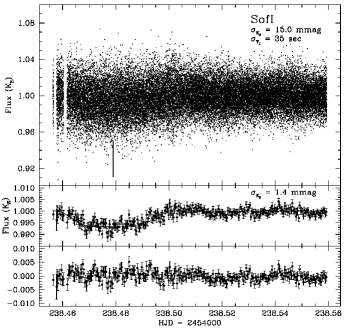
Figure 1: Photometry of the GJ 436b transit obtained with SofI. Top panel: the normalized light curve, with a integration time of 0.239 sec. The central time of the transit is marked at HJD $2454238.47898$. Error-bars are omitted for the sake of clarity. The out-of-transit r.m.s. flux on the unbinned curve ($\sigma_{K_{S}}$), and the timing error ($\sigma_{T_{C}}$) are also shown. Middle panel: the binned curve, and the best fitting model. The bin width is 30 sec. Error bars represent the flux r.m.s. within each bin. Note the different Y-axis range on the panels. The out-of-transit r.m.s. flux ($\sigma_{K_{S}}$) of the binned curve is also presented. Bottom panel: The residuals of the best fitting model to the binned curve.

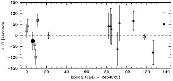
Figure 2: The observed minus calculated time-of-transit diagram for the different timing values in the literature, as a function of the observed epoch, for GJ 436b. Different symbols represent different literature sources. The open squares are from Shporer et al. (2008). The open triangle is an average of the value from Gillon et al. (2007a), Deming et al. (2007), and Southworth (2008), with the corrections given by Bean et al. (2008). The solid triangles are from Bean & Seifahrt (2008). The open circle is from Alonso et al. (2008). The solid squares come from Ribas et al. (2009). Finally, our timing estimate is drawn with a solid circle at $E=6$. All measurements are listed in Table 3

Many follow-up observations of GJ 436b has been carried out with both Spitzer Space Telescope (Gillon et al. 2007a; Deming et al. 2007; Demory et al. 2007; Southworth 2008) and the Hubble Space Telescope (Bean & Seifahrt 2008), and recently ground based observations have given a timing precision comparable to space based observations (Alonso et al. 2008; Shporer et al. 2008). They are all listed in Table 3.

Considering the newest literature data, and our measurement we recalculated the ephemeris of GJ 436b by fitting a weighted linear relation, to obtain a period $P=2.6438986\pm 0.0000016$ d, and a “zero transit” epoch $T_{C}(E=0)=2454222.61588\pm 0.00012$ HJD. The new epoch presented in this work is in excellent agreement with these ephemeris, and they in turn agree with those of Ribas et al. (2009), and Bean & Seifahrt (2008). Figure 2 shows the residuals of the fit of the new ephemeris as a function of the observed epoch for the available timing values in the literature, and our timing value at epoch $E=6$.

The data show some TTVs of up to 98 sec. – smaller than the predicted deviations of order of a few minutes for a 1-10 Earth mass companion on a resonant 2:1 orbit (Alonso et al. 2008). However, this deviations are consistent with zero, within their respective uncertainties. Further observations with higher accuracy are necessary to constrain better the properties of this system and to address the question if it bears other planets.

Table 3: GJ 436b timing measurements.

$T_{C}$ (HJD)	$\sigma_{T_{C}}$ (d)	Epoch	Reference
2454222.61612	0.00037	0	(1)
2454225.26029	0.00038	1	(1)
2454238.47898	0.00040	6	This work
2454243.76657	0.00026	8	(1)
2454246.40982	0.00040	9	(1)
2454251.69956	0.00030	11	(1)
2454280.78165	0.00017	22	(2,3,4)
2454439.41607	0.00068	82	(5)
2454444.70385	0.00093	84	(5)
2454447.34757	0.00080	85	(5)
2454463.20994	0.00089	91	(5)
2454468.49911	0.00094	93	(5)
2454505.51379	0.00050	107	(6)
2454534.59584	0.00015	118	(7)
2454558.39010	0.00063	127	(6)
2454587.47447	0.00061	138	(6)

References: (1) - Shporer et al. (2008); (2) - Gillon et al. (2007a); (3) - Deming et al. (2007); (4) - Southworth (2008); (5) - Bean & Seifahrt (2008); (6) - Ribas et al. (2009); (7) - Alonso et al. (2008).

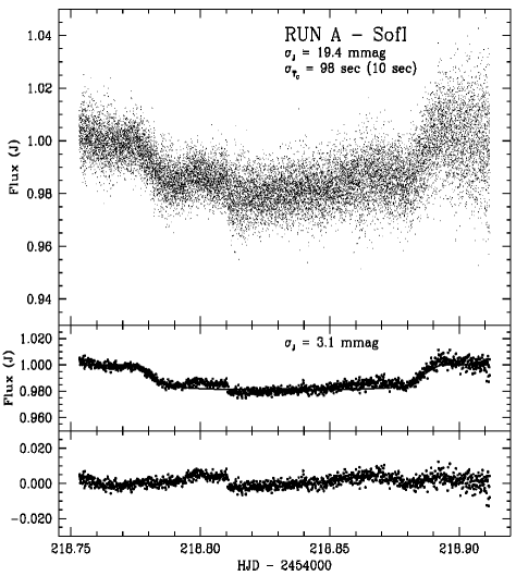
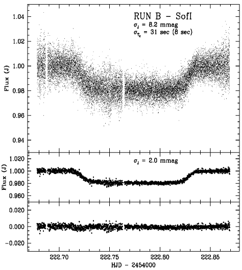
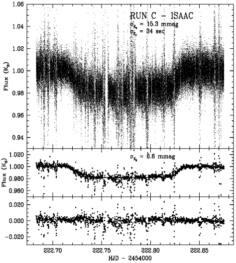
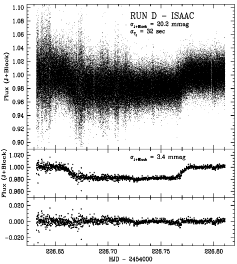
Figure 3: Photometry of the XO-1b transits obtained with SofI and ISAAC. Each panel shows (from top to bottom) the original light curve with a 10 sec bin size version with the best-fitting model, and the residuals of the fit. Top-left panel: Run A, observed with SofI, in the $J$ band. Top-right panel: Run B, observed with SofI, in the $J$ band. Bottom-left panel: Run C, observed with ISAAC, in the $K_{S}$ band. Bottom-right panel: Run D, observed with ISAAC, in the $J$+Block band. Each panel gives the out-of-transit r.m.s. flux of the unbinned curve (upper sub-panel), and of the binned curve (middle sub-panel). The timing error ($\sigma_{T_{C}}$) for each transit is printed. Note that for runs A and B we also give, in brackets, the timing error obtained if only the ingress-egress phases are considered. See more details in Sect. 3.2

3.2 XO-1b

The XO-1b light curves were analyzed in a similar way as for GJ 436b. The quadratic stellar limb-darkening coefficients utilized here were: $a=0.00592$ and $b=0.34954$ for the $K_{S}$ light curve, and $a=0.10923$ and $b=0.35938$ for the $J$+Block light curve.

After fixing the system parameters we calculated the transit midpoint for the 4 light curves separately. The errors were calculated with the same bootstrapping technique described above. The transit timings calculated here are shown in Table 4.

Interestingly, the uncertainties of the runs A and B decrease significantly, if the $\chi^{2}$ is calculated only over the ingress and the egress phases: 0.00012 d and 0.00009 d (10 and 8 sec), respectively. The bootstrapping simulation was also done over these parts of the light curve. Apparently, using only the ingress and egress excludes some of the systematic effects that occurred during the rest of the transit, and were reflected in the error distribution. Therefore, we consider the errors given in Table 4 to be upper limits of the uncertainties. The errors of the Runs C and D remained virtually unchanged: 0.00044, in both cases, most likely because they were obtained in poor weather conditions and the errors are dominated by the reduction of flux during the periods of poor atmospheric transmission.

Table 4: XO-1b timing measurements.

$T_{C}$ (HJD)	$\sigma_{T_{C}}$ (d)	Epoch	Reference
2453127.03850	0.00580	-173	(1)
2453142.78180	0.02180	-169	(1)
2453150.68550	0.01060	-167	(1)
2453154.62500	0.00260	-166	(1)
2453158.56630	0.00340	-165	(1)
2453162.51370	0.00250	-164	(1)
2453166.45050	0.00250	-163	(1)
2453170.39170	0.00370	-162	(1)
2453229.51430	0.00450	-147	(1)
2453237.40430	0.00320	-145	(1)
2453241.34100	0.00670	-144	(1)
2453808.91700	0.00110	0	(2)
2453875.92305	0.00036	17	(3)
2453879.86400	0.00110	18	(3)
2453883.80565	0.00019	19	(3)
2453887.74679	0.00016	20	(3)
2454218.83331	0.00114	104	This work (A)
2454222.77539	0.00036	105	This work (B)
2454222.77597	0.00039	105	This work (C)
2454226.71769	0.00037	106	This work (D)

References: (1) - Wilson et al. (2006); (2) - McCullough et al. (2006); (3) - Holman et al. (2006).

The final light curves are shown in Fig. 3, with a 20 sec bin width version to easily show the best fitting model. Run A shows some systematics that could not be corrected, so this curve was only used to get timing value, and not planetary parameters.

We fitted a weighted linear relation to the timing values listed in Table 4, to get the predicted ephemeris for the transits of XO-1b. This new ephemeris correct the long term difference in the ephemeris given by McCullough et al. (2006) and Wilson et al. (2006). Our fit gives us: $P=3.9415128\pm 0.0000028$ d, and a “zero transit” epoch $T_{C}(E=0)=2453808.91682\pm 0.00013$ HJD. In this calculation, we use the weighted average of runs B, and C, which spans the same epoch. This calculations are shown in Fig. 4. Note that runs C and D, carried out with the bigger telescope, but under worse weather conditions yield less accurate timing measurements than transits observed with the smaller telescope but under better weather conditions (i.e. run B), demonstrating the impact of the weather on the high precision photometry required to detect the transiting planets.

The amplitude of the resulting TTVs, show no evidence for a perturbing third body in the system, in agreement with the results of Holman et al. (2006).

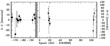
Figure 4: The observed minus calculated time-of-transit diagram for the different timing values in the literature, as a function of the observed epoch for XO-1b. For clarity the diagram was divided in two different scale panels (minutes in the left panel, and seconds in the right panel). Different symbols represents different literature sources. The pentagons are from Wilson et al. (2006). The squares are the values from Holman et al. (2006). The open triangle is the value from McCullough et al. (2006). Our timing values are shown with solid triangles. All measurements are listed in Table 4.

4 Conclusions

Here, we present new ground based high cadence near-infrared observations of one transit of the hot-Neptune GJ 436b, and four transits, spanning three epochs, of the hot-Jupiter XO-1b.

We achieve transiting timing accuracies of about 30 sec for individual transits. The uncertainty is dominated by systematic effects, and greatly exceeds the few second errors predicted by photon noise dominated observations. We find no significant evidence for perturbations of the orbital motion of GJ 436b nor XO-1b by other bodies in the system. Of course, a proper test of this hypothesis will require monitoring of multiple transits with the same or even higher accuracy.

We demonstrate that the ground-based high-cadence observations of transiting extrasolar planets is an excellent technique for constraining the parameters of extrasolar planetary systems because of the statistical significance of the obtained timing measurements. The timing precision is comparable with the space-based observations, making this method a good alternative to the space mission with their high cost and limited life-time.