About the temperature of moving bodies

Abstract.

Relativistic thermodynamics is constructed from the point of view of special relativistic hydrodynamics. A relativistic four-current for heat and a general treatment of thermal equilibrium between moving bodies is presented. The different temperature transformation formulas of Planck and Einstein, Ott, Landsberg and Doppler appear upon particular assumptions about internal heat current.

1. Introduction

Considering the temperature of moving bodies, the easier question is to answer, what is the apparent spectral temperature. In this case a spectral parameter is transformed if the thermalized source is moving with respect to the observer (detector system), and the transformation rule can be derived from that of the energy and momentum in the co-moving system.

This has been known from the beginnings of the theory of special relativity and never has been seriously challenged. An essentially tougher problem is to understand the relativistic thermalization: what is the intensive parameter governing the state with energy exchange equilibrium between two, relatively moving bodies in the framework of special relativity. In particular how this general temperature should transform and how does it depend on the speed of the motion. Here several answers has been historically offered, practically including all possibilities.

Planck and Einstein concluded that moving bodies are cooler by a Lorentz factor [1, 2, 3], first Blanus̆a then Ott has challenged this opinion [4, 5] by stating that on the contrary, such bodies are hotter by a Lorentz factor. During later disputes several authors supported one or the other view (see e.g. [6, 7, 8, 9, 10, 11, 12, 13] and the references therein) and also some new opinions emerged. Landsberg argued for unchanged values of the temperature [14, 15]. Other authors observed that for a thermometer in equilibrium with black body radiation the temperature transformation is related to the Doppler formula [16, 17, 18, 19, 20], therefore the measured temperature seems to depend on the physical state of the thermometer. This problem is circumvented by the suggestion that thermal equilibrium would have a meaning only in case of equal velocities [21, 22, 23].

Behind these different conclusions there are, in our opinion, different views about the energy transfer and mechanical work, and the identification of the heat [12]. In a simplifying manner the assumptions and views about the Lorentz transformation properties of internal energy, work, heat, and entropy influence such properties and the very definition of the absolute temperature. Coming to the era of fast computers, a renewed interest emerged in such questions by modelling stochastic phenomena at relativistic energy exchanges and relative speeds [24, 25, 26]. In particular, dissipative hydrodynamics applied to high energy heavy ion collisions requires the proper identification of temperature and entropy [27, 28, 29, 30, 31, 32, 33, 34, 35]. In this letter we show that our approach to replace the Israel-Stewart theory of dissipative hydrodynamics, proposed earlier [36, 37, 38, 39], is related to the problem of thermalization of relatively moving bodies with relativistic velocities and our suggestion is compatible with the foundations of thermodynamics and guarantees causal heat propagation.

oø

By doing so we encounter the following questions in our analysis:

1. What moves (or flows)? Total energy and momentum do flow correlated, but further conserved charges (baryon number, electric charge, etc.) may flow differently. In relativistic systems one has to deal with the possibility that the velocity field is not fixed to either current, not being restricted to the Landau-Lifshitz [40] or Eckart [41] frames.

2. What is a body? We exploit, how do integrals over extended volumes relate to the local theory of hydrodynamics, and what is a good local definition for volume change in relativistic fluids. In close relation to this, we suggest a four-vector generalization to the concept of heat.

3. What is a proper equation of state? Here the functional dependency between entropy and the relativistic internal energy is fixed to a particular form.

4. What is the proper transformation of the temperature? As we have mentioned above prominent physicists expressed divergent opinions on this in the past. This problem is intimately related to that of thermal equilibrium and to the proper description of internal energy.

2. Hydro- and thermodynamics

In this letter we concentrate on the energy-momentum density of a one-component fluid, but the results can be generalized considering conserved currents in multi-component systems easily. The energy-momentum tensor can be split into components aligned to the fiducial four-velocity field, $u^{a}(x)$, and orthogonal ones:

(1) $$T^{ab} = eu^{a}u^{b}+u^{a}q^{b}+q^{a}u^{b}+P^{ab}$$

with $u_{a}q^{a}=0$ and $u_{a}P^{ab}=P^{ab}u_{b}=0$. When considering complex systems, like a quark-gluon plasma, the velocity field can be aligned only with one of the conserved currents, unless several currents are parallel (i.e. different conserved charges are fixed to the same carriers). In our present treatment the velocity field is general.

Relativistic thermodynamics is obtained by integrating the local energy-momentum conservation on a suitably defined extended and homogeneous thermodynamic body. Therefore in the balance of energy-momentum we separate the terms perpendicular and parallel to the velocity field as

(2) $$\partial_{b}T^{ab} = \frac{d}{d\tau}({e}u^{a}+{q}^{a})+(eu^{a}+q^{a})\partial_{b}u^{b}$$

$$+ p(\frac{d}{d\tau}u^{a}+u^{a}\partial_{b}u^{b})-\frac{du_{b}}{d\tau}(u^{a}q^{b}+\Pi^{ab})$$

$$- \nabla^{a}p+\nabla_{b}(u^{a}q^{b}+\Pi^{ab})=0^{a}.\ \ \$$

From now on the proper time derivative is denoted by a dot $\dot{f}=df/d\tau=u_{a}\partial^{a}f$ for an arbitrary function $f(x)$. $\nabla^{a}=\partial^{a}-u^{a}u_{c}\partial^{c}$ denotes a derivative perpendicular to the velocity field and we also split the pressure tensor into a hydrostatic part and a rest: $P^{ab}=p(u^{a}u^{b}-g^{ab})+\Pi^{ab}$.

Let us now assume, that $u^{a}$ is smooth and we may give a connected smooth surface $H$ that is initially perpendicular to the velocity field and has a smooth (two -dimensional) boundary. As a further simplification we will assume that the velocity field is not accelerating $\dot{u}^{a}=0^{a}$, therefore $\partial_{a}u^{a}=\nabla_{a}u^{a}$ and the hypersurface remains perpendicular to the four-velocity field. Hence the propagation of the surface can be characterized by the proper time $\tau$ of any of its wordlines. We refer to this hypersurface - a three dimensional spacelike set related to our fluid - as a thermodynamic body. Considering homogeneous bodies we set $\nabla_{a}e=0$ and $\nabla_{a}p=0$. It is important that the velocity field itself is not homogeneous, $\nabla^{a}u^{b}\neq 0$. Now integration of (2) on $H(\tau)$ results in

$$\int_{H(\tau)}(\dot{e}u^{a}+\dot{q}^{a}+(eu^{a}+q^{a})\partial_{b}u^{b}+pu^{a}\partial_{b}u^{b})dV\!=\!\!$$

(3) $$\int_{H(\tau)}\nabla_{b}(u^{a}q^{b}\!+\Pi^{ab})dV.$$

With the above conditions wa apply the transport theorem of Reynolds to the l.h.s. of eq.(3) and the Gauss-Ostrogradsky theorem to the r.h.s. of eq.(3) and obtain

(4) $$\dot{E}\bar{u}^{a}+\dot{G}^{a}+p\bar{u}^{a}\dot{V}=\oint_{\partial H(\tau)}\limits\!\!\!\left(u^{a}q^{b}\!+\Pi^{ab}\right)\,dA_{b}=\delta Q^{a}.$$

Here $\bar{u}^{a}=\int_{H}u^{a}dV/V$ is the average velocity field inside $H$, $E=eV$ is the total energy, $G^{a}=\int_{H}q^{a}dV,$ and $dA_{b}$ is the two-form surface measure circumventing the homogeneous body in the region $H(\tau)$. The two-dimensional surface integral term is the physical energy and momentum leak (dissipation rate) from the body under study, we denote it by $\delta Q^{a}$. This is a four-vector generalization of the concept of heat. It describes both energy and momentum transfers to or from the homogeneous body.

The derivation of the temperature in thermodynamics is related to the maximum of the total entropy of a system (under various constraints). This way its reciprocal, $1/T$ is an integrating factor to the heat in order to obtain a total differential of the entropy [42, 43]. Here we follow the same strategy considering a vectorial integrating factor $A^{a}$:

(5) $$\delta Q^{a}=\dot{E^{a}}+p\bar{u}^{a}\dot{V}=A^{a}\dot{S}+\Sigma^{a}$$

with ${E}^{a}=E\bar{u}^{a}+G^{a}$ the energy-momentum vector of the body, $\dot{\bar{u}}^{a}=0$ and $\Sigma^{a}$ orthogonal to $A^{a}$. The decisive point is, that – according to the above – the entropy of the homogeneous body is a function of the energy-momentum vector and the volume: $S=S(E^{a},\text{V})$. Multiplying eq.(5) by $A_{a}d\tau/(A_{b}A^{b})$ and utilizing that $d\bar{u}^{a}=0$ we obtain

(6) $$dS=\frac{A_{a}\bar{u}^{a}}{A_{b}A^{b}}\,dE+\frac{A_{a}}{A_{b}A^{b}}\,dG^{a}+p\frac{A_{a}\bar{u}^{a}}{A_{b}A^{b}}\,d\text{V}.$$

The connection to classical thermodynamics is best established by the temperature definition

(7) $$\frac{1}{T}:=\frac{A_{a}\bar{u}^{a}}{A_{b}A^{b}}.$$

The intensive parameter associated to the change of the four-vector $G^{a}$ is denoted by

(8) $$\frac{g^{a}}{T}:=\frac{A^{a}}{A_{b}A^{b}}.$$

With these notations we arrive at the following form of the Gibbs relation:

(9) $$TdS=dE+g_{a}dG^{a}+pdV.$$

Due to the definitions eq. (7,8) $g_{a}\bar{u}^{a}=1$. Hence the Gibbs relation can be written in the alternative form

(10) $$TdS=g_{a}\,dE^{a}+pdV,$$

suggesting that the traditional change of the energy, $dE$, has to be generalized to the change of the total energy-momentum four-vector, $dE^{a}=d(E\bar{u}^{a}+G^{a}).$

For the well-known Jüttner distribution [44] $g^{a}=\bar{u}^{a}$. This equality has been postulated among others in the classical theory of Israel and Stewart [45]. Then (10) reduces to

(11) $$TdS=d\tilde{E}+pdV,$$

where $\tilde{E}=\bar{u}_{a}E^{a}$. In this case the internal energy can be interpreted as $\tilde{E}$, but its total differential contributes to the Gibbs relation. In the general case $g^{a}\neq\bar{u}^{a}$ - considered below - there remains a term, related to momentum transfer. It is reasonable to assume that the new intensive variable is timelike: $g_{a}g^{a}\geq 0$. Then we introduce

(12) $$w^{a}:=g^{a}-\bar{u}^{a}.$$

Now $\|w^{a}\|^{2}=-w^{a}w_{a}=-g^{a}g_{a}+1{\leq}1$ follows. The spacelike four-vector $w^{a}$ has the physical dimension of velocity. Due to $-1\leq w^{a}w_{a}\leq 0$ and $\bar{u}_{a}w^{a}=0$ its general form is given by $w^{a}=(\gamma v|{\mathbf{w}}|,\gamma{\mathbf{w}})$. In this case $|{\mathbf{w}}|^{2}\leq 1$. We interpret $\mathbf{w}$ as the velocity of the internal energy current.

Here some important physical questions arise: is it only a single or several differential terms describing the change of energy and momentum? When two, relatively moving bodies come into thermal contact what can be exchanged among them in the evolution towards the equilibrium?

3. Two bodies in equilibrium

Let us now consider two different bodies with different average velocities and energy currents. When all components of $E^{a}$ and the total volume are kept constant independently, i.e. $dE^{a}_{1}+dE_{2}^{a}=0$ and $dV_{1}+dV_{2}=0$ while $dS(E_{1}^{a},V_{1})+dS(E_{2}^{a},V_{2})=0$ in the entropy maximum, then from (10) we obtain the conditions

(13) $$\frac{g^{a}_{1}}{T_{1}}=\frac{g^{a}_{2}}{T_{2}},\qquad\frac{p_{1}}{T_{1}}=\frac{p_{2}}{T_{2}}.$$

This, in general, does not mean the equality of temperatures.

In order to simplify the discussion we restrict ourselves to one-dimensional motions and consider $\bar{u}^{a}=(\gamma,\gamma v)$ with $\gamma=1/\sqrt{1-v^{2}}$ Lorentz-factors. The energy current velocity is given by $w^{a}=(\gamma vw,\gamma w)$ and $q^{a}={(\gamma(1+vw)},{\gamma(v+w))}$. Here $w$ describes the speed of internal energy current. The thermal equilibrium condition (13) hence requires

$$\frac{\gamma_{1}(1+v_{1}w_{1})}{T_{1}} = \frac{\gamma_{2}(1+v_{2}w_{2})}{T_{2}},$$

(14) $$\frac{\gamma_{1}(v_{1}+w_{1})}{T_{1}} = \frac{\gamma_{2}(v_{2}+w_{2})}{T_{2}}.$$

The ratio of these two equations reveals that in equilibrium the composite relativistic velocities are equal,

(15) $$\frac{v_{1}+w_{1}}{1+v_{1}w_{1}}=\frac{v_{2}+w_{2}}{1+v_{2}w_{2}},$$

and the difference of their squares leads to

(16) $$\frac{\sqrt{1-w_{1}^{2}}}{T_{1}}=\frac{\sqrt{1-w_{2}^{2}}}{T_{2}}.$$

The equality of some other velocities were investigated by several authors [21, 22, 23, 46].

One realizes that in the thermal equilibrium condition four velocities are involved for a general observer: $v_{1}$, $v_{2}$, $w_{1}$ and $w_{2}$. By a Lorentz transformation only one of them can be eliminated. The remaining three (relative) velocities reflect physical conditions in the system. According to eq.(15)

(17) $$w_{1}=\frac{v+w_{2}}{1+vw_{2}}$$

with $v=(v_{2}-v_{1})/(1-v_{1}v_{2})$ relative velocity. The associated factor, $\sqrt{1-w_{1}^{2}}$ can be expressed and the temperatures satisfy

(18) $$T_{1}=T_{2}\,\frac{\sqrt{1-v^{2}}}{1+vw_{2}}.$$

This includes the general Doppler formula [16, 17, 18, 19, 20, 47].

It is enlightening to investigate this formula with different assumptions about the energy current speed in the observed body, $w_{2}$. The induced energy current speed in an ideal thermometer, $w_{1}$ and the temperature it shows, $T_{1}$, are now determined by eqs.(17) and (18). Figure 1 plots temperature ratios $T_{1}/T_{2}$ for a body closing with $v=-0.6$ as a function of the energy current speed, $w_{2}$.

1. $w_{2}=0$: the current stands in the observed body. In this case $w_{1}=v$, the measured energy current speed is that of the moving body, and $T_{1}=T_{2}\sqrt{1-v^{2}}<T_{2}$, the moving body appears cooler by a Lorentz factor [1, 3, 2] (see Fig 2).

2. $w_{1}=0$: the current stands in the thermometer. In this case we must have $w_{2}=-v$ and $T_{1}=T_{2}/\sqrt{1-v^{2}}>T_{2}$, the moving body appears hotter [4, 5, 7, 12] (see Fig 3).

3. $w_{1}+w_{2}=0$: the current is standing in the total system of moving body and thermometer, the individual contributions exactly compensate each other. This is achieved by a special value of the energy current velocities, $w_{2}=-w$, $w_{1}=w$ with $w=(1-\sqrt{1-v^{2}})/{v}$. In this case even the apparent temperatures are equal, $T_{1}=T_{2}$ [14, 15] (see Fig 4).

4. $w_{2}=1$: a radiating body (e.g. a photon gas) is moving. In this case $w_{1}=1$, and one obtains $T_{1}=T_{2}\sqrt{\frac{1-v}{1+v}}$. It means that $T_{1}<T_{2}$ for $v>0$, a Doppler red shifted temperature is measured for an aparting body (see Fig 5) - quite common for astronomical objects - and $T_{1}>T_{2}$ for $v<0$, a Doppler blue shifted temperature appears for closing bodies - more common in high energy accelerator experiments.

On figures (2)-(5) we fix the reference frame to the thermometer, therefore $u_{1}^{a}=(1,0)$ (the vertical axis is time). The energy current velocity four-vectors are perpendicular to the corresponding four-velocities, therefore they are on lines symmetrical to the light cones. The four-velocity vectors end on the timelike hyperbolas and the spacelike energy current velocities end inside the spacelike hyperbolas. The temperature ratios are determined by the magnitudes of the $g^{a}$-s as $T_{1}/T_{2}=\|g_{1}^{a}\|/\|g_{2}^{a}\|$ (see [48].

4. Lorentz scalar temperature

According to the classical ansatz $g^{a}=\bar{u}^{a}$, the total entropy has to depend on the total energy $E=\bar{u}_{a}{E}^{a}$. Then the equilibrium conditions (17) and (18) result in zero relative velocity $v=0$ and the temperatures are equal $T_{1}=T_{2}$.

However, thermodynamic and generic stability considerations are favoring an other Lorentz-scalar combination $\|{E}\|=\sqrt{{E}_{a}{E}^{a}}$ [36, 37, 38, 39]. Denoting the partial derivative of entropy $S(\|E\|,V)$ with respect to its first argument by $1/\theta=\frac{\partial S}{\partial\|E\|}$, one re-writes the total differential,

(19) $$dS=\frac{1}{\theta}d\|E\|+\frac{\tilde{p}}{\theta}dV=\frac{g_{a}}{T}dE^{a}+\frac{p}{T}dV,$$

and comparing to the general Gibbs relation (10) one obtains the correspondence

(20) $$\frac{g^{a}}{T}=\frac{1}{\theta}\frac{E^{a}}{\|E\|},\qquad\frac{p}{T}=\frac{\tilde{p}}{\theta}.$$

It follows that the length of the intensive four-vector, $g^{a}$, is the ratio of the traditional (energy associated) and scalar (energy-momentum four-vector length associated) temperatures: $\sqrt{g_{a}g^{a}}=T/\theta$. On the other hand its projection to the average velocity reveals the value in the comoving system:

(21) $$g_{a}\bar{u}^{a}=\frac{T}{\theta}\,\frac{E_{a}\bar{u}^{a}}{\|E\|}=1.$$

This equation relates the energy-momentum-associated scalar temperature, $\theta$ to the energy-associated one, $T$. As a consequence we obtain

(22) $${g^{a}}=\frac{E^{a}}{E^{b}\bar{u}_{b}},\qquad{w^{a}}=\frac{E^{a}-\bar{u}^{a}(E^{b}\bar{u}_{b})}{E^{c}\bar{u}_{c}}.$$

The later formula clearly interpret $w^{a}$ as the quotient of the comoving, average velocity related energy current (momentum) and energy of the thermodynamic body, that is the energy current velocity.

Finally we remark, that in the simple two dimensional particular case we obtain that $\theta=T/\sqrt{1-w^{2}}$. Therefore the equilibrium condition (16) gives equal scalar temperatures: $\theta_{1}=\theta_{2}$. This is a stronger reflection of Landsberg’s view, and his physical arguments in [14, 15] than the assumption of zero total energy current velocity.

Figure 1. Ratio of the temperatures of the observed body in its rest frame, $T_{2}$ to that shown by an ideal thermometer, $T_{1}$ as a function of the the speed of the heat current in the body, $w_{2}$ while approaching with the relative velocity $v=-0.6$.

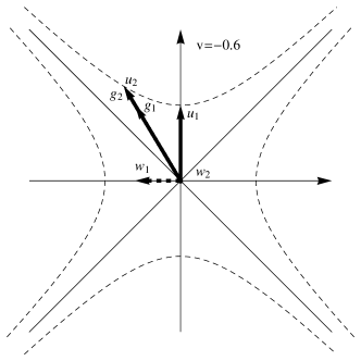
Figure 2. The space-time figure for the Planck-Einstein rule of two thermodynamic bodies in equilibrium. There is no energy current in the observed body ($w^{a}_{2}=0$), therefore the $u^{a}_{2}$ four-velocity (solid arrow) is parallel to the vectors ($g^{a}_{1},g^{a}_{2}$). The ratio of the temperatures is $T_{1}/T_{2}<1$.

Figure 3. The space-time figure for the Blanuša-Ott rule. The energy current stands in the thermometer ($w^{a}_{1}=0$), therefore the $u^{a}_{1}$ four-velocity (solid arrow) is parallel to the vectors ($g^{a}_{1},g^{a}_{2}$). The ratio of the temperatures is $T_{1}/T_{2}>1$.

Figure 4. The space-time figure for the Landsberg rule. There is no energy current in the composed system, therefore the four-vectors ($g^{a}_{1}$, $g^{a}_{2}$, dotted arrows) are equal. The ratio of temperatures is $T_{1}/T_{2}=1$. Here $w_{1}=-0.33$, $w_{2}=0.33$.

Figure 5. The space-time figure for the Doppler red shift rule of two thermodynamic bodies in equilibrium. The energy current speed (dashed arrows) in the observed body is that of the light $w_{2}=1$, therefore $w_{1}=1$, and the four-vectors of energy-momentum intensives ($g^{a}_{1}$, $g^{a}_{2}$, dotted arrows) are light-like.

5. Summary

We investigated the possible derivation of basic thermodynamical laws for homogeneous bodies from relativistic hydrodynamics. The dependence of entropy on internal energy is replaced by a dependence on the energy-momentum four-vector, $E^{a}$. As a novelty a relativistic heat four-vector has been formulated. For the traditional, energy exchange related temperature, $T$, a universal transformation formula is obtained. For a general observer four velocities are involved in the equilibrium condition of two thermodynamic bodies in equilibrium. One of them can be eliminated by choosing the observing frame, the physical relation depends only on the relative velocity. Another condition connects the internal heat currents in the bodies in thermal contact. So there remains two velocity like parameters to describe thermal equilibrium: the energy current speed (the velocity related to the integrated internal heat current density) in one of the bodies and their relative velocity. The traditional temperature transformation formulas belong to corresponding particular choices on the energy current speeds. This can be the reason that no agreement could be achieved historically. For most common cases there is no heat current in the observed body but it flows in the thermometer. This leads to the Planck-Einstein transformation formula.

The closer relation to dissipative hydrodynamics favors a particular dependence of entropy on energy-momentum and leads to a Lorentz scalar temperature.

Our approach is covariant, and the compatibility to hydrodynamics clarifies that the Planck-Ott imbroglio is not a problem of synchronization as it was supposed in [49, 25]. It makes possible to interpret the classical paradoxical results of Planck and Einstein, Ott, Landsberg and Doppler in a unified treatment. Our investigations reveal that despite of the apparent paradoxes related to Lorentz transformations, there is a covariant relativistic thermodynamics with proper absolute temperature in full agreement with relativistic hydrodynamics.

6. Acknowledgement

The authors thank to L. Csernai for his enlighting remarks.

References

- [1] M. Planck. Zur Dynamik bewegter Systeme. Sitzungsberichten der königliche Preussen Akademie der Wissenschaften, pages 542–570, 1907.
- [2] A. Einstein. Über das Relativitätsprinzip und die aus demselben gezogenen Folgerungen. Jahrbuch der Radioaktivität und Elektronik, 4:411–462, 1907.
- [3] M. Planck. Zur Dynamik bewegter Systeme. Annalen der Physik, 331(6):1–34, 1908.
- [4] D. Blanuša. Sur les paradoxes de la notion d’énergie. Glasnik mat. fiz.; astr., 2(4-5):249–50, 1947.
- [5] H. Ott. Lorentz-Transformation der Wärme und der Temperatur. Zeitschrift für Physik, 175:70–104, 1963.
- [6] J. H. Eberly and A. Kujawski. Relativistic statistical mechanics and blackbody radiation. Physical Review, 155(1):10–19, 1967.
- [7] D. Ter Haar and H. Wergeland. Thermodynamics and statistical physics in the special theory of relativity. Physics Reports, 1(2):31–54, 1971.
- [8] Von H.-J. Treder. Die Strahlungs-Temperatur bewegter Körper. Annalen der Physik, 7(34/1):23–29, 1977.
- [9] C. Møller. The theory of relativity. The international series of monographs in physics. Oxford University Press, Delhi-Bombay- Calcutta-Madras, 2nd edition, 1972.
- [10] R.G. Newburgh. Comments on the derivation of the Ott relativistic temperature. Physics Letters A, 78.
- [11] I-Shih Liu. On entropy flux-heat flux relation in thermodynamics with Lagrange multipliers. Continuum Mechanics and Thermodynamics, 8:247–256, 1996.
- [12] M. Requardt. Thermodynamics meets special relativity - or what is real in physics? 2008. arXiv:0801.2639v1[gr-qc].
- [13] G. L. Sewell. On the question of temperature transformations under Lorentz and Galilei boosts. Journal of Physics A: Mathematical and General, 41:382003, 2008.
- [14] P. Landsberg. Does a moving body appears cool? Nature, 212:571–573, 1966.
- [15] P. Landsberg. Does a moving body appears cool? Nature, 214:903–4, 1967.
- [16] S. S. Costa and G. E. A. Matsas. Temperature and relativity. Physics Letters A, 209:155–159, 1995.
- [17] P. Landsberg and G. E. A. Matsas. Laying the ghost of the relativistic temperature transformation. Physics Letters A, 223:401–403, 1996.
- [18] P. Landsberg and G. E. A. Matsas. The impossibility of a universal relativistic temperature transformation. Physica A, 340:92–94, 2004.
- [19] J. Casas-Vázquez and D. Jou. Temperature in non-equilibrium states. Reports on Progress in Physics, 66:1937–2023, 2003.
- [20] D. Mi, Hai Yang Zhong, and D. M. Tong. There exist different proposals for relativistic temperature transformation: the whys and wherefores. Modern Physics Letters A, 24(1):73–80, 2009.
- [21] N. G. van Kampen. Relativistic thermodynamics of moving systems. The Physical Review, 173:295–301, 1968.
- [22] P. T. Landsberg. Thermodynamics and Statistical mechanics. Oxford Clarendon Press, Oxford, 1978.
- [23] D. Eimerl. On relativistic thermodynamics. Annals of Physics, 91:481–498, 1975.
- [24] D. Cubero, J. Casado-Pascual, J. Dunkel, P. Talkner, and P. Hänggi. Thermal equilibrium and statistical thermometers in special relativity. Physical Review Letters, 99:170601, 2007.
- [25] J. Dunkel and P. Hänggi. Relativistic Brownian motion. Physics Reports, 471(1):1–73, 2009. arXiv:0812.1996v2.
- [26] A. Montakhab, M. Ghodrat, and M. Barati. Statistical thermodynamics of a two-dimensional relativistic gas. Physical Review E, 79:031124, 2009.
- [27] A. Muronga. Causal theories of dissipative relativistic fluid dynamics for nuclear collisions. Physical Review C, 69:0304903(16), 2004.
- [28] T. Koide, G. S. Denicol, Ph. Mota, and T. Kodama. Relativistic dissipative hydrodynamics: a minimum causal theory. Physical Reviews C, 75(3):034909(10), 2007. hep-ph/0609117.
- [29] G. S. Denicol, T. Kodama, T. Koide, and Ph. Mota. Extensivity of irreversible current and stability in causal dissipative hydrodynamics. Journal of Physics G - Nuclear and Particle Physics, 36(3):035103, 2009. arXiv:0808.3170.
- [30] R. Baier and P. Romatschke. Causal viscous hydrodynamics for central heavy-ion collisions. European Physical Journal C, 51(3):677–687, 2007. nucl-th/0610108.
- [31] T. Osada and G. Wilk. Nonextensive hydrodynamics for relativistic heavy-ion collisions. Physical Review C, 77:044903, 2008. arXiv:0710.1905.
- [32] E. Dumitru, E. Molnár, and Y. Nara. Entropy production in high-energy heavy-ion collisions and the correlation of shear viscosity and thermalization time. Physical Review C, 76(2):024905, 2007. arXiv:0807.0544.
- [33] D. Molnár and P. Huovinen. Dissipative effects from transport and viscous hydrodynamics. Journal of Physics G, 35(10):104125, 2008.
- [34] E. Molnár. Comparing the first and second order theories of relativistic dissipative fluid dynamics using the 1+1 dimensional relativistic flux corrected transport algorithm. Physical Review C, 60(3):413–429, 2009. arXiv:0807.0544.
- [35] H. Song and U. W. Heinz. Extracting the QGP viscosity from RHIC data - a status report from viscous hydrodynamics. Journal of Physics G, 36:064033, 2009. arXiv:0812.4274.
- [36] P. Ván and T. S. Bíró. Relativistic hydrodynamics - causality and stability. The European Physical Journal - Special Topics, 155:201–212, 2008. Zimányi’75 Workshop Proceedings, arXiv:0704.2039v2.
- [37] T. S. Bíró, E. Molnár, and P. Ván. A thermodynamic approach to the relaxation of viscosity and thermal conductivity. Physical Review C, 78:014909, 2008. arXiv:0805.1061 (nucl-th).
- [38] P. Ván. Internal energy in dissipative relativistic fluids. Journal of Mechanics of Materials and Structures, 3(6):1161–1169, 2008. Lecture held at TRECOP’07, arXiv:07121437 [nucl-th].
- [39] P. Ván. Generic stability of dissipative non-relativistic and relativistic fluids. Journal of Statistical Mechanics: Theory and Experiment, page P02054, 2009. arXiv: 0811.0257, SigmaPhy’08 Proceedings.
- [40] L. D. Landau and E. M. Lifshitz. Fluid mechanics. Pergamon Press, London, 1959.
- [41] Carl Eckart. The thermodynamics of irreversible processes, III. Relativistic theory of the simple fluid. Physical Review, 58:919–924, 1940.
- [42] H. B. Callen. Thermodynamics and an introduction to thermostatistics. John Wiley and Sons NY, New York, etc., 2nd edition, 1985.
- [43] T. Matolcsi. Ordinary thermodynamics. Akadémiai Kiadó (Publishing House of the Hungarian Academy of Sciences), Budapest, 2005.
- [44] F. Jüttner. Das maxwellsche gesetz der geschwindigkeitsverteilung in der relativtheorie. Annalen der Physik, 339(5):856–882, 1911.
- [45] W. Israel and J. M. Stewart. Progress in relativistic thermodynamics and electrodynamics of continuous media. In A. Helde, editor, General relativity and gravitation (One hundred years after the birth of Albert Einstein), volume 2, chapter 13, pages 491–525. Plenum Press, New York and London, 1980.
- [46] Chuang Liu. Is there a relativistic thermodynamics? A a case study of the meaning for special relativity. Studies in History and Philosophy of Science, 25(6):983–1004, 1994.
- [47] Marek Demia´nski. Relativistic astrophysics. PWN-Polish Scientific Publishers - Pergamon Press, Warszawa - Oxford, etc., 1985.
- [48] P. Ván and T. S. Bíró. Transformations of relativistic temperature - Planck-Einstein, Ott, Landsberg and Doppler formulas as particular cases. Wolfram Demonstration Project, 2009.
- [49] C. K. Yuen. Lorentz transformation of thermodynamic quantities. American Journal of Physics, 38(2):246–252, 1970.