Heavy-quark pair production in polarized photon-photon collisions at next-to-leading order: Fully integrated total cross sections

Abstract

We consider the production of heavy-quark pairs in the collisions of polarized and unpolarized on-shell photons and present, in analytic form, the fully integrated total cross sections for total photon spins $J_{z}=0,\pm 2$ at next-to-leading-order in QCD. Phenomenological applications include $b\bar{b}$ production, which represents an irreducible background to standard-model intermediate-mass Higgs-boson production, as well as $t\bar{t}$ production.

I Introduction

It has been emphasized by many physicists that running a future $e^{+}e^{-}$ linear collider (ILC) in the photon-photon mode is a very interesting option (see, e.g., Refs. proc95 ; badelek04 ). The high-energy on-shell photons can be generated by backward Compton scattering of laser light off the high-energy electron and positron bunches of the collider with practically no loss in energy and luminosity. In this respect, one of the most important reactions to consider is heavy-quark pair production in photon-photon collisions. A $\gamma\gamma$ collider becomes particularly important for studies of the standard-model Higgs boson when its mass is below the $W^{+}W^{-}$ production threshold. Then, the predominant decay is $H\to b\bar{b}$. The dominant background to this comes from $\gamma\gamma\to b\bar{b}$, which receives contributions from direct and resolved photons. We leave aside the latter for the time being and return to this in Sec. V. The use of longitudinally polarized photons of equal helicity (their angular momentum being $J_{z}=0$) suppresses this background by a factor of $m_{b}^{2}/s$ at the leading order in perturbation theory Haber ; Borden . Of course, the reason that the $J_{z}=0$ channel is important is that the Higgs signal comes entirely from it. Nevertheless, the above-mentioned suppression should not necessarily hold in general, since QCD higher-order corrections involve gluon emission, which permits the $b\bar{b}$ system to have $J_{z}\neq 0$. Therefore, the process of bottom-quark pair production in polarized-photon fusion would represent an irreducible background to intermediate-mass Higgs-boson production. Indeed, subsequent calculations of the next-to-leading-order (NLO) QCD corrections have confirmed these expectations KMC ; Jikia .

Furthermore, future photon colliders will become top-quark factories. The data obtained there, when combined with data on top-quark production from other reactions, will certainly improve our knowledge of the top-quark properties (see, e.g., Ref. hewett98 ). It should also be noted that the NLO corrections have a large effect on the threshold behavior and exhibit a peculiar spin dependence in this region.

Heavy-flavor production in photon-photon collisions receives contributions from direct and resolved incident photons. In the first case, photons behave as pointlike objects, interacting directly with the quarks in the hard scattering, while in the second case, the photon exhibits a complex structure involving quarks and gluons that participate in the hard interaction. In this paper, we present analytical results for the total cross sections for heavy-quark pair production by both polarized and unpolarized direct photons. The present work builds on the previous work of one of us KMC ; KM . In Ref. KMC , differential cross sections were calculated analytically in dimensional regularization DREG and cast into a very compact form. We note that this is the only publication where complete analytical results for polarized and unpolarized doubly differential cross sections are presented. In Ref. KM , top-quark pair production for energies not too far above threshold was studied, and the fully integrated result for the so-called “virtual plus soft” part of the cross section was derived. We also note that the results presented in the present work constitute the Abelian part of the gluon-induced hadroproduction of heavy-quark pairs.

This paper is organized as follows. Section II explains our notations. In Sec. III, we outline our general approach and discuss in detail our procedure and methodology. In Sec. IV, we present our analytically integrated total cross sections. Our conclusions are summarized in Sec. V. Finally, Appendix A elaborates on the calculation of one of the most difficult double integrals, Appendix B gives expressions for the various coefficient functions that appear in the main text, and Appendix C displays representations of our basis functions in terms of generalized Nielsen polylogarithms.

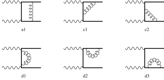
Figure 1: One-loop Feynman diagrams contributing to the photon-fusion amplitude. Wavy, curly, and solid lines represent photons, gluons, and heavy quarks, respectively

II Notation

For consistency, we closely follow the notations of Ref. KMC . The one-loop Feynman diagrams with $t$-channel topology relevant for heavy-flavor production by the scattering of two on-shell photons are depicted in Fig. 1. The $u$-channel diagrams are obtained from the depicted ones by crossing the incoming photon lines. Single-gluon radiation, which arises from the tree-level diagrams with a gluon attached in all possible ways to the heavy-quark line, contributes at the same order. We assign the four-momenta and helicities as

$$\gamma(p_{1},\lambda_{1})+\gamma(p_{2},\lambda_{2})\rightarrow Q(p_{3})+\overline{Q}(p_{4})+g(p_{5}),$$ (1)

so that $p_{1}+p_{2}=p_{3}+p_{4}+p_{5}$, and have $p_{1}^{2}=p_{2}^{2}=p_{5}^{2}=0$ and $p_{3}^{2}=p_{4}^{2}=m^{2}$, where $m$ is the quark mass. We introduce the following Mandelstam variables:

$$s = (p_{1}+p_{2})^{2},$$

$$t = T-m^{2}=(p_{1}-p_{3})^{2}-m^{2},$$ (2)

$$u = U-m^{2}=(p_{2}-p_{3})^{2}-m^{2},$$

$$s_{2} = S_{2}-m^{2}=(p_{1}+p_{2}-p_{3})^{2}-m^{2}=s+t+u,\qquad$$

so that $s_{2}=0$ in the soft-gluon limit. Introducing

$$v=1+\frac{t}{s},\qquad w=\frac{-u}{s+t}$$ (3)

we may write

$$t=-s(1-v),\qquad u=-svw,\qquad s_{2}=sv(1-w).$$ (4)

In Ref. KMC , the four-momentum of the gluon was integrated out, the squared amplitudes were summed over the spins and colors of the final-state heavy quarks and averaged over the spins of the initial photons. The differential cross sections $d\Delta\sigma/dvdw$ and $d\sigma/dvdw$ for the polarized and unpolarized cases were presented analytically, while the total cross sections $\Delta\sigma$ and $\sigma$ were calculated numerically. In Ref. KM , these differential cross sections were further integrated to obtain fully analytical result for all the terms proportional to $\delta(1-w)$, i.e., those that multiply the leading-order term. However, the hard-bremsstrahlung contributions were left out, for which a suitable set of parametrizations were constructed. It is the aim of the present work to analytically integrate these remaining contributions, e.g. the expression in Eq. (30) of Ref. KMC , except for its last term, proportional to $d\sigma_{\rm LO}/dvdw$.

III Evaluation

In order to obtain the analytical result for the total cross section, one has to perform double integrations over the variables $v$ and $w$, as was already mentioned in Sec. II. The explicit forms of the relevant integrals $I_{i}$ ($i=1,\dots,16$) are given in Appendix C of Ref. KMC . However, their direct analytical evaluation turns out to be very complicated in general and even an unfeasible task in some cases. The integrals $I_{i}$ contain logarithms with square roots in their arguments, and their coefficient functions also depend on the integration variables. In several cases where direct integration is possible, one obtains expressions in terms of the generalized Nielsen polylogarithms Devoto:1983tc . These polylogarithms, however, contain long and complicated arguments that look unnatural, so that we decided to find some other universal representation that would be valid for all the integrals under consideration.

In fact, we made use of another approach to obtain the results. The essence of our method consists in obtaining the integrated result from its expansion over the variable it depends on, as well as in the knowledge of the basis functions entering the integrated result. In the past, such an approach was used in Ref. Fleischer:1998nb for vertex- and propagator-type two-loop diagrams and was also applied to some other problems (see, e.g., Ref. Kalmykov:2000qe ).

In our case, the result depends on the single variable $m^{2}/s$. We find it, however, more convenient to set up the expansion in the heavy-quark velocity

$$\beta=\sqrt{1-\frac{4m^{2}}{s}}.$$ (5)

The procedure for obtaining the required expansions of the double integrals in the variable $\beta$, by first expanding and then integrating Eq. (30) of Ref. KMC , was already discussed in detail in Ref. KM and will not be addressed here. We only mention that, in Ref. KM , only the first 11 terms of the expansions were obtained, which was all one could achieve at that time with available computer hardware resources. For our present purposes, we needed to greatly enlarge the depths of the expansions. Although this appears to be a straightforward task at first sight, it turned out to be a major technical challenge in practice. We actually needed hundreds of expansion terms to be able to rebuild the final integrated results. For a given integral, the number of expansion terms is, of course, directly connected to the number of functions that makes up our basis. Thus, the main problems were, on the one hand, to define the smallest possible basis and, on the other hand, to obtain sufficiently many terms of the expansion. Analyzing already integrated parts of the cross section presented in Ref. KM and taking into account observations made in a number of previous phenomenological studies, we chose our set of basis functions to be the complete set of harmonic polylogarithms of Remiddi and Vermaseren Remiddi:1999ew . Further detailed investigation revealed, however, that harmonic polylogarithms alone are not sufficient, and that some nonharmonic functions should be added to the basis, as will be explained below. These functions fall into the class of multiple polylogarithms multilogarithm .

It is well known that Feynman amplitudes satisfy linear differential equations (see, e.g., Ref. Kotikov ). In order to establish the structure of the results, we found it very convenient to consider homogeneous differential equations for the various integrals $I_{i}$, which are of the form

$$\sum\limits_{n=0}^{k}P_{n}^{(i)}(\beta)\frac{d^{n}}{d\beta^{n}}I_{i}(\beta)=0\,,$$ (6)

where $P_{n}^{(i)}(\beta)$ are some polynomials and $k$ is the order of the homogeneous differential equation. Having typically 150–200 coefficients of an expansion in $\beta$, we were able to establish the differential equations of the above type for each of the $I_{i}$ functions. As a result, we found that the degrees of the polynomials $P_{n}^{(i)}(\beta)$ never exceed 14 and that the orders of the differential equations do not exceed 7. After having obtained the polynomials, one can try to solve the homogeneous differential equations by using the linear ansatz

$$I_{i}=\sum\limits_{l}a_{l}^{(i)}F_{l},$$ (7)

where the sum runs over all the basis functions. We remark that the first coefficients of the original $\beta$ expansions serve as boundary conditions for our differential equations. Substitution of such an ansatz into Eq. (6) leads to an algebraic system of linear equations.

As already mentioned, not all the integrals can be given in terms of harmonic polylogarithms. In particular, this was the case for the integral $I_{8}$ of Ref. KMC , which is one of the most complicated ones. We explicitly integrated the doubly differential distribution associated with this function. The details are presented in Appendix A. Nevertheless, such a direct integration would be rather tedious for a majority of our functions, and the changes of variables described in Appendix A are not universal and, therefore, not applicable to the other integrals. Another integral that cannot be expressed in terms of harmonic polylogarithms is $I_{6}$.

Originally, our ansatz contained more than 100 basis functions. To work with such an ansatz, we needed about 1000 expansion coefficients in the $\beta$ series. Finally, after some analysis, we constructed a final set of 21 basis functions. They are harmonic polylogarithms, except for three, which are discussed in Sec. IV. With this set of basis functions, the number of linear equations required varies from several tens to a couple of hundreds, depending on the function $I_{i}$ considered. Typically, one needs about 150–200 coefficients of the $\beta$ expansion to find the solution for the double integral $I_{i}$.

IV Integrated results

The unpolarized and polarized cross sections are defined in terms of $\sigma_{\lambda_{1}\lambda_{2}}$ as

$$\sigma_{\rm unp} = \frac{1}{2}\left(\sigma_{++}+\sigma_{+-}\right),$$

$$\sigma_{\rm pol} = \frac{1}{2}\left(\sigma_{++}-\sigma_{+-}\right).$$ (8)

We parametrize the total cross section in terms of the polarization of the initial beams as

$$\sigma=\frac{2-j}{2}\sigma_{++}+\frac{j}{2}\sigma_{+-}\,,$$ (9)

where $j=1-\langle\lambda_{1}\lambda_{2}\rangle$ involves the average product of the photon helicities $\lambda_{1}$ and $\lambda_{2}$. According to Eq. (9), $j=1$ corresponds to the unpolarized cross section $\sigma_{\rm unp}$, while $j=0$ and $j=2$ correspond to $\sigma_{++}$ and $\sigma_{+-}$, respectively.

At NLO, Eq. (9) can be written as

$$\sigma=\frac{2\pi\alpha^{2}e_{Q}^{4}N_{c}}{s}\left[f^{(0)}(j,\beta)+C_{F}\frac{\alpha_{s}}{\pi}f^{(1)}(j,\beta)\right],$$ (10)

where $e_{Q}$ is the fractional electric charge of the heavy quark $Q$, $N_{c}$ the number of colors, and $\alpha$ the fine-structure constant.

The Born result is well known and reads

$$f^{(0)}(j,\beta) = 2\beta+2\beta^{3}-6j\beta-(1+2j-\beta^{4})\ln\frac{1-\beta}{1+\beta}.$$

The NLO result can be presented as a linear combination of universal basis functions $F_{i}$,

$$f^{(1)}(j,\beta)=\sum^{21}_{i=1}\,c^{(j)}_{i}(\beta)F_{i}(\beta),$$ (12)

where all the $j$ dependence resides in the coefficients $c^{(j)}_{i}$. The coefficients $c^{(j)}_{i}$ are given in Appendix B. The choice of the basis functions $F_{i}$ is not unique. We choose the 21 basis functions $F_{i}$ as follows:

$$F_{1} = 1,\qquad F_{2}=H_{1},\qquad F_{3}=H_{-1},\qquad F_{4}=H_{1,1},$$

$$F_{5} = H_{-1,1},\qquad F_{6}=H_{1,-1},\qquad F_{7}=H_{-1,-1},$$

$$F_{8} = \mathop{\mathrm{Li}}\nolimits_{2}(\beta)-\mathop{\mathrm{Li}}\nolimits_{2}(-\beta),\qquad F_{9}=H_{1,1,1},$$

$$F_{10} = H_{-1,1,1},\qquad F_{11}=H_{1,-1,1},\qquad F_{12}=H_{-1,-1,1},$$

$$F_{13} = H_{1,1,-1},\qquad F_{14}=H_{-1,1,-1},\quad F_{15}=H_{1,-1,-1},$$

$$F_{16} = H_{-1,-1,-1},$$

$$F_{17} = 2\int^{\beta}_{0}\frac{db}{1-b^{2}}\,\left[\mathop{\mathrm{Li}}\nolimits_{2}(b)-\mathop{\mathrm{Li}}\nolimits_{2}(-b)\right],$$

$$F_{18} = \int^{\beta}_{0}\frac{db}{b}\,\ln^{2}\frac{1-b}{1+b},$$

$$F_{19} = 2\int^{\beta}_{0}\frac{bdb}{5-b^{2}}\,\left[\frac{1}{2}\ln^{2}(1+b)-\frac{1}{2}\ln^{2}(1-b)\right.$$

$${}+\left.\mathop{\mathrm{Li}}\nolimits_{2}\left(\frac{1+b}{2}\right)-\mathop{\mathrm{Li}}\nolimits_{2}\left(\frac{1-b}{2}\right)+\ln 2\ln\frac{1-b}{1+b}\right],$$

$$F_{20} = 2\int^{\beta}_{0}\frac{bdb}{3+b^{2}}\,\left(\ln^{2}\frac{1+b}{2}-\ln^{2}\frac{1-b}{2}\right),$$

$$F_{21} = \beta\,\left[A_{1}(\beta)-A_{2}(\beta)\right].$$ (13)

The $H$ functions appearing in Eq. (13) are the so-called harmonic polylogarithms, defined as

$$H_{\pm 1}(\beta) = \int^{\beta}_{0}\frac{db}{1\mp b}=\mp\ln(1\mp\beta),$$

$$H_{\pm 1,a,...}(\beta) = \int^{\beta}_{0}\frac{db}{1\mp b}H_{a,...}(b);$$ (14)

$\mathop{\mathrm{Li}}\nolimits_{2}$ is the dilogarithm, defined below Eq. (16); and the functions $A_{1}$ and $A_{2}$ have the following compact one-fold integral representations:

$$A_{1}(\beta) = \int^{\beta}_{0}\,db\,\frac{\ln(1-b^{2})}{2-\beta^{2}-b^{2}}\ln\frac{1-b^{2}}{1-\beta^{2}},$$

$$A_{2}(\beta) = \int^{\beta}_{-\beta}\,db\,\frac{\ln(1+b)}{2-\beta^{2}-b^{2}}\left[2\ln(1+b)\right.$$ (15)

$${}-\left.\ln(1+\beta^{2}+2b)\right].$$

We observe that only three basis functions $F_{19}$, $F_{20}$, and $F_{21}$ of Eq. (13) are not expressible in terms of harmonic polylogarithms (14). We remark that the basis function $F_{20}$ arises only from the virtual part of the cross section.

We note that all the basis functions $F_{i}$ of Eq. (13) can also be expressed via generalized Nielsen polylogarithms,

$$\mathop{\mathrm{S}}\nolimits_{n,p}(y)=\frac{(-1)^{n+p-1}}{(n-1)!\,p!}\int\limits_{0}^{1}\frac{dt}{t}\,\ln^{p}(1-ty)\,\ln^{n-1}t$$ (16)

with $n+p=2,3$ and complicated arguments. Special cases include the polylogarithm of order $n$, $\mathop{\mathrm{Li}}\nolimits_{n}(y)=\mathop{\mathrm{S}}\nolimits_{n-1,1}(y)$, and Riemann’s zeta function $\zeta_{n}=\zeta(n)=\mathop{\mathrm{Li}}\nolimits_{n}(1)$ Lewin ; Devoto:1983tc . We rewrite the functions $F_{i}$ in terms of the standard generalized Nielsen polylogarithms in Appendix C. We note in passing that all the $F_{i}$ functions can be expressed in terms of multiple polylogarithms $L_{1,1,1}$ of depth and weight 3 multilogarithm with simple linear arguments.

To verify our analytical results, we compared the numerical values for the function $f^{(1)}$ of Eq. (10) produced by our Mathematica program in the polarized and unpolarized cases with Table 1 of Ref. KM . There, the values for $f^{(1)}$ are presented as functions of the variable

$$z=\frac{\sqrt{s}}{2m}=\frac{1}{\sqrt{1-\beta^{2}}}.$$ (17)

We found agreement on the level of better than one part in $10\,000$. Next, we compared our numbers with those for $z=1,2,3,4,5,10$ presented in Table 1 of Ref. Mirkes dealing with the unpolarized case. The agreement was at the order of one part in $10\,000$ or better. Finally, we also compared our numbers with the corresponding values for $f^{(1)}(++)$ and $f^{(1)}(+-)$ from Ref. Jikia . Generally, we were in good agreement; however, we found deviations for $f^{(1)}(++)$ by about 3% at some values of $z$.

The present results form an Abelian subset of the non-Abelian gluon-induced NLO contributions to heavy-quark pair production. Recently, the total cross section of this subprocess was calculated analytically for unpolarized gluons in Ref. Czakon:2008ii using a completely different approach. By modifying the color structures, it is possible to extract the unpolarized $\gamma\gamma$ cross section from their result. Comparing both numerically and analytically (after expanding in $\beta$), we find complete agreement. Specifically, three nonharmonic functions $F_{1}(x)$, $F_{2}(x)$, and $F_{3}(x)$ appearing in Eqs. (13)–(15) of Ref. Czakon:2008ii can be expressed as linear combinations of our functions $F_{19}$, $F_{20}$, and $F_{21}$. For instance, for the most complicated function $F_{3}(x)$, one has

$$F_{21}(\beta)=\frac{8}{15}\frac{1-x}{\sqrt{1+6x+x^{2}}}F_{3}(x),$$ (18)

where $x=(1-\beta)/(1+\beta)$.

V Conclusions

We presented, in analytic form, the integrated total cross sections of heavy-quark production in polarized and unpolarized $\gamma\gamma$ collisions at NLO in QCD. The result is written as a sum over bilinear products of $j$-dependent coefficient functions and $j$-independent basis functions, where $j$ denotes the total angular momentum of the photons.

We checked our analytical results by reproducing, with great accuracy, all the numerical values listed in the relevant tables of Refs. KM ; Mirkes . Furthermore, we established agreement with the analytic NLO result for the total cross section of heavy-quark production via $gg$ fusion, obtained just recently in Ref. Czakon:2008ii , by taking the Abelian limit.

Using the backscattering technique, it is straightforward to obtain polarized-photon beams of high intensity at the $\gamma\gamma$ option of the ILC by colliding low-energy laser light with polarized electron and positron beams.

Of some concern are resolved-photon contributions. On the one hand, the unpolarized cross sections of the contributing subprocesses were already presented in Ref. Czakon:2008ii and the polarized ones may be deduced, e.g., from Ref. Bojak . On the other hand, such contributions can be suppressed by operating close to the production threshold. In fact, we infer from Ref. Zerwas that, in the case of $b$-quark production close to threshold, the resolved contribution only makes up a fraction of a percent of the full cross section. Resolved contributions may also be reduced by identifying outgoing jets collinear to one of the photon beams, which are a signature of resolved-photon events. One can also require that the energy deposited in the detectors be equal to the total beam energy in order to account for missed jets of the type mentioned above. From the experimental side, we are assuming only that heavy-quark events can be clearly identified.

Our computer program evaluates the total cross sections presented here in less than a second. It is publicly available offering and uses the program package HPL Maitre . Being implemented in Mathematica, it does not allow for calculations with arbitrary precision. However, with some additional technical modifications, arbitrary precision could be achieved.

Appendix A Integral transformations

The contribution proportional to the integral $I_{8}$ of Ref. KMC can be represented in the form

$$\frac{I_{8}}{N}=\int^{v_{2}}_{v_{1}}dv\int^{1}_{w_{1}}\frac{vdw}{\sqrt{x_{8}}}\,\ln\frac{\sqrt{x_{8}}+v\overline{w}}{\sqrt{x_{8}}-v\overline{w}}\,e_{8}(v,w),$$ (19)

where $N$ is a known normalization constant and

$$v_{1} = \frac{1-\beta}{2},\quad v_{2}=\frac{1+\beta}{2},\quad w_{1}=\frac{a}{v(1-v)},$$

$$\overline{w} = 1-w,\quad x_{8}=v^{2}\overline{w}^{2}+4av(1-vw),\quad a=v_{1}v_{2}.$$

In the polarized case, the coefficient function $e_{8}$ is simply replaced by $\Delta e_{8}$. The actual expressions for $\Delta e_{8}$ and $e_{8}$ may be found in Eqs. (B6) and (B8) of Ref. KMC , respectively.

It is convenient to change the order of integrations as

$$\int^{v_{2}}_{v_{1}}dv\int^{1}_{w_{1}}dw\longrightarrow\int^{1}_{1-\beta^{2}}dw\int^{\frac{1+t}{2}}_{\frac{1-t}{2}}dv,$$ (21)

where $t^{2}=1-4a/w$. Furthermore, $x_{8}$ defined in Eq. (LABEL:I8.2) can be represented as

$$x_{8}=v^{2}y_{8},\qquad y_{8}=\overline{w}^{2}+4a\left(\frac{1}{v}-w\right),$$ (22)

so that we may substitute

$$\frac{v}{\sqrt{x_{8}}}\ln\frac{\sqrt{x_{8}}+v\overline{w}}{\sqrt{x_{8}}-v\overline{w}}=\frac{1}{\sqrt{y_{8}}}\ln\frac{\sqrt{y_{8}}+\overline{w}}{\sqrt{y_{8}}-\overline{w}}.$$ (23)

in Eq. (19).

Clearly, the “natural” replacement $\xi=1/v$ renders $y_{8}$ just linearly dependent on the new variable $\xi$. As a consequence, the integral in Eq. (19) will be transformed as

$$\frac{I_{8}}{N} = \int^{1}_{1-\beta^{2}}dw\,R(w),$$

$$R(w) = \int^{\frac{w}{2a}(1+t)}_{\frac{w}{2a}(1-t)}\frac{d\xi}{\sqrt{y_{8}}}\ln\frac{\sqrt{y_{8}}+\overline{w}}{\sqrt{y_{8}}-\overline{w}}\,\overline{e}_{8}(x,w),$$ (24)

where $\overline{e}_{8}\equiv e_{8}/\xi^{2}$.

The next step is to replace the integration variable $\xi$ by the new integration variable $z=\sqrt{y_{8}}$, so that the square root is removed from the logarithm. Thus, one obtains

$$R(w)=\frac{1}{2a}\int^{\sqrt{y_{+}}}_{\sqrt{y_{-}}}dz\,\ln\frac{z+\overline{w}}{z-\overline{w}}\,\overline{e}_{8}(z,w),$$ (25)

where $y_{\pm}=2w(1\pm t-2a)+\overline{w}^{2}$.

It is then convenient to split $R(w)$ into the two parts as

$$R(w) = R_{+}(w)-R_{-}(w),$$ (26)

$$R_{\pm}(w) = \frac{1}{2a}\int^{\sqrt{y_{+}}}_{\sqrt{y_{-}}}dz\,\ln(z\pm\overline{w})\,\overline{e}_{8}(z,w)$$ (27)

$$= \frac{1}{2a}\int^{\sqrt{y_{+}}\pm\overline{w}}_{\sqrt{y_{-}}\pm\overline{w}}dz_{\pm}\,\ln z_{\pm}\,\overline{e}_{8}(z_{\pm},w),$$

where $z_{\pm}=z\pm\overline{w}$, which induces a corresponding split of the original integral $I_{8}/N$:

$$\frac{I_{8}}{N}=I_{8}^{(+)}-I_{8}^{(-)}.$$ (28)

After exchanging the order of integrations and performing some algebraic manipulations, we obtain

$$I_{8}^{(\pm)} = \frac{1}{2a}\int^{1+\beta}_{1-\beta}dz_{\pm}\,\ln z_{\pm}\int^{1}_{w_{\pm}}dw\,\overline{e}_{8}(z_{\pm},w),$$ (29)

$$= \frac{1}{2a}\int^{\beta}_{-\beta}dr_{\pm}\,\ln(1\pm r_{\pm})\int_{0}^{\overline{w}_{\pm}}d\overline{w}\,\overline{e}_{8}(r_{\pm},\overline{w}),\qquad$$

where

$$z_{\pm} = 1\pm r_{\pm},\qquad w_{\pm}=\frac{(1-r_{\pm})^{2}}{2(1-r_{\pm}-2a)},$$

$$\overline{w}_{\pm} = \frac{\beta^{2}-r_{\pm}^{2}}{2(1-r_{\pm}-2a)}.$$ (30)

It turns out the function $\overline{e}_{8}$, when expressed in terms of the new variables $r_{\pm}$, is greatly simplified, and so is the integration over the variable $w$. Performing the integrals in Eq. (29), most of the terms contained in $\overline{e}_{8}$ yield harmonic polylogarithms $H$ and generalized Nielsen polylogarithms $\mathop{\mathrm{S}}\nolimits_{a,b}$. Only the most complicated terms of $\overline{e}_{8}$ lead to the structures $A_{1}(\beta)$ and $A_{2}(\beta)$ in Eq. (15).

Appendix B Coefficients

Here, we list the coefficients $c_{i}^{(j)}$ appearing in Eq. (12). They read

$$c^{(j)}_{1} = -19\beta+41\beta^{3}+\left(1+\frac{3}{2}\beta+2\beta^{2}-\frac{1}{2}\beta^{3}+\beta^{4}\right)\pi^{2}$$

$${}-4\beta(1+2\beta^{2})\ln(2\beta^{2})$$

$${}+j\biggl{[}-32\beta-\frac{3}{4}\left(4+\beta+4\beta^{2}-\frac{3}{4}\beta^{3}\right)\pi^{2}$$

$${}+4\beta\left(7-\frac{2}{3+\beta^{2}}\right)\ln 2+24\beta\ln\beta\biggr{]},$$

$$c^{(j)}_{2,3} = -\frac{9}{2}\mp 2\beta-13\beta^{2}\mp 4\beta^{3}-\frac{25}{2}\beta^{4}+\frac{80}{5-\beta^{2}}$$

$${}+\frac{1}{4\beta}(2-\beta+2\beta^{2}+2\beta^{3}-2\beta^{4}-\beta^{5}-2\beta^{6})\pi^{2}$$

$${}+2\left(7+\beta^{2}+4\beta^{4}-\frac{24}{3+\beta^{2}}\right)\ln 2+8\beta^{2}(1+\beta^{2})\ln\beta$$

$${}+j\biggl{\{}9\pm 14\beta+7\beta^{2}-\frac{40}{5-\beta^{2}}+\frac{4(3\mp\beta)}{3+\beta^{2}}$$

$${}+\frac{1}{8\beta}(8+\beta+8\beta^{2}-2\beta^{3}+\beta^{5})\pi^{2}$$

$${}-2\left[21+5\beta^{2}-\frac{48}{3+\beta^{2}}+\frac{48}{(3+\beta^{2})^{2}}\right]\ln 2$$

$${}-4(5+3\beta^{2})\ln\beta\biggr{\}},$$

$$c^{(j)}_{4,7} = \mp 18-9\beta\pm 10\beta^{2}+3\beta^{3}\mp 6\beta^{4}\pm\frac{240}{5-\beta^{2}}\mp\frac{320}{(5-\beta^{2})^{2}}$$

$${}\mp\frac{48}{3+\beta^{2}}+\frac{1}{2\beta}(8\pm 3\beta+8\beta^{2}\mp 6\beta^{3}-8\beta^{4}\pm 3\beta^{5}$$

$${}-8\beta^{6})\ln 2+\frac{4}{\beta}(1+\beta^{2}-\beta^{4}-\beta^{6})\ln\beta$$

$${}+j\biggl{[}\mp\frac{39}{2}+\frac{9}{2}\beta\pm\frac{39}{2}\beta^{2}-\frac{3}{2}\beta^{3}$$

$${}\pm\frac{160}{(5-\beta^{2})^{2}}\mp\frac{160}{5-\beta^{2}}\mp\frac{96}{(3+\beta^{2})^{2}}\pm\frac{96}{3+\beta^{2}}$$

$${}+\frac{1}{4\beta}(32\pm 29\beta+8\beta^{2}\pm 26\beta^{3}+8\beta^{4}\mp 15\beta^{5})\ln 2$$

$${}+\frac{8}{\beta}(1+\beta^{2})\ln\beta\biggr{]},$$

$$c^{(j)}_{5,6} = \ \pm 32-9\beta\mp 8\beta^{2}+3\beta^{3}\pm 14\beta^{4}\mp\frac{240}{5-\beta^{2}}\pm\frac{320}{(5-\beta^{2})^{2}}$$

$${}+\frac{1}{2\beta}(8\mp 3\beta+8\beta^{2}\pm 6\beta^{3}-8\beta^{4}\mp 3\beta^{5}-8\beta^{6})\ln 2$$

$${}+\frac{4}{\beta}(1+\beta^{2}-\beta^{4}-\beta^{6})\ln\beta$$

$${}+j\biggl{[}\mp\frac{45}{2}+\frac{9}{2}\beta\mp\frac{59}{2}\beta^{2}-\frac{3}{2}\beta^{3}\mp\frac{160}{(5-\beta^{2})^{2}}\pm\frac{160}{5-\beta^{2}}$$

$${}+\frac{1}{4\beta}(32\mp 29\beta+8\beta^{2}\mp 26\beta^{3}+8\beta^{4}\pm 15\beta^{5})\ln 2$$

$${}+\frac{8}{\beta}(1+\beta^{2})\ln\beta\biggr{]},$$

$$c^{(j)}_{8} = -4-16\beta^{2}-12\beta^{4}+8j(4+3\beta^{2}),$$

$$c^{(j)}_{9,16} = 21\mp\frac{1}{\beta}\mp\beta+18\beta^{2}\pm\beta^{3}-7\beta^{4}\pm\beta^{5}$$

$${}+\frac{j}{4\beta}(\mp 8-\beta\mp 26\beta^{2}-34\beta^{3}\pm 6\beta^{4}+7\beta^{5}),$$

$$c^{(j)}_{10,15} = -18\mp\frac{1}{\beta}\mp\beta-24\beta^{2}\pm\beta^{3}+10\beta^{4}\pm\beta^{5}$$

$${}+\frac{j}{4\beta}(\mp 8-5\beta\mp 26\beta^{2}+46\beta^{3}\pm 6\beta^{4}-13\beta^{5}),$$

$$c^{(j)}_{11,14} = -\frac{33}{2}\pm\frac{5}{\beta}\pm 5\beta-27\beta^{2}\mp 5\beta^{3}+\frac{23}{2}\beta^{4}\mp 5\beta^{5}$$

$${}+\frac{j}{2\beta}(\pm 20+12\beta\pm 17\beta^{2}+36\beta^{3}\pm\beta^{4}-14\beta^{5}),$$

$$c^{(j)}_{12,13} = \frac{39}{2}\pm\frac{5}{\beta}\pm 5\beta+21\beta^{2}\mp 5\beta^{3}-\frac{17}{2}\beta^{4}\mp 5\beta^{5}$$

$${}+\frac{j}{2\beta}(\pm 20-15\beta\pm 17\beta^{2}-30\beta^{3}\pm\beta^{4}+11\beta^{5}),$$

$$c^{(j)}_{17} = -\frac{6}{\beta}-6\beta+6\beta^{3}+6\beta^{5}-\frac{12j}{\beta}(1+\beta^{2}),$$

$$c^{(j)}_{18} = \frac{c^{(j)}_{17}}{3},$$

$$c^{(j)}_{19} = 20+30\beta^{2}-10\beta^{4}-\frac{5j}{4}(7+14\beta^{2}-5\beta^{4}),$$

$$c^{(j)}_{20} = -\frac{3}{4}+\frac{3}{2}\beta^{2}-\frac{3}{4}\beta^{4}-\frac{3j}{8}(15+6\beta^{2}-5\beta^{4}),$$

$$c^{(j)}_{21} = -\frac{11}{\beta}-15\beta+11\beta^{3}-\beta^{5}+\frac{2j}{\beta}(5-\beta^{2}).$$ (31)

Appendix C Basis functions

As was already mentioned in Sec. IV, all the $F_{i}$ functions in Eq. (13) can be written in terms of $\mathop{\mathrm{S}}\nolimits_{n,p}$ functions with $n+p=2,3$ and some complicated arguments. The functions $F_{i}$ with $i=1,\ldots,16$ are written in terms of the standard harmonic polylogarithms of Remiddi and Vermaseren Remiddi:1999ew , and their representations in terms of Nielsen polylogarithms may be found in Ref. Remiddi:1999ew . The functions $F_{i}$ $(i=17,\ldots,21)$ have the following forms:

$$F_{17} = -\ln x\left[\mathop{\mathrm{Li}}\nolimits_{2}(\beta)-\mathop{\mathrm{Li}}\nolimits_{2}(-\beta)\right]-F_{18},$$

$$F_{18} = \ln\beta\ln^{2}x-3\zeta_{3}+2\left[\varphi_{1}(1,x)-\varphi_{1}(-1,x)\right],$$

$$F_{19} = F_{19}^{(1)}+2F_{19}^{(2)}+2F_{19}^{(3)},$$

$$F_{19}^{(1)} = -\ln(5-b^{2})\left[2\mathop{\mathrm{Li}}\nolimits_{2}(-x)+\zeta_{2}+2\ln x\ln(1+x)\vphantom{\frac{1}{2}}\right.$$

$${}-\left.\frac{1}{2}\ln^{2}x\right],$$

$$F_{19}^{(2)} = \ln 2\left(\ln^{2}\frac{1+\beta}{2}-\ln^{2}\frac{1-\beta}{2}\right)$$

$${}+\varphi_{1}\left(z_{1}^{-},\frac{1+\beta}{2}\right)-\varphi_{1}\left(z_{1}^{-},\frac{1-\beta}{2}\right)$$

$${}+\varphi_{1}\left(-z_{1}^{+},\frac{1+\beta}{2}\right)-\varphi_{1}\left(-z_{1}^{+},\frac{1-\beta}{2}\right),$$

$$F_{19}^{(3)} = \ln 4\biggl{[}2\mathop{\mathrm{Li}}\nolimits_{2}(-x)+\zeta_{2}+\frac{1}{2}\ln^{2}x\biggr{]}$$

$${}-\frac{5}{2}\zeta_{3}+8\mathop{\mathrm{S}}\nolimits_{1,2}(-x)-2\varphi_{1}(-1,x)$$

$${}+2\varphi_{2}(-z_{2}^{-},x)-2\varphi_{2}(-z_{2}^{+},x),$$

$$F_{20} = F_{20}^{(1)}+2F_{20}^{(2)},$$

$$F_{20}^{(1)} = \ln\frac{3+\beta^{2}}{4}\left(\ln^{2}\frac{1+\beta}{2}-\ln^{2}\frac{1-\beta}{2}\right),$$

$$F_{20}^{(2)} = \frac{1}{9}\varphi_{1}\left(-1,{\left(\frac{1+\beta}{2}\right)}^{3}\right)-\frac{1}{9}\varphi_{1}\left(-1,{\left(\frac{1-\beta}{2}\right)}^{3}\right)$$

$${}-\varphi_{1}\left(-1,\frac{1+\beta}{2}\right)+\varphi_{1}\left(-1,\frac{1+\beta}{2}\right),$$

$$F_{21} = \frac{\beta}{2d}\left[\ln\frac{1-\beta^{2}}{(d-1)^{2}}\,F_{21}^{(1)}+F_{21}^{(2)}\right],$$

$$F_{21}^{(1)} = \ln\delta\ln\rho-\frac{1}{2}\ln^{2}\rho+\mathop{\mathrm{Li}}\nolimits_{2}(\delta\rho)-\mathop{\mathrm{Li}}\nolimits_{2}\left(\frac{\delta}{\rho}\right)$$

$${}-\zeta_{2}-2\mathop{\mathrm{Li}}\nolimits_{2}(-\rho),$$

$$F_{21}^{(2)} = \zeta_{3}-5\mathop{\mathrm{S}}\nolimits_{1,2}(-\rho)+4\mathop{\mathrm{S}}\nolimits_{1,2}\left(-\frac{1}{\rho}\right)+2\mathop{\mathrm{S}}\nolimits_{1,2}(\delta)$$ (32)

$${}-4\mathop{\mathrm{S}}\nolimits_{1,2}\Bigl{(}\delta\rho\Bigr{)}+2\mathop{\mathrm{S}}\nolimits_{1,2}\left(\frac{\delta}{\rho}\right)+3\pi^{2}\ln\rho$$

$${}-5\varphi_{2}(1,\rho)+\varphi_{2}\left(1,\frac{1}{\rho}\right)$$

$${}+\mathop{\mathrm{Re}}\nolimits\left\{\mathop{\mathrm{S}}\nolimits_{1,2}\left(\frac{1}{\delta}\right)-\mathop{\mathrm{S}}\nolimits_{1,2}\left(\frac{\rho}{\delta}\right)+2\Phi\left(-\delta,-\frac{1}{\delta}\right)\right.$$

$${}-3\Phi\left(-\rho\delta,-\frac{\rho}{\delta}\right)+\Phi\left(-\frac{1}{\rho\delta},-\frac{\delta}{\rho}\right)$$

$${}-\left.5\varphi_{2}\left(-\frac{1}{\delta},\rho\right)+\varphi_{2}\left(-\frac{1}{\delta},\frac{1}{\rho}\right)\right\},$$

where

$$z_{1}^{\pm} = \frac{\sqrt{5}\pm 1}{2},\ z_{2}^{\pm}=\frac{3\pm\sqrt{5}}{2},$$

$$d = \sqrt{2-\beta^{2}},\ \delta=\frac{d-1}{d+1},\ \rho=\frac{d-\beta}{d+\beta}.$$ (33)

The functions $\varphi_{1}$ and $\varphi_{2}$ are defined as

$$\varphi_{1}(\alpha,x) = \int^{1}_{x}\frac{dy}{y}\ln y\ln(1-\alpha y)$$

$$= \mathop{\mathrm{Li}}\nolimits_{3}(\alpha)-\mathop{\mathrm{Li}}\nolimits_{3}(\alpha x)+\ln x\mathop{\mathrm{Li}}\nolimits_{2}(\alpha x),$$

$$\varphi_{2}(\alpha,x) = \int^{1}_{x}\frac{dy}{y}\ln(1+y)\ln(1+\alpha y)$$ (34)

$$= \Phi(1,\alpha)-\Phi(x,\alpha x),$$

where (see Eq. (3.15.4) of Ref. Devoto:1983tc )

$$\Phi(A,B) = \int^{1}_{0}\frac{dy}{y}\ln(1+Ay)\ln(1+By)$$ (35)

$$= \mathop{\mathrm{S}}\nolimits_{1,2}(-A)+\mathop{\mathrm{S}}\nolimits_{1,2}(-B)-\frac{1}{2}\ln^{2}\frac{A}{B}\ln(1+B)$$

$${}+\ln\frac{A}{B}\left[\mathop{\mathrm{Li}}\nolimits_{2}\left(\frac{A-B}{A}\right)-\mathop{\mathrm{Li}}\nolimits_{2}\left(\frac{A-B}{A(1+B)}\right)\right]$$

$${}-\mathop{\mathrm{S}}\nolimits_{1,2}\left(\frac{A-B}{A}\right)+\mathop{\mathrm{S}}\nolimits_{1,2}\left(\frac{A-B}{A(1+B)}\right)$$

$${}-\mathop{\mathrm{S}}\nolimits_{1,2}\left(\frac{B-A}{1+B}\right).$$

References

• (1) S. J. Brodsky and P. M. Zerwas, Nucl. Instrum. Methods Phys. Res.  A 355, 19 (1995) [arXiv:hep-ph/9407362].
• (2) B. Badelek et al.  (ECFA/DESY Photon Collider Working Group), Int. J. Mod. Phys.  A 19, 5097 (2004) [arXiv:hep-ex/0108012].
• (3) J. F. Gunion and H. E. Haber, Phys. Rev.  D 48, 5109 (1993).
• (4) D. L. Borden, V. A. Khoze, W. J. Stirling, and J. Ohnemus, Phys. Rev.  D 50, 4499 (1994) [arXiv:hep-ph/9405401].
• (5) B. Kamal, Z. Merebashvili, and A. P. Contogouris, Phys. Rev.  D 51, 4808 (1995); 55, 3229(E) (1997) [arXiv:hep-ph/9503489].
• (6) G. Jikia and A. Tkabladze, Phys. Rev.  D 54, 2030 (1996) [arXiv:hep-ph/9601384].
• (7) J. L. Hewett, Int. J. Mod. Phys.  A 13, 2389 (1998) [arXiv:hep-ph/9803369].
• (8) B. Kamal and Z. Merebashvili, Phys. Rev.  D 58, 074005 (1998) [arXiv:hep-ph/9803350].
• (9) C. G. Bollini and J. J. Giambiagi, Phys. Lett.  40B, 566 (1972); G. ’t Hooft and M. Veltman, Nucl. Phys.  B44, 189 (1972); J. F. Ashmore, Lett. Nuovo Cim.  4, 289 (1972).
• (10) A. Devoto and D. W. Duke, Riv. Nuovo Cim.  7N6, 1 (1984).
• (11) J. Fleischer, A. V. Kotikov, and O. L. Veretin, Nucl. Phys.  B547, 343 (1999) [arXiv:hep-ph/9808242].
• (12) M. Yu. Kalmykov and O. Veretin, Phys. Lett. B 483, 315 (2000) [arXiv:hep-th/0004010]; B. A. Kniehl, A. V. Kotikov, A. I. Onishchenko, and O. L. Veretin, Nucl. Phys.  B738, 306 (2006) [arXiv:hep-ph/0510235]; B. A. Kniehl, A. V. Kotikov, A. I. Onishchenko, and O. L. Veretin, Phys. Rev. Lett.  97, 042001 (2006) [arXiv:hep-ph/0607202]; A. Kotikov, J. H. Kühn, and O. Veretin, Nucl. Phys.  B788, 47 (2008) [arXiv:hep-ph/0703013].
• (13) E. Remiddi and J. A. M. Vermaseren, Int. J. Mod. Phys.  A 15, 725 (2000) [arXiv:hep-ph/9905237].
• (14) I. A. Lappo-Danilevsky, Mémoires sur la théorie des systemes des équations differentielles linéaires (Chelsea, New York, 1953); A. B. Goncharov, Math. Res. Lett. 4, 617 (1997); 5, 497 (1998).
• (15) A. V. Kotikov, Phys. Lett.  B 254, 158 (1991); 259, 314 (1991); 267, 123 (1991); 295, 409(E) (1992).
• (16) L. Lewin, Polylogarithms and Associated Functions (Elsevier, New York, 1981).
• (17) J. H. Kühn, E. Mirkes, and J. Steegborn, Z. Phys.  C 57, 615 (1993).
• (18) M. Czakon and A. Mitov, arXiv:0811.4119 [hep-ph].
• (19) I. Bojak and M. Stratmann, Phys. Rev.  D 67, 034010 (2003) [arXiv:hep-ph/0112276].
• (20) M. Drees, M. Krämer, J. Zunft, and P. M. Zerwas, Phys. Lett.  B 306, 371 (1993); M. Cacciari, M. Greco, B. A. Kniehl, M. Krämer, G. Kramer, and M. Spira, Nucl. Phys.  B466, 173 (1996) [arXiv:hep-ph/9512246].
• (21) The computer program in Mathematica format to calculate numerical values for the various total cross sections can be retrieved from the preprint server http://arXiv.org by downloading the source of this article or can be obtained directly from the authors.
• (22) D. Maître, Comput. Phys. Commun. 174, 222 (2006) [arXiv:hep-ph/0507152].