An optimal basis system for cosmology:
data analysis and new parameterisation

We define an optimal basis system into which cosmological observables can be decomposed. The basis system can be optimised for a specific cosmological model or for an ensemble of models, even if based on drastically different physical assumptions. The projection coefficients derived from this basis system, the so-called features, provide a common parameterisation for studying and comparing different cosmological models independently of their physical construction. They can be used to directly compare different cosmologies and study their degeneracies in terms of a simple metric separation. This is a very convenient approach, since only very few realisations have to be computed, in contrast to Markov-Chain Monte Carlo methods. Finally, the proposed basis system can be applied to reconstruct the Hubble expansion rate from supernova luminosity distance data with the advantage of being sensitive to possible unexpected features in the data set. We test the method both on mock catalogues and on the SuperNova Legacy Survey data set.

1 Introduction

In the past decade, various cosmological quantities have been object of intense observational efforts to build our picture of the universe: the luminosity distance-redshift relation of type-Ia supernovae (e.g. Riess et al., 1998; Perlmutter et al., 1999; Astier et al., 2006; Kowalski et al., 2008), the baryonic acoustic oscillation (e.g. Eisenstein et al., 2005), the cosmic microwave background (CMB) power spectrum (e.g. de Bernardis et al., 2002; Komatsu et al., 2009), and the cosmic shear correlation function (e.g. Benjamin et al., 2007; Fu et al., 2008), etc. All of these data sets are usually interpreted and explained through a direct comparison with a specific model, or a class of models as for example Friedmann cosmologies, which are inevitably based on simplifications and assumptions. A remarkable example is the equation of state parameter of dark energy, $w$, whose behaviour is still poorly understood. Thus, if the adopted model ignores unexpected features which may actually exist, the results may be largely misleading. Several authors highlighted the pitfalls that the weak dependence of the equation of state parameter on the actual observables produces on the possible conclusions drawn on the dark-energy properties (e.g. Maor et al., 2001, 2002; Bassett et al., 2004).

A model-independent approach, instead, may not be affected by these limitations. The importance of a model-independent reconstruction of the cosmic expansion rate from luminosity distance data has been widely discussed in the past decade. The possibility of reconstructing the dark-energy potential from the expansion rate, $H(a)$, or from the growth rate of linear density perturbations, $\delta(a)$, was first pointed out by Starobinsky (1998), where the relations between the observational data and the expansion rate are presented.

Several different techniques have been developed since then to appropriately treat the data in order to perform such a reconstruction (see, e.g. Huterer & Turner, 1999, 2000; Tegmark, 2002; Daly & Djorgovski, 2003; Wang & Tegmark, 2005), all of them employing a smoothing procedure in redshift bins. A recent reconstruction technique, which recovers the expansion function from distance data, has been developed in Shafieloo et al. (2006) and Shafieloo (2007), making use of data smoothed over redshift with Gaussian kernels, and generalised by Alam et al. (2008) to reconstruct the growth rate from the estimated expansion rate. An alternative method proposed by (Mignone & Bartelmann, 2008, hereafter MB08) reconstructs the expansion rate directly from the luminosity-distance data, by expanding them into a basis system of orthonormal functions, thus avoiding binning in redshift, and it has been extended in order to estimate the linear growth factor and to be applied to cosmic shear data (Mignone et al, in prep.). Also, principal component analysis (PCA) has been used to reconstruct the dark-energy equation of state parameter as a function of redshift (see, e.g., Huterer & Starkman, 2003; Huterer & Cooray, 2005; Linder & Huterer, 2005; Simpson & Bridle, 2006; Huterer & Peiris, 2007).

In addition to data interpretation, the last years also saw the proliferation of several cosmological models based on a very wide spectrum of physical assumptions, such as for example the existence of dark energy and dark matter, gravity beyond the standard general relativity framework or peculiar large scales matter distributions (for a recent review see Durrer & Maartens, 2008). It thus raised the issue of comparing all these models and to study their mutual degeneracies in an efficient way which is not straightforward because of their very different physical backgrounds; this is the case also when different dark energy prescriptions are adopted.

In this paper, we make use of a principal component approach to define a basis system capable of providing a parameterisation describing cosmologies independently of their background physics and of allowing for the detection of possible unexpected features not foreseen by the adopted models. For the latter point, this basis system is used to improve the MB08 method to derive the Hubble expansion rate from supernova luminosity distances through a direct inversion of the luminosity distance equation. Our principal component approach differs from those already proposed in literature because it aims at modelling observables rather than underlying physical quantities such as $w$. This is done starting not from data but from theoretical models, ensuring the derived basis to be optimised for the specific model.

The structure of the paper is as follows. In Sect. (2) we discuss the optimal basis system’s derivation and properties, in Sect. (3) we discuss how the projection on the defined basis system can be used as a new cosmological parameterisation, in Sect. (4) we optimise the non parametric Hubble expansion reconstruction proposed by MB08. Finally we present our conclusions in Sect. (5).

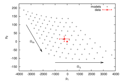
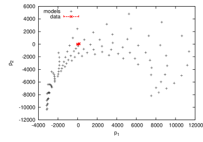
Figure 1: The first two features, i.e. the first two components of the feature vectors $\@vec{\tau}$, of an ensemble of Friedmann cosmologies with $h=0.7$, $w_{DE}=-1$, $\sigma_{8}=0.8$, and the matter density and dark energy density ranging in the intervals $0.1<\Omega_{m}<0.5$ and $0.5<\Omega_{\Lambda}<0.9$, respectively. Each black point is related to the corresponding $i$-th cosmological model by the mapping $\@vec{\tau}_{i}=\@vec{W}^{T}\@vec{t}_{i}$. The left panel refers to SNLS data alone and the right panel to WMAP-5yr data alone. The red points mark the feature space origin, i.e. the reference model $\bar{\@vec{t}}$, and the red points with error bars show the projection of the two data sets.

2 An optimised basis system for cosmological data sets

Table 1: Summary of the adopted main quantities.

Data set	$\@vec{d}\;\in\;\mathbb{R}^{n}$,	where   $n$ is the number of data points
Training vectors	$\@vec{t}_{i}\;\in\;\mathbb{R}^{n}$	with   $i=1,...,M$
Reference vector/model	$\bar{\@vec{t}}\;\in\;\mathbb{R}^{n}$	e.g.   $\bar{\@vec{t}}=\langle\@vec{t}\rangle$
Principal components	$\@vec{w}_{i}\;\in\;\mathbb{R}^{n}$	with   $i=1,...,n$
Feature vector	$\@vec{\tau}=\@vec{W}^{T}\@vec{t}\;\in\;\mathbb{R}^{n}$	where   $\@vec{W}=\left(\@vec{w}_{1},\@vec{w}_{2},...,\@vec{w_{n}}\right)$

This section presents an application of principal component analysis to cosmological data sets. In contrast with literature, we do not search for the principal components describing physical quantities within a specific cosmological model (e.g. the dark energy equation of state parameter $w$). Instead, we aim at the principal components which directly describe cosmological observables (e.g. luminosity distances, the CMB power spectrum, etc.). Their derivation does not involve any data set but it is only based on the predicted behaviour of cosmological models with different parameters or physical assumptions. The data set may (or not) enter in a second moment, where it can be analysed by means of the principal components.

The transformation identified with these principal components is defined such as to maximise the capability of discerning different cosmological models and to highlight the possible existence of unexpected features not foreseen when a specific model is adopted. We derive our approach having in mind the analysis of cosmological data sets, but its application is completely general.

2.1 Principal components derivation

We represent any data set with a vector $\@vec{d}\;\in\mathbb{R}^{n}$ whose dimension $n$ corresponds to the number of available data points, e.g. the number of observed supernovae luminosity distances $\@vec{d}=\left[D_{l}(z_{1}),D_{l}(z_{2}),...,D_{l}(z_{n})\right]$ or CMB power spectrum multipoles $\@vec{d}=\left[C(l_{1}),C(l_{2}),...,C(l_{n})\right]$. This allows one to consider the whole data set as a single point belonging to an $n-$dimensional space. This $n$-dimensional space, containing all of these possible $n$-vectors, makes it possible to address the problem directly through observable quantities regardless of their underling physics.

To probe the possible observables behaviour, we investigate this space by populating it with a set of $M$ vectors $\left\{\@vec{t}_{i}\;\in\;\mathbb{R}^{n}\;\mid\;i=1,...,M\right\}$ modelling the nature of the observed quantity, e.g. luminosity distances or CMB power spectrum multipoles, and distributed such as to include the data set. Since the ensemble of these models initialises our method, we refer to it as the training set in full analogy to other applications of the same and of similar techniques. In fact, also in morphological or spectral classification the training set is an ensemble of vectors sampling the possible behaviours expected in the data. In the same way, we sample the possible behaviours of cosmological observables to obtain a basis system capable to distinguish the different underlying cosmologies. For convenience, we organise the training set in a matrix,

$$\@vec{T}=\left(\@vec{t}_{1},\@vec{t}_{2},...,\@vec{t_{M}}\right)\;\in\;\mathbb{R}^{n\times M}\;,$$ (1)

where the $\@vec{t}_{i}$ vectors have the same structure of the analysed data, which can be discrete and irregular as for example the redshift coverage of a given supernova survey. In principle, these models can be a set of arbitrary functions, and actually the choice is fully arbitrary, but it is convenient to consider models at least weakly resembling the data set. It is in fact pointless to sample the entire domain of behaviours when we at least know the main data properties. The choice of the training set only determines for which kind of models, or better behaviours of the observables, the derived principal components performance is optimal. This is the reason why we find convenient to use a set of theoretical models. This choice does not preclude the method flexibility as it will be demostrated.

Once the training set models are defined, their information content can be optimised via a linear transformation $W:\mathbb{R}^{n}\rightarrow\mathbb{R}^{n}$ mapping the training-set vectors into a space (hereafter feature space) where their projections,

$$\@vec{\tau}_{i}=\@vec{W}^{T}\@vec{t}_{i}\;\in\;\mathbb{R}^{n}\;\quad\mbox{with}\quad i=1,...M\;,$$ (2)

have the maximum separation in very few components. We call feature vectors any vector resulting from the projection expressed by Eq. (2) and features their components. The linear transformation, $\@vec{W}=\left(\@vec{w}_{1},\@vec{w}_{2},...,\@vec{w_{n}}\right)$, satisfying the desired properties, i.e. concentrating in very few features all information regarding the differences between the models accounted in the training set, is given by a set of $n$ orthonormal vectors $\left\{\@vec{w}_{i}\;\in\;\mathbb{R}^{n}\;\mid\;i=1,...,n\right\}$ known as principal components. The principal components are found by solving the following eigenvalue problem

$$\@vec{w}_{i}=\lambda_{i}\,\@vec{S}\@vec{w}_{i}\;,$$ (3)

and by sorting them in descending order $\lambda_{i}>\lambda_{i+1}$ to ensure the largest feature separation in the very first components. Here

$$\@vec{S}=\@vec{\Delta}\@vec{\Delta}^{T}\;\in\;\mathbb{R}^{n\times n}\;$$ (4)

with $\@vec{\Delta}=\left(\@vec{t}_{1}-\@vec{\bar{t}},\@vec{t}_{2}-\@vec{\bar{t}},...,\@vec{t}_{M}-\@vec{\bar{t}}\right)\;\in\mathbb{R}^{n\times M}$, is the so-called scatter matrix, which encodes the differences (or scatter) between each training vector $\@vec{t}_{i}$, i.e. a given model, and the reference vector $\@vec{\bar{t}}$ around which the scatter is maximised. The reference vector defines the origin of the feature space and is usually set as the mean of the training set $\bar{\@vec{t}}\equiv\langle\@vec{t}\rangle$, but a different $\@vec{\bar{t}}$ can be used instead, depending on the specific problem at hand. An interesting choice could be the best fit to a given cosmological model, so that all other models would be described as its perturbed states. We summarise in Tab. (1) all quantities involved in the principal component derivation.

The principal components derived with our approach provide an optimal basis system to describe a given cosmological observable for different cosmologies, as for example luminosity distances to SN Ia if the training set is constitued by luminosity distance models. Note that they constitute a full basis system for the training-set cosmologies only. However, they turn out to be very flexible and even able to reproduce behaviour not even present in the training-set models as shown in Sec. (4.2). In this work, we choose to base our training set on Friedmann $\Lambda$CDM cosmologies with different cosmological parameters, but of course other kinds of cosmological models can be used as well, such as e.g. cosmologies with dynamical dark energy, based on modified gravity theories, or even a mixture of them so that they can be optimally described at the same time.

2.2 Principal components as an optimisation problem

The derivation of the principal components can be interpreted as a constrained optimisation problem, where the subset of linear orthonormal transformation $\@vec{W}$ maximising the separation between different cosmologies is sought. This is achieved by maximising the functionals $L_{i}=\@vec{w}_{i}^{T}S\@vec{w}_{i}-\lambda_{i}^{-1}(\@vec{w}^{T}_{i}\@vec{w}_{i}-1)$ with respect to $\@vec{w}_{i}$, i.e. by looking for the solution of $\delta L_{i}/\delta{\@vec{w}^{T}}_{i}=0$. This leads to the eigenvalue problem expressed by Eq. (3) and consequently to the same principal components $\@vec{w}_{i}$. With this approach, the first principal component can be seen as an optimal matched filter which in this case operates directly on cosmological data sets (see, e.g. Seljak & Zaldarriaga, 1996; Maturi et al., 2005; Schäfer et al., 2006).

2.3 Speeding up computations

If the training vector number is smaller than their dimension, i.e. $M<n$, only the first $M$ principal components can be associated to non-vanishing eigenvalues. Therefore, only those components need to be derived. This is achieved by computing the $M$ eigenvectors $\@vec{w}^{\prime}\;\in\mathbb{R}^{M}$ of the matrix

$$\@vec{S}^{\prime}=\@vec{\Delta}^{T}\,\@vec{\Delta}\;\in\;\mathbb{R}^{M\times M}\;.$$ (5)

These are related to the first $M$ eigenvectors of the scatter matrix $\@vec{S}$ by $\@vec{w}_{i}=\@vec{\Delta}\@vec{w}_{i}^{\prime}$. The increase in computational speed is especially remarkable for large data sets, where $M\ll n$.

In addition to this gain in computational speed, all the relevant information is, in most cases, constrained by a very small number of independent components, $m<M$ (usually up to three for this kind of applications), allowing for an even stronger dimensionality reduction. In other words, a full data description is guaranteed by the subspace $\mathbb{R}^{m}$ sampled by the training set.

2.4 Combining different data sets

The approach described above represents a straightforward way to combine different observables for a joint data analysis. For example, if we want to combine the luminosity distances to SN Ia, the CMB angular power spectrum and the cosmic shear correlation function, we just need to organise the data vector in the form

$$\@vec{d}=\left[D_{l}(z_{1})\,...\,D_{l}(z_{n_{sn}}),\,C_{l_{1}}\,...\,C_{l_{n_{cmb}}},\,\xi(\theta_{1})\,...\,\xi(\theta_{n_{\xi}})\right]\;,$$ (6)

whose dimension is given by the sum of all data sets sizes $n=n_{sn}+n_{cmb}+n_{\xi}$. In order to work with non-dimensional quantities which reflect the signal-to-noise ratios, the different observables have to be re-normalised with respect to their variance. Of course the training set vectors format must be consistent with Eq. (6).

Figure 2: Example showing the stability of the principal components against the number of models used in the training-set. We show only the first 4 principal components derived for the luminosity distance sampled at the redshifts covered by the SuperNova Legacy Survey. The training-set was produced by sampling the parameter space in the range $0.1<\Omega_{m}<0.5$ and $0.5<\Omega_{\Lambda}<0.9$, 100 (left panel) and 5 times (right panel), respectively, and using as a reference cosmology the training-set average.

3 A new cosmological parameterisation

Since the features $\@vec{\tau}$ discussed in Sec. (2) retain all significant cosmological information, they can be used to parameterise cosmologies. In contrast with the ‘standard’ cosmological parameters, they aim to describe observable quantities instead of physical properties. To give a visual impression of how cosmologies are represented in the feature space, we show two simple examples in Fig. 1, for luminosity distances only (left panel) and CMB power spectra only (right panel). Here, we plot the first two components of the feature vectors resulting from the projection of an ensemble of non-flat $\Lambda$CDM models. Each point represents a $\Lambda$CDM cosmology with specific cosmological parameters. The principal components underlying this projection are based on a training set where only the matter and dark-energy densities are varied independently in the range $0.1<\Omega_{m}<0.5$ and $0.5<\Omega_{\Lambda}<0.9$, respectively. The Hubble constant in units of $100{\;\rm km/s/Mpc}$, the equation of state parameter of dark-energy and the matter fluctuations power spectrum normalisation were fixed to $h=0.7$, $w=-1$, $\sigma_{8}=0.8$, respectively. Note that, in the case of CMB data, the $\Omega_{m}-\Omega_{\Lambda}$ feature space plane is curved such that at least three features would be necessary for a satisfactory description of the most extreme cosmologies considered. This is because of the rich complexity of the data set. To cope with this, a non linear mapping could be used to ‘follow the distortion’ of the models hyper-plane in the feature space, but this would add unnecessary complications since the use of a larger number of features is not a limitation. In any case the actual CMB physical models have a large number of parameters with large mutual degeneracies (for instance the optical depth, the baryon fraction, the inflation spectral index, etc.), therefore the more complex models usually adopted are not necessarily described by a linearly growing number of features compensating the increase of necessary features.

With this formalism, the principal components can be considered as cosmological eigen-modes (eigen-cosmologies) where observations would “excite” (i.e. make visible) a given number of modes according to their accuracy.

3.1 The advantages

The use of these orthonormal functions to define a parameter set characterising observable behaviour instead of underlying physical quantities has several advantages. In fact:

• the features are fully independent by definition and therefore avoid any redundancy and degeneracy in the observable description, in contrast with physical parameterisations;

• they retain all available information because they are derived from the principal components;

• their number is minimal as allowed by the data accuracy;

• they provide the best discriminatory power for the family of cosmologies adopted in the training-set;

• they can be related to any physical model via the mapping $\@vec{\tau}_{i}=\@vec{W}^{T}\@vec{t}_{i}$ itself;

• the features allow one to quantify the overall difference between two cosmologies in terms of a simple metric separation

  $$s=\frac{\left|\@vec{\tau}_{1}-\@vec{\tau}_{2}\right|}{\left|\@vec{\tau}_{\sigma}\right|}\;,$$ (7)

  where $\@vec{\tau}_{1}$ and $\@vec{\tau}_{2}$ are the two cosmologies features vectors and $\@vec{\tau}_{\sigma}$ is the data uncertainty projection in the feature space.

These properties apply also to cosmologies which are not explicitly included in the training set; however, in this case not all model behaviours are ensured to be captured. In other words, if nature or the cosmological model we are investigating differs from the one adopted in the principal component definition, we could still use them, even if in suboptimal conditions. In any case, it is possible to cope with this by making the training set less specialised. If we are for example studying cosmologies based on different physical frameworks such as General Relativity, TeVeS or $f(R)$ theories or simply different dark-energy models, we could include all of them in the training set so that the resulting features can optimally describe all of them at the same time. Given that, it follows how the features $\@vec{\tau}$ can be used as a common parameterisation to describe and compare cosmologies even if based on different physical frameworks. Again, this is possible because this approach parameterises observables only and not their very diverse background physics. In this paper we only consider non-flat $\Lambda$CDM cosmologies for sake of simplicity.

3.2 Studying different modellisations degeneracies

The proposed parameterisation, thanks to the properties discussed in Sec. (3.1), provides a useful tool to study degeneracies in the same or, more interestingly, in different modellisations and physical frameworks. In fact, fully degenerate models show the same observational properties and consequently have the same features $\@vec{\tau}$. Of course, when considering observational data, degeneracies are not associated to a feature space point but to the hyper-volume defined by the data errors projection. In fact also data errors have to be projected into the feature space to define the region compatible with the data as shown in Fig. (1). All information regarding how similar, i.e. degenerate, two models are is quantified by the metric distance given in Eq. (7) which is in fact normalised with respect to the data accuracy. In fact, all models whose separation is smaller than the hyper-volume radius allowed by data are degenerate.

In comparison with Markov-Chain Monte Carlo methods (see for example Lewis & Bridle, 2002), this approach is not an iterative method and is computationally cheap since a small number of models have to be computed. In fact, the parameter space can be sampled on a very coarse grid and, if necessary, according to the parameters conditional distribution in analogy with Gibbs sampling. In a follow up paper we will discuss a detailed study of this parameterisation and of its application in degeneracy studies.

4 Hubble expansion rate from supernovae data

Supernova luminosity distances are a very powerful probe to investigate cosmology. In particular, they can be used to directly measure the expansion history of the universe, $H(a)$, avoiding any reference to Friedmann models. In fact, if we assume a topologically simply connected, homogeneous and isotropic universe, the luminosity distance can be expressed as

$$D_{L}(a)=\frac{c}{H_{0}\;a}\int_{a}^{1}\frac{\mathrm{d}x}{x^{2}}e(x)\;,$$ (8)

where the expansion function is expressed as $H(a)=H_{0}E(a)$, with $H_{0}$ being the Hubble expansion constant and $e(a)\equiv E^{-1}(a)$ the inverse expansion rate. For the sake of simplicity, we drop the $c/H_{0}$ factor in the following discussion.

The Hubble expansion function can be directly derived from a luminosity distance data set, as detailed in MB08. In fact, the derivative of Eq. (8) with respect to the scale factor, $a$, can be brought into the form of a Volterra integral equation of the second kind,

$$e(a)=-a^{3}D^{\prime}_{L}(a)+a\int_{1}^{a}\frac{\mathrm{d}x}{x^{2}}e(x)\;,$$ (9)

whose solution, $e(a)$, can be expressed in terms of a Neumann series (see for e.g. Arfken & Weber, 1995),

$$e(a)=\sum_{i=0}^{\infty}a^{i}f_{i}(a)\;,$$ (10)

where a possible choice for the expansion terms $f_{i}$ is

$$f_{0}(a)=-a^{3}D^{\prime}_{L}(a)\;,\quad f_{i}(a)=\int_{1}^{a}\frac{\mathrm{d}x}{x^{2}}f_{i-1}\;.$$ (11)

Here it is necessary to smooth the observational data, $D_{L}(a)$, to avoid possible issues with the intrinsic data scatter when estimating the derivative $D^{\prime}_{L}(a)$. A convenient way to do it is to expand the luminosity distance data into a set of orthonormal functions

$$D_{L}(a)=\sum_{j=0}^{M}c_{j}p_{j}(a)\;,$$ (12)

where the coefficients $c_{j}$ are determined from data fitting. This approach has the advantage of avoiding all assumptions regarding the energy content of the universe, thus making the reconstruction nearly model-independent.

The choice of the adopted basis, $\{p_{j}\}$ in Eq. (12), is arbitrary. For illustrative reasons, MB08 adopted the linearly independent set $u_{j}(a)=a^{j/2-1}$ ortho-normalised with the Gram-Schmidt process. However, the basis $\{p_{j}\}$ can be defined such as to minimise the number of necessary modes and to have them ordered according to their information content. A good choice fulfilling these criteria is represented by the principal components defined in Sec. (2) which can be optimised for a specific cosmology or for a set of cosmological models based on different physical assumptions. This basis optimisation enhances the MB08 method performances without precluding its flexibility. In fact, also behaviours not described by the models adopted in the basis definition can be reproduced, as it will be shown in Sec. (4.2).

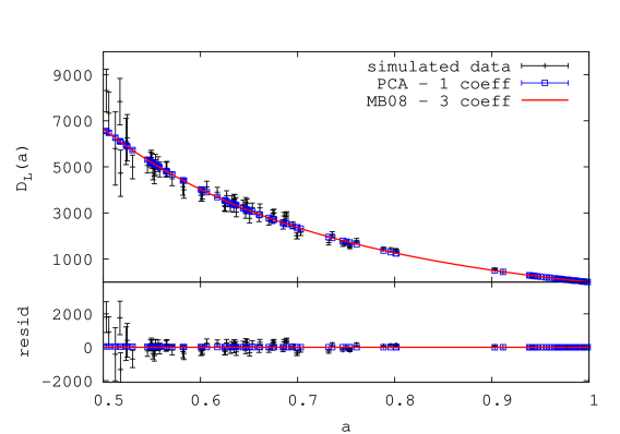
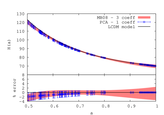
Figure 3: Fit of our supernovae luminosity distances mock catalogue resembling the SNLS data set (left panel) and the recovered expansion rate obtained (right panel). We compare the results obtained by using the original MB08 recipe (shaded area) and by using our principal components as basis set (blue squares). The increased accuracy is especially evident at lower redshifts, where the method improvement takes fully advantage of the smaller measurement errors.

4.1 Principal components stability

The stability of the principal components with respect to the number of models used in the training set has been tested. We show in Fig. 2 the first four principal components derived for a luminosity-distance data vector with the same redshift sampling of the SuperNova Legacy Survey (Astier et al., 2006). The training set is based on non-flat $\Lambda$CDM models with $h=0.7$, $w=-1$ and the matter and dark-energy density parameters sampling the ranges $0.1<\Omega_{m}<0.5$ and $0.5<\Omega_{\Lambda}<0.9$, respectively; as a reference cosmology, the average of the training set has been used. The ($\Omega_{m},\Omega_{\Lambda}$) space was regularly sampled by the training set $10,000$ times to produce the left panel and only $25$ times in the right panel. Clearly, the principal components are very stable against the training-set size and only depend on the range spanned by the cosmological parameters of the training set.

As discussed in Sec. (2), the information content of each principal component is quantified by the corresponding eigenvalue, which in this case are $\lambda_{1}=1$, $\lambda_{2}=2.0\,10^{-4}$, $\lambda_{3}=1.4\,10^{-7}$ and $\lambda_{4}=1.2\,10^{-10}$. Hence, all information and discriminatory power is concentrated in the very first components allowing for a strong dimensionality reduction, from $n=117$ (i.e. the number of supernovae in the data set) to 1 or 2 dimensions for this specific case. If the number of parameters sampled in the training-set construction is increased, or if the intervals over which they are sampled are larger, the power is distributed towards higher orders, but is still fairly concentrated in very few components.

4.2 Application to synthetic data: highlighting unexpected features

We apply the MB08 method combined with the principal components described in Sec. (2) on a synthetic data sample drawn from a $\Lambda$CDM model with $\Omega_{M}=0.3$, $\Omega_{\Lambda}=0.7$ and $h=0.7$, and resembling the SNLS properties (Astier et al., 2006). The training set for the principal components definition is the same tested in Sec. (4.1). We show in Fig. 3 the resulting fit to the data (left panel) and the subsequently estimated expansion rate (right panel) as compared with the original MB08 recipe (shaded area). The resulting error bars are smaller when the principal components are used since the adopted basis is optimised for $\Lambda$CDM cosmologies and less parameters have to be fitted: one coefficient, rather than three. The increased accuracy is particularly evident at lower redshifts, where the method improvement takes fully advantage of the smaller measurement errors.

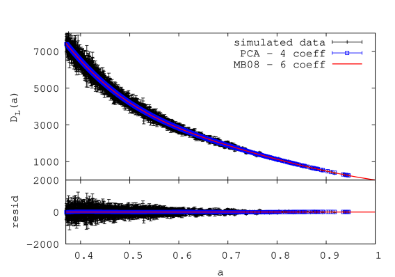
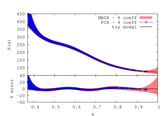
Figure 4: Same as in Fig. 3, but for a SNAP like mock catalogue based on a toy-model simulation with a sharp transition in the expansion rate. Even if the training-set was defined on Friedmann models without such a feature, the reconstruction was capable to highlight it.

As a second test case, we now consider a more challenging data set in order to test the method’s capability of capturing behaviours not explicitly described by the training-set models. In this example, we use the same training set of the previous case but we analyse luminosity distances resulting from a toy-model cosmology with a sudden transition in the expansion rate (see MB08 for details). In this case, the sample observational characteristics are modelled after the proposed satellite SNAP (Aldering, 2005). A $\chi^{2}$-analysis shows that this simulated data are compatible with a standard Friedmann $\Lambda$CDM cosmology. This is of course a misleading result since the background cosmology has a completely different nature and the sudden transition in $H(a)$ is not highlighted. This demonstrates how a standard $\chi^{2}$-approach is not always capable of revealing the unexpected features hidden in the data set and how the result is bound to the theoretical prejudice. In contrast, with the proposed method this expansion rate transition is observed even if the training set does not contain any model with such a feature. The reconstructed expansion rate for this example is shown in Fig. 4 (blue error bars) together with the one obtained with the method as originally proposed by MB08 (shaded area). The accuracy improvement with respect to the original MB08 method may not appear striking, but we have to consider that this is a very extreme case where not even the best-fit Friedmann model is covered by the training set. This example just demonstrates the method’s capability of capturing unexpected features even if optimised only for a specific set of cosmologies.

4.3 Results on the SNLS data set

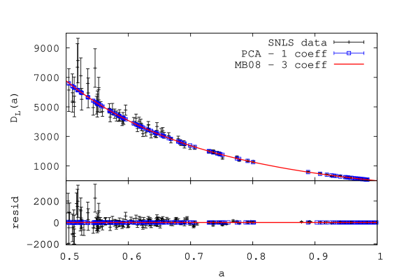
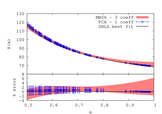
Figure 5: Same as in Fig. 3 but for the real SNLS data set. The reconstruction accuracy is largely improved and is fully compatible with the best-fit $\Lambda$CDM model.

The SuperNova Legacy Survey data set consists of 118 supernovae in the redshift range $0.015<z<1.01$, 71 observed with the Canada-France-Hawaii Telescope and 44 taken from the literature (Astier et al., 2006). We analysed this sample with the same procedure applied to the $\Lambda$CDM simulation discussed in Sec. (4.2). The result shown in Fig. 5 is fully compatible with the best $\Lambda$CDM model fit (Astier et al., 2006). The accuracy is largely improved with respect to the original MB08 reconstruction, giving the hope that future supernova samples may be able to reveal the dark-energy nature.

5 Conclusions

We defined an optimal basis system based on principal components to decompose cosmological observables. The principal components are defined starting not from the data but from an ensemble of given models. The basis system can be optimised for a specific cosmological model or for an ensemble of models even if based on different physical hypotheses. We suggest two main applications: (1) to define a cosmological parameterisation applicable to any model independently of the physical background and (2) to optimise the MB08 method for a direct estimate of the expansion rate from luminosity distance data.

On one hand, the cosmological parameterisation is based on the coefficients, i.e. the features, resulting from the observables projection on the discussed basis system. The features are fully independent, avoiding the degeneracies and redundancies of physical parameters, and their number is minimal with respect to the data accuracy. Since they quantify observable properties, they can be used as a common parameterisation to describe cosmologies independently of their background physics. However, they can be uniquely related to physical parameters once a model is specified. In addition, this parameterisation allows one to quantify the differences between different cosmologies in terms of a simple metric separation.

On the other hand, the method proposed by MB08, which directly estimates the expansion rate from supernova data, requires to expand luminosity distances into a set of arbitrary orthonormal functions. The use of the basis system derived in this work largely reduces the resulting uncertainties and, even if the method is only optimised for a single or for an ensemble of cosmological models, it is still capable to detect unforeseen features not included in the algorithm setup as demonstrated.