Numerical Solutions of the Isotropic 3-Wave Kinetic Equation

Abstract

We show that the isotropic 3-wave kinetic equation is equivalent to the mean field rate equations for an aggregation-fragmentation problem with an unusual fragmentation mechanism. This analogy is used to write the theory of 3-wave turbulence almost entirely in terms of a single scaling parameter. A new numerical method for solving the kinetic equation over a large range of frequencies is developed by extending Lee’s method for solving aggregation equations. The new algorithm is validated against some analytic calculations of the Kolmogorov-Zakharov constant for some families of model interaction coefficients. The algorithm is then applied to study some wave turbulence problems in which the finiteness of the dissipation scale is an essential feature. Firstly, it is shown that for finite capacity cascades, the dissipation of energy becomes independent of the cut-off frequency as this cut-off is taken to infinity. This is an explicit indication of the presence of a dissipative anomaly. Secondly, a preliminary numerical study is presented of the so-called bottleneck effect in a wave turbulence context. It is found that the structure of the bottleneck depends non-trivially on the interaction coefficient. Finally some results are presented on the complementary phenomenon of thermalisation in closed wave systems which demonstrates explicitly for the first time the existence of so-called mixed solutions of the kinetic equation which exhibit aspects of both Kolmogorov-Zakharov and equilibrium equipartition spectra.

I Introduction

The 3-wave kinetic equation is the analogue of the Boltzmann equation for an ensemble of nonlinear dispersive waves interacting weakly via a quadratic nonlinearity in the wave equation. Such wave systems are often conveniently modeled using Hamiltonian equations for the complex wave amplitudes, $a_{{\mathbf{k}}}$ supplemented with additional terms modeling forcing, $f_{{\mathbf{k}}}$, and dissipation, $\Gamma_{{\mathbf{k}}}$:

$$\frac{\partial a_{{\mathbf{k}}}}{\partial t}=i\frac{\delta H}{\delta\bar{a}_{{\mathbf{k}}}}+f_{{\mathbf{k}}}-\Gamma_{{\mathbf{k}}}a_{{\mathbf{k}}}.$$ (1)

The Hamiltonian, $H$, contains quadratic and cubic terms in the wave amplitudes, $a_{{\mathbf{k}}}$:

$$H=\int\omega_{\mathbf{k}}a_{{\mathbf{k}}}\bar{a}_{{\mathbf{k}}}d{\mathbf{k}}+\int u({\mathbf{k}})d{\mathbf{k}},$$ (2)

where

$$u({\mathbf{k}}_{1})\!\!\!=\!\!\!\int L_{{\mathbf{k}}_{1}{\mathbf{k}}_{2}{\mathbf{k}}_{3}}\left(a_{{\mathbf{k}}_{1}}a_{{\mathbf{k}}_{2}}\bar{a}_{{\mathbf{k}}_{3}}+\bar{a}_{{\mathbf{k}}_{1}}\bar{a}_{{\mathbf{k}}_{2}}a_{{\mathbf{k}}_{3}}\right)\delta({\mathbf{k}}_{1}-{\mathbf{k}}_{2}-{\mathbf{k}}_{3})\,d{\mathbf{k}}_{2}d{\mathbf{k}}_{3}.$$ (3)

The theory of weak wave turbulence Zakharov et al. (1992); Newell et al. (2001) studies the statistical evolution of the solutions of Eq. (1) in the situation where the nonlinear term can be treated as a perturbation. Within the framework of weak wave turbulence, the 3-wave kinetic equation is derived as a consistent asymptotic closure of the cumulant hierarchy generated by Eq. (1). It describes the time evolution of the spectral wave-action density, $n_{{\mathbf{k}}}$, which, for statistically homogeneous wave fields, is obtained from the two-point correlation function of the wave amplitudes:

$$\langle a_{{\mathbf{k}}_{1}}\bar{a}_{{\mathbf{k}}_{2}}\rangle=n_{{\mathbf{k}}_{1}}\,\delta({\mathbf{k}}_{1}-{\mathbf{k}}_{2}).$$ (4)

It takes the form

$$\frac{\partial n_{\mathbf{{\mathbf{k}}}_{1}}}{\partial t}=S[n_{\mathbf{k}}]+F[n_{\mathbf{k}}]-D[n_{\mathbf{k}}].$$ (5)

$F[n_{\mathbf{k}}]$, which is absent for decay problems, represents the wave forcing. $D[n_{\mathbf{k}}]$ represents dissipation and is typically only present at high wave-vectors. $S[n_{\mathbf{k}}]$, referred to as the collision integral, describes the conservative transfer of energy between wave modes due to resonant interactions and is the term responsible for the energy cascade. We shall study its explicit form in Sec. II.

It is convenient, and physically relevant, to consider isotropic scale invariant systems. This means that both the dispersion relation and the nonlinear interaction coefficient are homogeneous functions of their arguments without any preferred direction. We denote their degrees of homogeneity by $\alpha$ and $\beta$ respectively:

$$\omega_{a\,k} = a^{\alpha}\,\omega_{{\mathbf{k}}}$$ (6)

$$L_{a{\mathbf{k}}_{1}a{\mathbf{k}}_{2}a{\mathbf{k}}_{3}} = a^{\beta}\,L_{{\mathbf{k}}_{1}{\mathbf{k}}_{2}{\mathbf{k}}_{3}}.$$

For convenience, we shall take the dispersion relation to be a simple power law:

$$\omega{k}=\omega{k}=c\,\omega^{\alpha}.$$ (7)

A huge amount is known about the stationary solutions of Eq. (5) in the turbulent regime where the forcing and dissipation scales are asymptotically separated from each other in scale. In addition to the thermodynamic equilibrium solution, there exists an exact stationary non-equilibrium solution, known as the Kolmogorov-Zakharov spectrum, which carries a constant flux of energy through scales. This energy cascade solution is the analogue of the (phenomenological) Kolmogorov $k^{-5/3}$ spectrum of hydrodynamic turbulence. The fact that the energy cascade spectrum can be derived analytically is one of the principle reasons for theoretical interest in weak wave turbulence.

Rather less is known about the solutions of Eq. (5) beyond the characterisation of the stationary state in the limit where the forcing and dissipation scales tend to zero and infinity respectively. In particular, knowledge about the dynamical evolution of the solutions is restricted to a subset of systems for which a self-similar solution can be constructed using energy conservation arguments which in any case, leave the scaling function undetermined. Similarly relatively little is known about how the system matches itself to the source and sink in the case of finite forcing and dissipation scales which break the scale invariance necessary to obtain the K-Z solution. It is in this context that the present work fits.

This article contains two main ideas. The first is that in the case of isotropic systems, the 3-wave kinetic equation is equivalent to the rate equations for an aggregation-fragmentation problem with a rather unusual fragmentation process. This is useful for several reasons. Firstly, there is a large body of knowledge about rate equations for aggregation-fragmentation problems which might provide useful insights. Secondly, this description is very compact with almost all properties of the solution being determined by a single scaling parameter. Thirdly, and this forms the basis for the second main idea of the article, this description forms the basis for a new numerical procedure for solving the 3-wave kinetic equation which can resolve a very large range of scales compared to a direct numerical integration. This numerical procedure can then be used to investigate aspects of 3-wave turbulence which are less amenable to analytic understanding.

The layout of the article is as follows. We first explain in Sec. IIthe analogy between 3-wave turbulence and aggregation-fragmentation equations, with the technical details relegated to an appendix. One of the principle insights provided by this analogy is that most of the scaling properties of the system are determined by a single parameter, $\lambda=\frac{2\beta-\alpha}{\alpha}$. In Sec. III we devote some time to explaining how the standard results of weak wave turbulence are expressed in terms of $\lambda$. In Sec. IV we consider truncating the system at some finite frequency and discuss open and closed truncations, two distinct natural choices of truncation. In Sec. V the results of Sec. II and Sec. IV are used to develop a new numerical procedure which allows the stable integration of the 3-wave kinetic equation over many decades of frequencies. Some technical details of the method are postponed to a second appendix. The remainder of the article is then devoted to presenting some preliminary studies which are intended to demonstrate the usefulness of this algorithm. In Sec. VII we study the numerical signature of the dissipative anomaly in finite capacity cascades. In Sec. VIII we demonstrate the non-trivial structure of the bottleneck effect in the 3-wave kinetic equation with an open truncation and in Sec. IX we study the thermalisation phenomenon which occurs when the equation is subjected to a closed truncation. The article closes with some conclusions and speculations about future directions of research.

II Formulation of the Isotropic 3-Wave Kinetic Equation as an Aggregation–Fragmentation Problem

The collision integral is usually written in the form

$$S[n_{\mathbf{k}}]=\int_{{\mathbf{R}}^{2d}}\left(R_{{\mathbf{k}}_{1}{\mathbf{k}}_{2}{\mathbf{k}}_{3}}-R_{{\mathbf{k}}_{2}{\mathbf{k}}_{3}{\mathbf{k}}_{1}}-R_{{\mathbf{k}}_{3}{\mathbf{k}}_{1}{\mathbf{k}}_{2}}\right)\,d{\mathbf{k}}_{2}d{\mathbf{k}}_{2}$$ (8)

where

$$R_{{\mathbf{k}}_{1}{\mathbf{k}}_{2}{\mathbf{k}}_{3}} = 4\pi\,L_{{\mathbf{k}}_{1}{\mathbf{k}}_{2}{\mathbf{k}}_{3}}^{2}(n_{{\mathbf{k}}_{2}}n_{{\mathbf{k}}_{3}}-n_{{\mathbf{k}}_{1}}n_{{\mathbf{k}}_{3}}-n_{{\mathbf{k}}_{1}}n_{{\mathbf{k}}_{2}})$$

$$\hskip 14.22636pt\delta(\omega_{{\mathbf{k}}_{1}}-\omega_{{\mathbf{k}}_{2}}-\omega_{{\mathbf{k}}_{3}})\,\delta({\mathbf{k}}_{1}-{\mathbf{k}}_{2}-{\mathbf{k}}_{3})$$

The total wave-action, $N$, and total quadratic energy, $E$, in the system are

$$N = \int_{{\mathbf{R}}^{d}}n_{\mathbf{k}_{1}}\,d{\mathbf{k}}_{1}$$ (9)

$$E = \int_{{\mathbf{R}}^{d}}\omega_{{\mathbf{k}}_{1}}\,n_{\mathbf{k}_{1}}\,d{\mathbf{k}}_{1}$$ (10)

respectively. $E$ is conserved by Eq. (5) in the absence of forcing and dissipation. For isotropic systems it is convenient to work with the angle-averaged frequency spectrum, $N_{\omega}$ instead of the basic ${\mathbf{k}}$-space spectrum, $n_{\mathbf{k}}$. $N_{\omega}$ is defined such that $\int_{\omega_{1}}^{\omega_{2}}N_{\omega}\,d\omega$ is the total wave action in the frequency band $[\omega_{1},\omega_{2}]$. It is shown in the appendix that, for isotropic systems, Eq. (5) is equivalent to

$$\frac{\partial N_{\omega_{1}}}{\partial t}=S_{1}[N_{\omega}]+S_{2}[N_{\omega}]+S_{3}[N_{\omega}]+F[N_{\omega}]-D[N_{\omega}]$$ (11)

where

$$S_{1}[N_{\omega}]\!\!\! = \!\!\!\!\!\int\!\!K_{1}(\omega_{2},\omega_{3})\,N_{\omega_{2}}N_{\omega_{3}}\delta(\omega_{1}\!-\!\omega_{2}\!-\!\omega_{3})\,d\omega_{23}$$

$$- \!\!\!\!\!\int\!\!K_{1}(\omega_{3},\omega_{1})\,N_{\omega_{1}}N_{\omega_{3}}\delta(\omega_{2}\!-\!\omega_{3}\!-\!\omega_{1})\,d\omega_{23}$$

$$- \!\!\!\!\!\int\!\!K_{1}(\omega_{1},\omega_{2})\,N_{\omega_{1}}N_{\omega_{2}}\delta(\omega_{3}\!-\!\omega_{1}\!-\!\omega_{2})\,d\omega_{23},$$

$$S_{2}[N_{\omega}]=\!\!\! - \!\!\!\!\!\int\!\!K_{2}(\omega_{2},\omega_{3})\,N_{\omega_{1}}N_{\omega_{2}}\delta(\omega_{1}\!-\!\omega_{2}\!-\!\omega_{3})\,d\omega_{23}$$

$$+ \!\!\!\!\!\int\!\!K_{2}(\omega_{3},\omega_{1})\,N_{\omega_{2}}N_{\omega_{3}}\delta(\omega_{2}\!-\!\omega_{3}\!-\!\omega_{1})\,d\omega_{23}$$

$$+ \!\!\!\!\!\int\!\!K_{2}(\omega_{1},\omega_{2})\,N_{\omega_{1}}N_{\omega_{3}}\delta(\omega_{3}\!-\!\omega_{1}\!-\!\omega_{2})\,d\omega_{23}$$

and

$$S_{3}[N_{\omega}]=\!\!\! - \!\!\!\!\!\int\!\!K_{3}(\omega_{2},\omega_{3})\,N_{\omega_{1}}N_{\omega_{3}}\delta(\omega_{1}\!-\!\omega_{2}\!-\!\omega_{3})\,d\omega_{23}$$

$$+ \!\!\!\!\!\int\!\!K_{3}(\omega_{3},\omega_{1})\,N_{\omega_{1}}N_{\omega_{2}}\delta(\omega_{2}\!-\!\omega_{3}\!-\!\omega_{1})\,d\omega_{23}$$

$$+ \!\!\!\!\!\int\!\!K_{3}(\omega_{1},\omega_{2})\,N_{\omega_{2}}N_{\omega_{3}}\delta(\omega_{3}\!-\!\omega_{1}\!-\!\omega_{2})\,d\omega_{23}.$$

$F[N_{\omega}]$ and $D[N_{\omega}]$ are forcing and dissipation terms whose exact forms depend on the problem under consideration. In these formulae, as shown in the appendix, $K_{1}(\omega_{i},\omega_{j})$, $K_{2}(\omega_{i},\omega_{j})$ and $K_{3}(\omega_{i},\omega_{j})$ are homogeneous functions which an be constructed from the original interaction coefficient, $L_{{\mathbf{k}}_{1}{\mathbf{k}}_{2}{\mathbf{k}}_{3}}$. They all have degree of homogeneity

$$\lambda=\frac{2\beta-\alpha}{\alpha}.$$ (15)

We have therefore already obtained a nontrivial result which seems to have gone unnoticed before: all scaling properties of Eq. (5), which contains 3 scaling parameters, $\alpha$,$\beta$ and $d$, seem to depend on a single scaling parameter, $\lambda$ given by Eq. (15). In fact, this is not completely true. Owing to the fact that $K_{1}(\omega_{i},\omega_{j})$, $K_{2}(\omega_{i},\omega_{j})$ and $K_{3}(\omega_{i},\omega_{j})$ are not identical functions (even though they have the same degree of homogeneity), some memory of $\alpha$,$\beta$ and $d$ is retained in their internal structure - see Eq. (104) - which can sometimes be important. The details of what can and cannot be expressed solely in terms of the new parameter, $\lambda$, will be addressed in Sec. III.

(A) : $S_{1}[N_{\omega}]$:

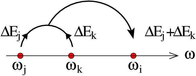
(B) : $S_{2}[N_{\omega}]$:

(C) : $S_{3}[N_{\omega}]$:

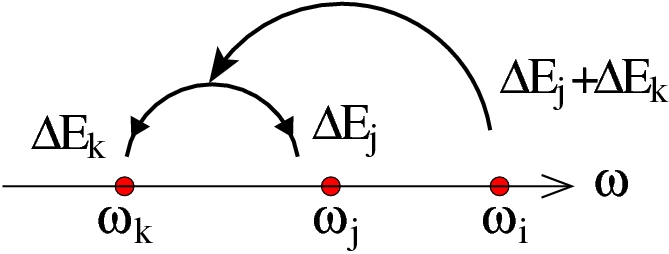
Figure 1: Graphical representations of the dynamics encoded by Eq. (II), Eq. (II) and Eq. (II).

Let us first investigate the physical meaning of Eq. (II) – Eq. (II). Firstly, it is easily shown that each of the three collision integrals, $S_{1}[N_{\omega}]$, $S_{2}[N_{\omega}]$ and $S_{3}[N_{\omega}]$, individually conserve the total energy.

Let us first consider Eq. (II) in isolation. The resulting kinetic equation

$$\frac{\partial N_{\omega_{1}}}{\partial t}=S_{1}[N_{\omega}],$$ (16)

is actually the Smoluchowski kinetic equation Leyvraz (2003) which describes the mean-field dynamics of cluster–cluster aggregation although it has been written in a somewhat non-standard form Connaughton et al. (2004, 2009). We can therefore make an analogy between wave turbulence and cluster–cluster aggregation. In this analogy, wave frequency, $\omega$, is analogous to cluster mass, $m$, spectral wave-action density, $N_{\omega}$, is analogous to density of clusters having mass $m$, $N_{m}$ and the wave interaction coefficient, $K_{1}(\omega_{1},\omega_{2})$ is analogous to the coagulation kernel, $K(m_{1},m_{2})$.

The physical meaning of the collision integral is easy to understand in the aggregation context. In coagulation, pairs of clusters having masses $m_{j}$ and $m_{k}$ aggregate to produce a single cluster having mass $m_{i}=m_{j}+m_{k}$. The rate at which this process occurs, as for any chemical rate equation, is proportional to the aggregation kernel, $K(m_{j},m_{k})$, and to the densities of clusters having masses, $m_{j}$ and $m_{k}$. This can be thought of an exchange of mass within the mass triad, $(m_{i},m_{j},m_{k})$. The mass contained in clusters of mass $m_{j}$ decreases at a rate $m_{j}K(m_{j},m_{k})N_{m_{j}}N_{m_{k}}$, the mass contained in clusters of mass $m_{k}$ decreases at a rate $m_{k}K(m_{j},m_{k})N_{m_{j}}N_{m_{k}}$ while the mass contained in clusters of mass $m_{i}$ increases at a rate $(m_{j}+m_{k})\,K(m_{j},m_{k})\,N_{m_{j}}\,N_{m_{k}}$. Clearly mass is conserved overall. The collision integral therefore simply calculates the net rate of change of the density of clusters of a given mass by summing the contributions of this process over all mass triads. The signs of the terms composing the collision integral now make perfect sense: the first (positive) term accounts for the rate of increase of clusters of mass $m_{1}$ due to the aggregation of pairs of smaller clusters having masses $m_{2}$ and $m_{3}$ which satisfy $m_{2}+m_{3}=m_{1}$. The second and third (negative) terms account for the rate of decrease of clusters of mass $m_{1}$ which occurs when such clusters meet any other cluster having mass $m_{2}$ or $m_{3}$ and aggregate to produce a heavier cluster having mass $m_{1}+m_{2}$ of $m_{1}+m_{3}$. Of course, these two negative terms are usually combined into a single term since they differ only by the labeling of dummy variables. Nevertheless, for reasons which will become apparent in Sec. III we choose to keep the rather verbose form of Eq. (II).

Taking this over to the wave analogy, we see that the first term on the RHS of Eq. (5) describes a transfer of energy in resonant triads, $(\omega_{i},\omega_{j},\omega_{k})$. That is to say, triads for which $\omega_{i}=\omega_{j}+\omega_{k}$. The energy contained in waves of frequency $\omega_{j}$ decreases at a rate $\omega_{j}K_{1}(\omega_{j},\omega_{k})N_{\omega_{j}}N_{\omega_{k}}$, the energy contained in waves of frequency $\omega_{k}$ decreases at a rate $\omega_{k}K_{1}(\omega_{j},\omega_{k})N_{\omega_{j}}N_{\omega_{k}}$ while the energy contained in waves of frequency $\omega_{i}$ increases at a rate $(\omega_{j}+\omega_{k})\,K_{1}(\omega_{j},\omega_{k})\,N_{\omega_{j}}\,N_{\omega_{k}}$. The rates of energy transfer for each mode in the triad $(\omega_{i},\omega_{j},\omega_{k})$ can thus be summarised as

$$\omega_{j} : \Delta E_{j}=-\omega_{j}K_{1}(w_{j},w_{k})N_{\omega_{j}}N_{\omega_{k}}$$

$$\omega_{k} : \Delta E_{k}=-\omega_{k}K_{1}(w_{j},w_{k})N_{\omega_{j}}N_{\omega_{k}}$$ (17)

$$\omega_{i} : \Delta E_{i}=+(\Delta E_{j}+\Delta E_{k}).$$

This process is illustrated graphically in Fig. 1(A). The collision integral then calculates the net rate of change of the energy of the waves of each frequency by summing the contributions of this process over all resonant triads. It is clear from this discussion that energy can only be transferred from lower frequencies to higher frequencies by the collision integral $S_{1}[N_{\omega}]$. As we shall see below, the reverse is the case for the integrals $S_{2}[N_{\omega}]$ and $S_{3}[N_{\omega}]$. $S_{1}[N_{\omega}]$ is therefore the driver of the direct cascade in wave turbulence.

If we have laboured the point a little on the interpretation of $S_{1}[N_{\omega}]$ and the analogy with aggregation, it is because the corresponding interpretation of $S_{2}[N_{\omega}]$ and $S_{3}[N_{\omega}]$ is less obvious. Indeed, the dynamics encoded by these integrals illustrates clearly why wave resonances are different from particles. We first notice that the sign structure of $S_{2}[N_{\omega}]$ and $S_{3}[N_{\omega}]$ is different from that of $S_{1}[N_{\omega}]$. Two terms are positive and one is negative. Looking at the negative term, it is clear that the frequency, $\omega_{1}$, which is losing energy is the sum of two lower frequencies, $\omega_{2}$ and $\omega_{3}$. Thus the correct pictures to draw for these processes are those in Fig. 1(B) and Fig. 1(C): a high frequency mode loses energy to a pair of lower frequency ones, the reverse of the process encoded by $S_{1}[N_{\omega}]$. The difference between the two processes is in the rates and is summarised as follows. For each resonant triad, $(\omega_{i},\omega_{j},\omega_{k})$ satisfying $\omega_{i}=\omega_{j}+\omega_{k}$, in $S_{2}[N_{\omega}]$ the rates of energy transfer are:

$$\omega_{j} : \Delta E_{j}=+\omega_{j}K_{2}(w_{j},w_{k})N_{\omega_{j}}N_{\omega_{i}}$$

$$\omega_{k} : \Delta E_{k}=+\omega_{k}K_{2}(w_{j},w_{k})N_{\omega_{j}}N_{\omega_{i}}$$ (18)

$$\omega_{i} : \Delta E_{i}=-(\Delta E_{j}+\Delta E_{k})$$

On the other hand, for each resonant triad, $(\omega_{i},\omega_{j},\omega_{k})$ satisfying $\omega_{i}=\omega_{j}+\omega_{k}$, in $S_{3}[N_{\omega}]$ the rates of energy transfer are:

$$\omega_{j} : \Delta E_{j}=+\omega_{j}K_{3}(w_{j},w_{k})N_{\omega_{k}}N_{\omega_{i}}$$

$$\omega_{k} : \Delta E_{k}=+\omega_{k}K_{3}(w_{j},w_{k})N_{\omega_{k}}N_{\omega_{i}}$$ (19)

$$\omega_{i} : \Delta E_{i}=-(\Delta E_{j}+\Delta E_{k})$$

It is clear from Eqs. (18) and Eqs. (19) that energy can only be transferred from higher frequencies to lower frequencies by the collision integrals $S_{2}[N_{\omega}]$ and $S_{3}[N_{\omega}]$. Thus they describe back-scatter in the wave turbulent cascade. In the aggregation analogy, they can be thought of as describing some kind of nonlinear fragmentation process in which the rate of fragmentation of clusters of a given size is proportional to the density of clusters of that size and to the density of fragments. This latter dependence makes this a rather unusual process from the point of view of interacting particle systems. Fragmentation is often modeled as a linear process. For a review of fragmentation see S. Redner (1990). Although some non-linear models have been studied (see, for example, Krapivsky and Ben-Naim (2003) and the references therein) the fragmentation mechanism at work here is, to the best of our knowledge, new. The idea that nonlinear fragmentation has some connection to energy transfer in turbulence is not a new idea Siebesma et al. (1989); Ben-Naim and Krapivsky (2008) but this is the first case for which the fragmentation equations can be derived from the underlying dynamical equation.

In what follows, we shall typically work with simplified model interaction kernel rather than the complicated functions which would arise from particular examples of physical wave systems. We introduce the following model kernel, which has been very extensively studied Ernst (1986); Ernst and van Dongen (1988) in the context of cluster–cluster aggregation:

$$K_{1}(\omega_{1},\omega_{2})=\frac{1}{2}\left(\omega_{1}^{\mu}\omega_{2}^{\nu}+\omega_{1}^{\nu}\omega_{2}^{\mu}\right).$$ (20)

Here the exponents $\mu$ and $\nu$ must satisfy $\mu+\nu=\lambda$. Two special cases are of particular interest. The first is the product kernel:

$$K_{1}(\omega_{1},\omega_{2})=\left(\omega_{1}\omega_{2}\right)^{\frac{\lambda}{2}}.$$ (21)

The second is the sum kernel:

$$K_{1}(\omega_{1},\omega_{2})=\frac{1}{2}\left(\omega_{1}^{\lambda}+\omega_{2}^{\lambda}\right).$$ (22)

In developing the analogy between 3-wave turbulence and aggregation–fragmentation problems, it is worth pointing out that, in the context if aggregation, it is common to work with a discrete analogue of Eq. (16). This is for relevant for the case of so-called mono-disperse initial conditions which means that all particles initially have the same mass which can be taken equal to one. The dynamics will only produce clusters having integer masses and Eq. (16) can then be presented as an infinite set of coupled ordinary differential equations for the mass densities, $N_{i}$, with the integrals having been replaced by sums. A discrete point of view is relevant for the wave kinetic equation too. In decay problems with monochromatic initial conditions or forced problems with monochromatic forcing, it is clear from Eq. (11) that only multiples of the input frequency, $\omega_{0}$, can be excited by the dynamics. Taking $\omega_{0}=1$, the discrete frequencies $\omega_{i}$, are then integers, and replacing the integrals with sums, we obtain the following infinite set of coupled ordinary differential equations describing the time evolution of the infinite vector of discrete wave occupation numbers, ${\bf N}(t)=(N_{1}(t),N_{2}(t),\ldots)$:

$$\frac{dN_{i}}{dt}=S_{i}[{\bf N}]+F_{i}[{\bf N}]-D_{i}[{\bf N}]\ \ \ \ \mbox{$i=1,2,\ldots$}$$ (23)

where

$$S_{i}[{\bf N}]=\,S_{i}^{(1)}[{\bf N}]+\,S_{i}^{(2)}[{\bf N}]+\,S_{i}^{(3)}[{\bf N}]$$

with the discrete collision integrals given by

$$S_{i}^{(1)}[{\bf N}]= \sum_{j=1}^{i-1}K_{1}(j,i-j)\,N_{j}N_{i-j}$$

$$- \sum_{j=i+1}^{\infty}K_{1}(j-i,i)\,N_{i}N_{j-i}$$

$$- \sum_{j=1}^{\infty}K_{1}(i,j)\,N_{i}N_{j},$$

$$S_{i}^{(2)}[{\bf N}]= - \sum_{j=1}^{i-1}K_{2}(j,i-j)\,N_{i}N_{j}$$

$$+ \sum_{j=i+1}^{\infty}K_{2}(j-i,i)\,N_{j}N_{j-i}$$

$$+ \sum_{j=1}^{\infty}K_{2}(i,j)\,N_{i}N_{i+j}$$

and

$$S_{i}^{(3)}[{\bf N}]= - \sum_{j=1}^{i-1}K_{3}(j,i-j)\,N_{i}N_{i-j}$$

$$+ \sum_{j=i+1}^{\infty}K_{3}(j-i,i)\,N_{j}N_{i}$$

$$+ \sum_{j=1}^{\infty}K_{3}(i,j)\,N_{j}N_{i+j}$$

The forcing and dissipation terms should be chosen appropriately according to the problem under study. In this section we have shown that it is possible to think of 3-wave turbulence from the perspective of aggregation-fragmentation problems. In the remainder of the article, we shall demonstrate the usefulness of this analogy for understanding turbulence. The analogy turns out to be useful in both directions however. For a discussion of stochastic aggregation from the point of view of turbulence theory, see Connaughton et al. (2005, 2006).

III A Review of Some Standard Wave Turbulence Results

In this section we write down some of the standard results of wave turbulence theory in the language of the previous section.

III.1 Kolmogorov-Zakharov Spectrum

One of the principal results of wave turbulence theory is the fact that, for scale invariant systems, the kinetic equation has an exact stationary solution which carries a constant flux of energy through scales. This solution, known as the Kolmogorov-Zakharov (KZ) spectrum, is the direct analogue for waves of the well known Kolmogorov $k^{-5/3}$ spectrum characteristic of hydrodynamic turbulence. For isotropic systems, the KZ spectrum is usually presented as a stationary solution of Eq. (5) in the limit where the forcing wave-number tends to zero and the dissipation wave-number tends to infinity. It is usually written Zakharov et al. (1992); Newell et al. (2001):

$$n_{\mathbf{{\mathbf{k}}}}=c_{\rm KZ}^{(k)}\,k^{-\beta-d}$$ (27)

where $c_{\rm KZ}^{(k)}$ is a dimensional constant which can be calculated.

The key step in obtaining the KZ spectrum from Eq. (5) is to apply a change of variables known as the Zakharov transformation to the second and third integrals in Eq. (5). The idea of the transformation is to map the supports of the frequency delta functions in the second and third integrals onto that of the first which allows the stationary solution to be clearly seen. The Zakharov transformation can be applied individually to each of the collision integrals in Eq. (11). We shall demonstrate the procedure explicitly for $S_{1}[N_{\omega}]$ and then write down the analogous results for $S_{2}[N_{\omega}]$ and $S_{3}[N_{\omega}]$.

Let us seek a solution of the form $N_{\omega}=c_{\rm KZ}\,\omega^{-x}$ with $x$ to be determined so that

$$0\!\!\! = \!\!\!\!\!c_{\rm KZ}^{2}\int\!\!K_{1}(\omega_{2},\omega_{3})\,(\omega_{2}\omega_{3})^{-x}\delta(\omega_{1}\!-\!\omega_{2}\!-\!\omega_{3})\,d\omega_{23}$$

$$- \!\!\!\!\!c_{\rm KZ}^{2}\int\!\!K_{1}(\omega_{3},\omega_{1})\,(\omega_{1}\omega_{3})^{-x}\delta(\omega_{2}\!-\!\omega_{3}\!-\!\omega_{1})\,d\omega_{23}$$

$$- \!\!\!\!\!c_{\rm KZ}^{2}\int\!\!K_{1}(\omega_{1},\omega_{2})\,(\omega_{1}\omega_{2})^{-x}\delta(\omega_{3}\!-\!\omega_{1}\!-\!\omega_{2})\,d\omega_{23}.$$

We now apply the following changes of variables:

$$(\omega_{2},\omega_{3})\to\left(\frac{\omega_{1}^{2}}{\omega_{2}},\frac{\omega_{1}\omega_{3}}{\omega_{2}}\right)$$ (29)

and

$$(\omega_{2},\omega_{3})\to\left(\frac{\omega_{1}\omega_{2}}{\omega_{3}},\frac{\omega_{1}^{2}}{\omega_{3}}\right)$$ (30)

to the second and third integrals in Eq. (III.1) respectively. Noting that the respective Jacobians are $\left(\frac{\omega_{1}}{\omega_{2}}\right)^{3}$ and $\left(\frac{\omega_{1}}{\omega_{3}}\right)^{3}$ and utilising the fact that $K_{1}(\omega_{2},\omega_{3})$ is a homogeneous function of degree $\lambda$, some algebra yields the following:

$$0\!\!\! = \!\!\!\!\!c_{\rm KZ}^{2}\int\!\!K_{1}(\omega_{2},\omega_{3})\,(\omega_{2}\omega_{3})^{-x}\delta(\omega_{1}\!-\!\omega_{2}\!-\!\omega_{3})\,d\omega_{23}$$

$$- \!\!\!\!\!c_{\rm KZ}^{2}\int\!\!K_{1}(\omega_{2},\omega_{3})\,\left(\frac{\omega_{1}}{\omega_{2}}\right)^{\lambda+2-2x}(\omega_{2}\omega_{3})^{-x}$$

$$\hskip 99.58464pt\delta(\omega_{1}\!-\!\omega_{2}\!-\!\omega_{3})\,d\omega_{23}$$

$$- \!\!\!\!\!c_{\rm KZ}^{2}\int\!\!K_{1}(\omega_{2},\omega_{3})\,\left(\frac{\omega_{1}}{\omega_{3}}\right)^{\lambda+2-2x}(\omega_{2}\omega_{3})^{-x}$$

$$\hskip 99.58464pt\delta(\omega_{1}\!-\!\omega_{2}\!-\!\omega_{3})\,d\omega_{23}.$$

This can be put into a single integral,

$$0\!\!\! = \!\!\!\!\!c_{\rm KZ}^{2}\int\!\!K_{1}(\omega_{2},\omega_{3})\,(\omega_{2}\omega_{3})^{-x}\delta(\omega_{1}\!-\!\omega_{2}\!-\!\omega_{3})$$

$$\omega_{1}^{\lambda+2-2x}\left[\omega_{1}^{2x-\lambda-2}-\omega_{2}^{2x-\lambda-2}-\omega_{3}^{2x-\lambda-2}\right]\,d\omega_{23},$$

from which it is easy to see that the right hand side vanishes when $2x-\lambda-2=1$. This yields the KZ exponent $x=\frac{\lambda+3}{2}.$ The stationary angle-averaged frequency spectrum is therefore

$$N_{\omega}=c_{\rm KZ}\,\omega^{-\frac{\lambda+3}{2}}.$$ (33)

Using Eq. (88) and Eq. (7), it is clear that Eq. (33) is equivalent to the more usual expression for the KZ spectrum given in Eq. (27). As is often remarked, Eq. (33) can also be obtained simply by dimensional analysis. The true worth of the Zakharov transformations lies in the fact that they provide a means to obtain the numerical value of the constant $c_{\rm KZ}$ and to study the conditions under which the spectrum given by Eq. (33) is an admissable stationary solution of the kinetic equation. Finally, returning to the analogy with aggregation, Eq. (33) is also well known Hendriks et al. (1983); Hayakawa (1987); Kontorovich (2001); Connaughton et al. (2004) in the aggregation literature as the stationary solution of the Smoluchowski equation in the presence of a source of monomers.

Exactly the same steps may be applied to $S_{2}[N_{\omega}]$ and $S_{3}[N_{\omega}]$. The resulting integrals, analogous to Eq. (III.1) are

$$0\!\!\! = \!\!\!\!\!-c_{\rm KZ}^{2}\int\!\!K_{2}(\omega_{3},\omega_{2})\,(\omega_{1}\omega_{3})^{-x}\delta(\omega_{1}\!-\!\omega_{2}\!-\!\omega_{3})$$

$$\omega_{1}^{\lambda+2-2x}\left[\omega_{1}^{2x-\lambda-2}-\omega_{2}^{2x-\lambda-2}-\omega_{3}^{2x-\lambda-2}\right]\,d\omega_{23},$$

and

$$0\!\!\! = \!\!\!\!\!-c_{\rm KZ}^{2}\int\!\!K_{3}(\omega_{3},\omega_{2})\,(\omega_{1}\omega_{2})^{-x}\delta(\omega_{1}\!-\!\omega_{2}\!-\!\omega_{3})$$

$$\omega_{1}^{\lambda+2-2x}\left[\omega_{1}^{2x-\lambda-2}-\omega_{2}^{2x-\lambda-2}-\omega_{3}^{2x-\lambda-2}\right]\,d\omega_{23}$$

respectively.

III.2 Finite and Infinite Capacity Cascades

The direct energy cascade has infinite capacity Biven et al. (2001); Newell et al. (2001) if the energy contained in the KZ spectrum diverges at the high-$k$ end and finite capacity otherwise. The notion of capacity is important because for finite capacity systems forced with a constant energy injection rate, the cascade necessarily propagates to $k=\infty$ in finite time Falkovich and Shafarenko (1991). In the usual notation, the KZ spectrum Eq. (27) has finite capacity when $\beta>\alpha$. In the notation of Sec. II, the capacity criterion is be determined by considering the energy contained in the KZ-spectrum, Eq. (33) in the range of frequencies $[\omega_{0},\Omega]$:

$$\int_{\omega_{0}}^{\Omega}\omega N_{\omega}d\omega = c_{\rm KZ}\int_{\omega_{0}}^{\Omega}\omega^{\frac{-\frac{\lambda+1}{2}}{d}}\omega$$ (36)

$$= \frac{2c_{\rm KZ}}{1-\lambda}\left[\Omega^{\frac{1-\lambda}{2}}-{\omega_{0}}^{\frac{1-\lambda}{2}}\right].$$ (37)

Looking at what happens as $\Omega\to\infty$, we see that the cascade has finite capacity for $\lambda>1$. In the aggregation analogy, the criterion $\lambda>1$ is known as the condition for the presence of a gelation transition in the system.

III.3 Breakdown Criterion and the Generalised Phillips Spectrum

The derivation of Eq. (5) requires that the linear timescale, $\tau_{\rm L}$, associated with the waves is much faster than the nonlinear timescale, $\tau_{\rm NL}$, associated with resonant energy transfer between waves. This condition may be invalidated by the KZ spectrum, either at large or small scales Kitaigorodskii (1983); Biven et al. (2001); Newell et al. (2001), a situation referred to as “breakdown”. The breakdown criterion is derived as follows. The linear timescale can be estimated as $\tau_{\rm L}\sim\omega^{-1}$. The nonlinear timescale can be estimated as $\tau_{\rm NL}^{-1}\sim\frac{1}{N_{\omega}}\frac{\partial N_{\omega}}{\partial t}$. Therefore, on an arbitrary spectrum, $N_{\omega}\sim\omega^{-x}$, the ratio $\tau_{\rm L}/\tau_{\rm NL}$ can be estimated from Eq. (11):

$$\frac{\tau_{\rm L}}{\tau_{\rm NL}}\sim\omega^{\lambda-x}.$$ (38)

If $x$ is the KZ exponent given by Eq. (33), then this ratio becomes

$$\frac{\tau_{\rm L}}{\tau_{\rm NL}}\sim\omega^{\frac{\lambda-3}{2}}$$ (39)

from which we conclude that the KZ spectrum breaks down at high frequencies if $\lambda>3$. Using Eq. (15) to translate this back into the usual notation, we recover the usual criterion Biven et al. (2001); Newell et al. (2001) for breakdown at small scales, $\beta>2\alpha$.

The Generalised Phillips Spectrum Connaughton (2002); Newell and Zakharov (2008) is the spectrum for which the ratio $\tau_{\rm L}/\tau_{\rm NL}$ is independent of the scale. It is important since it is a likely candidate to replace the KZ spectrum after breakdown occurs Newell and Zakharov (1992) . From Eq. (38), it is clear that the Generalised Phillips Spectrum in the notation of Sec. II is simply

$$N_{\omega}\sim\omega^{-\lambda}.$$ (40)

If this spectrum is translated back into the usual notation using Eq. (88) and Eq. (7) we obtain $n_{k}\sim k^{-(2\beta-2\alpha+d)}$, which is the analogue for 3-wave interactions of the better known formula for the 4-wave case, $n_{k}\sim k^{-(\gamma-\alpha+d)}$ Connaughton (2002); Newell and Zakharov (2008) (the general formula for $N$-wave interactions is $n_{k}\sim k^{-(2\gamma_{N}-2\alpha+(N-2)d)/(N-2)}$).

III.4 Thermodynamic Spectrum

In the above application of the Zakharov transformations to the collision integrals, $S_{1}[N_{\omega}]$, $S_{2}[N_{\omega}]$ and $S_{3}[N_{\omega}]$, we picked out the KZ spectrum as a stationary solution in each case. We saw no sign of the other stationary solution of Eq. (5), the thermodynamic spectrum corresponding to equipartition of energy. This is because the equilibrium spectrum satisfies detailed balance in the sense that the forward and backward transfer terms balance each other scale by scale. It is not a property of $S_{1}[N_{\omega}]$, $S_{2}[N_{\omega}]$ or $S_{3}[N_{\omega}]$ individually but rather of the full collision integral. To see this, let us add together Eq. (III.1), Eq. (III.1) and Eq. (III.1). The result is

$$0\!\!\! = \!\!\!c_{\rm KZ}^{2}\int\!\!\left[K_{1}(\omega_{3},\omega_{2})\,(\omega_{2}\omega_{3})^{-x}-K_{2}(\omega_{3},\omega_{2})\,(\omega_{1}\omega_{3})^{-x}-K_{3}(\omega_{3},\omega_{2})\,(\omega_{1}\omega_{2})^{-x}\right]$$

$$\omega_{1}^{\lambda+2-2x}\left[\omega_{1}^{2x-\lambda-2}-\omega_{2}^{2x-\lambda-2}-\omega_{3}^{2x-\lambda-2}\right]\,\delta(\omega_{1}\!-\!\omega_{2}\!-\!\omega_{3})\,d\omega_{23}$$

$$= \!\!\!c_{\rm KZ}^{2}\int\!\!K_{1}(\omega_{3},\omega_{2})\left[(\omega_{2}\omega_{3})^{-x}-\left(\frac{\omega_{1}}{\omega_{2}}\right)^{\frac{\alpha-d}{\alpha}}(\omega_{1}\omega_{3})^{-x}-\left(\frac{\omega_{1}}{\omega_{2}}\right)^{\frac{\alpha-d}{\alpha}}(\omega_{1}\omega_{2})^{-x}\right]$$

$$\omega_{1}^{\lambda+2-2x}\left[\omega_{1}^{2x-\lambda-2}-\omega_{2}^{2x-\lambda-2}-\omega_{3}^{2x-\lambda-2}\right]\,\delta(\omega_{1}\!-\!\omega_{2}\!-\!\omega_{3})\,d\omega_{23}$$

$$= \!\!\!c_{\rm KZ}^{2}\int\!\!K_{1}(\omega_{3},\omega_{2})(\omega_{1}\omega_{2}\omega_{3})^{-x}\,\omega_{1}^{\frac{\alpha-d}{\alpha}}\left[\omega_{1}^{x-\frac{\alpha-d}{\alpha}}-\omega_{2}^{x-\frac{\alpha-d}{\alpha}}-\omega_{3}^{x-\frac{\alpha-d}{\alpha}}\right]$$

$$\omega_{1}^{\lambda+2-2x}\left[\omega_{1}^{2x-\lambda-2}-\omega_{2}^{2x-\lambda-2}-\omega_{3}^{2x-\lambda-2}\right]\,\delta(\omega_{1}\!-\!\omega_{2}\!-\!\omega_{3})\,d\omega_{23}.$$

In these manipulations we have used Eqs. (104) and the fact that in the integrand, $\omega_{2}+\omega_{3}=\omega_{1}$. It is now clear that the total collision integral also vanishes when $x=\frac{\alpha-d}{\alpha}+1$ so that

$$N_{\omega}\sim\omega^{-\left(\frac{\alpha-d}{\alpha}+1\right)}$$ (44)

is also a stationary solution of Eq. (11). Using Eq. (88), this spectrum translates into $n_{k}\sim k^{-\alpha}$. The energy per mode is then $\omega_{{\mathbf{k}}}n_{k}={\rm const}$. Hence Eq. (44) corresponds to the equilibrium solution. We note that the thermodynamic spectrum is one aspect of Eq. (5) which cannot be expressed in terms of the parameter $\lambda$ introduced in Sec. II.

III.5 Locality of the Kolmogorov-Zakharov Spectrum

The Zakharov transformation used to obtain the stationary Kolmogorov-Zakharov spectrum is only a valid procedure if the collision integral is convergent on the KZ spectrum. This property should be checked a-posteriori and is referred to as “locality”. The choice of terminology comes from the requirement that the collision integral in the inertial range should not be dominated by the high or low frequency cut-offs. The determination of locality is quite a delicate issue so in this section we shall perform the analysis explicitly for Eq. (11).

We can write Eq. (11) in the form

$$\frac{\partial N_{\omega_{1}}}{\partial t}=\int d\omega_{2}d\omega_{3}\left[R(\omega_{1},\omega_{2},\omega_{3})\,\delta^{\omega_{1}}_{\omega_{2}\,\omega_{3}}\right.$$

$$\left.-R(\omega_{2},\omega_{3},\omega_{1})\,\delta^{\omega_{2}}_{\omega_{3}\,\omega_{1}}-R(\omega_{3},\omega_{1},\omega_{2})\,\delta^{\omega_{3}}_{\omega_{1}\,\omega_{2}}\right],$$ (45)

where

$$R(\omega_{1},\omega_{2},\omega_{3})=K_{1}(\omega_{3},\omega_{2})N_{\omega_{2}}N_{\omega_{3}}$$

$$-K_{2}(\omega_{3},\omega_{2})N_{\omega_{1}}N_{\omega_{3}}-K_{3}(\omega_{3},\omega_{2})N_{\omega_{2}}N_{\omega_{2}}.$$ (46)

Using Eqs. (104), this can be written

$$R(\omega_{1},\omega_{2},\omega_{3})=K_{1}(\omega_{3},\omega_{2})\left[N_{\omega_{2}}N_{\omega_{3}}\right.$$

$$\left.-{\scriptstyle\left(\frac{\omega_{2}+\omega_{3}}{\omega_{2}}\right)^{\frac{\alpha-d}{\alpha}}}N_{\omega_{1}}N_{\omega_{3}}-{\scriptstyle\left(\frac{\omega_{2}+\omega_{3}}{\omega_{3}}\right)^{\frac{\alpha-d}{\alpha}}}N_{\omega_{1}}N_{\omega_{2}}\right].$$ (47)

Using the delta functions and integrating out $\omega_{3}$, the collision integral can then be written $S[N_{\omega}]=\int d\omega_{2}\,I(\omega_{1},\omega_{2})$ where

$$I(\omega_{1},\omega_{2}) = Q(\omega_{2},\omega_{1}-\omega_{2})-Q(\omega_{2}-\omega_{1},\omega_{1})$$ (48)

$$-Q(\omega_{1},\omega_{2}),$$

and

$$Q(\omega_{i},\omega_{j})=R(\omega_{i}+\omega_{j},\omega_{i},\omega_{j}).$$ (49)

We need to determine the convergence properties of Eq. (48) as $\omega_{2}\to 0$ and $\omega_{2}\to\infty$ for a general power law distribution, $N_{\omega}\sim\omega^{-x}$ and then show that the integral is convergent when $x$ is the K-Z value. This cannot be determined from simply counting powers of $\omega_{2}$ since there are some hidden cancellations which occur. Indeed, if these cancellations did not occur, so that power counting would work, it would be impossible to obtain a convergent integral since no power of $\omega_{2}$ can be integrable both at 0 and at $\infty$.

Let us first examine the limit $\omega_{2}\to 0$. We need to determine the smallest power of $\omega_{2}$ in $I(\omega_{1},\omega_{2})$ as $\omega_{2}\to 0$. In this case, the second term in Eq (48) vanishes and, after performing a Taylor expansion for small $\omega_{2}$, we find

$$I(\omega_{1},\omega_{2})\stackrel{{\scriptstyle\scriptscriptstyle\omega_{2}\to 0}}{{\sim}}\omega_{2}\left.\frac{\partial Q(y,\omega_{2})}{\partial y}\right|_{y=\omega_{1}}+\mbox{higher order in $\omega_{2}$}$$ (50)

We obtain an unexpected cancellation which makes the smallest power of $\omega_{2}$ larger by 1 than expected from simple power counting. Now we need to determine the behaviour of $Q(\omega_{1},\omega_{2})$ as $\omega_{2}\to 0$ when $N_{\omega}\sim\omega^{-x}$. To accomplish this, we shall need to know the asymptotic behaviour of $K_{1}(\omega_{i},\omega_{j})$. Let us introduce exponents $\mu$ and $\nu$ which characterise the asymptotics of $K_{1}(\omega_{i},\omega_{j})$ as follows:

$$K_{1}(\omega_{i},\omega_{j})\sim\omega_{i}^{\mu}\omega_{j}^{\nu}\hskip 14.22636pt\mbox{for $\omega_{1}\gg\omega_{2}$.}$$ (51)

With some care we shall find that an additional cancellation occurs within the structure of $Q(\omega_{1},\omega_{2})$. When $N_{\omega}=\omega^{-x}$, Eq. (49) and Eq. (47) give:

$$Q(\omega_{1},\omega_{2})=K_{1}(\omega_{2},\omega_{1})\left[\left(\omega_{1}^{-x}-{\scriptstyle\left(\frac{\omega_{1}+\omega_{2}}{\omega_{1}}\right)^{\frac{\alpha-d}{\alpha}}}(\omega_{1}+\omega_{2})^{-x}\right)\,\omega_{2}^{-x}-{\scriptstyle\left(\frac{\omega_{1}+\omega_{2}}{\omega_{2}}\right)^{\frac{\alpha-d}{\alpha}}}(\omega_{1}+\omega_{2})^{-x}\,\omega_{1}^{-x}\right]$$

$$\sim\omega_{1}^{\mu}\omega_{2}^{\nu}\left[\left(-\omega_{2}\left.\frac{d}{dy}{\scriptstyle\left(\frac{y}{\omega_{1}}\right)^{\frac{\alpha-d}{\alpha}}}y^{-x}\right|_{y=\omega_{1}}+O(\omega_{2}^{2})\right)\,\omega_{2}^{-x}-{\scriptstyle\omega_{2}^{\frac{d-\alpha}{\alpha}}}\,\omega_{1}^{-2x}\right]$$

$$=\omega_{1}^{\mu}\omega_{2}^{\nu}\,\left[\omega_{2}^{1-x}f(\omega_{1})+\omega_{2}^{\frac{d-\alpha}{\alpha}}g(\omega_{1})\right]$$ (52)

Two cases therefore arise depending on whether $1-x>\frac{d-\alpha}{\alpha}$ or $1-x<\frac{d-\alpha}{\alpha}$. From Eq. (44) it is clear that these two cases correspond to the exponent, $x$, being bigger or smaller respectively than the thermodynamic exponent. In the former case, the small $\omega_{2}$ behaviour of $Q(\omega_{1},\omega_{2})$ is $\omega_{2}^{\nu-x+1}$. Putting this together with Eq. (50), we see that the small $\omega_{2}$ behaviour of $I(\omega_{1},\omega_{2})$ is $\omega_{2}^{\nu-x+2}$. In this case, the condition for convergence of the collision integral at small $\omega_{2}$ is $\nu-x+2>-1$ which gives

$$x<\nu+3.$$ (53)

In the latter case, the small $\omega_{2}$ behaviour of $Q(\omega_{1},\omega_{2})$ is $\omega_{2}^{\nu+\frac{d-\alpha}{\alpha}}$. The small $\omega_{2}$ behaviour of $I(\omega_{1},\omega_{2})$ is then $\omega_{2}^{\nu+\frac{d-\alpha}{\alpha}+1}$, in which case, the condition for convergence of the collision integral at small $\omega_{2}$ is $\nu+\frac{d-\alpha}{\alpha}+1>-1$ which gives

$$\frac{\alpha-d}{\alpha}+1<\nu+3.$$ (54)

Let us now examine the limit $\omega_{2}\to\infty$. We need to determine the largest power of $\omega_{2}$. For large, $\omega_{2}$, there is no analogous cancellation between the terms in Eq. (48) which led us to Eq. (50). In this case, the first term in Eq. (48) vanishes and we find

$$I(\omega_{1},\omega_{2})\stackrel{{\scriptstyle\scriptscriptstyle\omega_{2}\to\infty}}{{\sim}}-2\,Q(\omega_{1},\omega_{2}).$$ (55)

There is still, however, a cancellation within $Q(\omega_{1},\omega_{2})$. We perform an analysis similar to that leading to Eq. (52), except we Taylor expand in $\omega_{1}$ since it is $\omega_{2}$ which is large in this limit. The result is:

$$Q(\omega_{1},\omega_{2})\stackrel{{\scriptstyle\scriptscriptstyle\omega_{2}\to\infty}}{{\sim}}\omega_{1}^{\mu}\omega_{2}^{\nu}\,\left[\omega_{2}^{1-x}f(\omega_{1})+\omega_{2}^{\frac{d-\alpha}{\alpha}}g(\omega_{1})\right].$$ (56)

There are again two casesm depending on whether $x$ is bigger or smaller than the thermodynamic exponent. In the former case, the large $\omega_{2}$ behaviour of $Q(\omega_{1},\omega_{2})$ is $\omega_{2}^{\mu-x-1}$. Putting this together with Eq. (55), we see that the large $\omega_{2}$ behaviour of $I(\omega_{1},\omega_{2})$ is $\omega_{2}^{\mu-x-1}$. In this case, the condition for convergence of the collision integral at large $\omega_{2}$ is $\mu-x-1<-1$ which gives simply

$$x>\mu.$$ (57)

In the latter case, the large $\omega_{2}$ behaviour of $Q(\omega_{1},\omega_{2})$ and, hence $I(\omega_{1},\omega_{2})$, is $\omega_{2}^{\mu+\frac{\alpha-d}{\alpha}-2x}$. The condition for convergence of the collision integral at large $\omega_{2}$ is then $\mu+\frac{\alpha-d}{\alpha}-2x<-1$ which gives

$$x>\frac{1}{2}\left(\mu+\frac{\alpha-d}{\alpha}+1\right).$$ (58)

The conditions for convergence of the collision integral are different depending on whether the exponent, $x$, is greater than or less than the thermodynamic exponent given by Eq. (44). In the former case, we must satisfy Eq. (57) and Eq. (53). Putting these two together, we see that a range of $x$ exists which produce a convergent collision integral if

$$\mu<\nu+3.$$ (59)

We note that when such a range exists, the K-Z exponent is at the centre of this range and is therefore local. In the latter case, we must satisfy Eq. (58) and Eq. (54) which together can be rearranged to give

$$x>\frac{1}{2}\left(\mu+\nu+3\right)=x_{\rm KZ}.$$ (60)

Hence we conclude that the K-Z spectrum cannot be local if it is shallower than the thermodynamic spectrum. Hence the conditions for locality of the K-Z spectrum are

$$x_{\rm KZ} > 1+\frac{\alpha-d}{\alpha}$$ (61)

$$\mu < \nu+3.$$

Note that, provided the K-Z spectrum is steeper than the thermodynamic one, the condition for locality only depends on the properties of $K_{1}(\omega_{i},\omega_{j})$ and not on $\alpha$ and $d$.

III.6 Physical Examples

To close this very brief review of wave turbulence, let us calculate the value of $\lambda$ from Eq. (15) for some of the commonest physical examples of 3-wave turbulence (see Connaughton et al. (2003a) for a summary). Capillary waves on deep water, the archetypal example of 3-wave turbulence, have $\alpha=\frac{3}{2}$, $d=2$ and $\beta=\frac{9}{4}$ giving $\lambda=2$. Acoustic turbulence has $\alpha=1$, $d=3$ and $\beta=\frac{3}{2}$ giving again $\lambda=2$. Quasi-2D Alfvén wave turbulence has $\alpha=1$, $d=2$ and $\beta=2$ which yields $\lambda=3$.

IV Choices of Spectral Truncation

It is of interest to study Eq. (5) in the presence of a frequency cut-off, which we shall denote by $\Omega$. In the truncated system, all $N_{\omega}$ having $\omega>\Omega$ are taken to be zero. In the discrete case, this corresponds to studying a truncated version of the infinite set of ODEs constituting the kinetic equation. This interest may be forced upon us. In a numerical setting, for example, we must necessarily discretise and truncate in order to develop a computational scheme. Numerical practicalities aside, spectral truncations of turbulent systems have recently been of considerable theoretical interest in their own right because of the connection between spectral trunction and the phenomenon of thermalisation. Thermalisation refers to a situation in which a turbulent system exhibits a mixture of constant flux and equipartition behaviour. We shall have more to say about thermalisation in Sec. IX but first, let us clarify some issues related to the implementation of the spectral cut-off.

We shall truncate the discrete kinetic equation, Eq. (23). Requiring that $N_{i}=0$ for $i>\Omega$ does not uniquely determine the resulting set of equations. We must choose what to do with loss terms in the forward transfer integral, Eq. (23), for which $i+j>\Omega$. In the graphical representation of Fig. 1, the issue is how to treat the set of triads for which $N_{j}$ and $N_{k}$ are in the truncated system but $N_{i}$ is not. There is no ambiguity arising from such triads in the backscatter terms, Eq. (II) and Eq. (II). From the rates, Eq. (18) and Eq. (19), that if $\omega_{i}>\Omega$, then $N_{i}=0$ and all resulting rates are zero. There is, however, an ambiguity arising from the forward transfer term, Eq. (II). From the energy transfer rates, Eq. (17), it is clear that having $\omega_{i}>\Omega$ and $N_{i}=0$ does not necessarily imply that the rates are zero although terms having $\omega_{i}>\Omega$ can only decrease the total number of waves. They correspond to transfer of energy across the cutoff from the interaction of two waves which are themselves, below the cutoff. Such interactions should therefore be treated as dissipation terms in the truncated system. Let us separate these terms from the rest and write the truncated system as follows, ignoring the external forcing and dissipation terms for now:

$$\frac{dN_{i}}{dt}=S_{i}[{\bf N},\Omega]-\gamma\,T_{i}[{\bf N},\Omega]\ \ \ \ \mbox{$i=1,2,\ldots\Omega$}$$ (62)

where

$$S_{i}[{\bf N},\Omega]=\,S_{i}^{(1)}[{\bf N},\Omega]+\,S_{i}^{(2)}[{\bf N},\Omega]+\,S_{i}^{(3)}[{\bf N},\Omega]$$ (63)

with the truncated collision integrals given by

$$S_{i}^{(1)}[{\bf N},\Omega]= \sum_{j=1}^{i-1}K_{1}(j,i-j)\,N_{j}N_{i-j}$$

$$- \sum_{j=i+1}^{\Omega}K_{1}(j-i,i)\,N_{i}N_{j-i}$$

$$- \sum_{j=1}^{\Omega-i}K_{1}(i,j)\,N_{i}N_{j},$$

$$S_{i}^{(2)}[{\bf N},\Omega]= - \sum_{j=1}^{i-1}K_{2}(j,i-j)\,N_{i}N_{j}$$

$$+ \sum_{j=i+1}^{\Omega}K_{2}(j-i,i)\,N_{j}N_{j-i}$$

$$+ \sum_{j=1}^{\Omega-i}K_{2}(i,j)\,N_{i}N_{i+j}$$

and

$$S_{i}^{(3)}[{\bf N},\Omega]= - \sum_{j=1}^{i-1}K_{3}(j,i-j)\,N_{i}N_{i-j}$$

$$+ \sum_{j=i+1}^{\Omega}K_{3}(j-i,i)\,N_{j}N_{i}$$

$$+ \sum_{j=1}^{\Omega-i}K_{3}(i,j)\,N_{j}N_{i+j}$$

The dissipation terms discussed above corresponding to transfer of energy across the cutoff have been gathered together into

$$T_{i}[{\bf N},\Omega] = \gamma\,\left(\sum_{j=\Omega+1}^{\Omega+i}K_{1}(j-i,i)\,N_{i}N_{j-i}\right.$$

$$\left.+\sum_{j=\Omega-i+1}^{\Omega}K_{1}(i,j)\,N_{i}N_{j}\right),$$

We can now select between different natural truncations by varying the parameter $\gamma$ in Eq. (62). Taking $\gamma=0$ corresponds to discarding triads which transfer energy across the cutoff. We shall refer to this as the closed truncation. For the closed truncation, the energy, $E_{\Omega}$, of the truncated system,

$$E_{\Omega}=\sum_{i=1}^{\Omega}i\,N_{i},$$ (68)

is conserved by Eq. (62). Taking $\gamma=1$ means that we allow energy to freely cross the cutoff at which point it is removed from the system (dissipated). We shall refer to this as the open truncation. With the open truncation, the energy, $E_{\Omega}$, of the truncated system may decrease as a function of time. Taking $0<\gamma<1$ corresponds to something intermediate between the open and closed truncations which we shall refer to as a partially open truncation.

There is nothing intrinsic to the system which tells us which truncation we should choose. It will depend on what we want to do. It is often the case that we consider the truncated system as being an approximation of the original kinetic equation and would like to recover the original dynamics when we take $\Omega\to\infty$. As we shall see in Sec. VII, the choice of truncation is sometimes irrelevant for recovering the original dynamics as $\Omega\to\infty$ and sometimes essential.

V A New Numerical Algorithm for Solving the 3-Wave Kinetic Equation

Recasting the 3-wave kinetic equation, Eq. (5) as an aggregation– fragmentation problem has another advantage in addition to the conceptual clarity discussed in Sec. III. It is the basis of a new numerical method for solving Eq. (5) accurately over a large range of frequency scales. This method is an extension to Eq. (11) of an elegant method developed by M.H. Lee Lee (2000, 2001) to solve the Smoluchowski equation, Eq. (16). In this section we shall give the details of this method.

Before proceeding, we would like to remark that the objective is to design a numerical method which can solve the isotropic kinetic equation, Eq. (11), accurately over many decades of frequency for an arbitrary interaction coefficient with the objective of studying the scaling properties of this idealised system. This is in contrast with, but complementary to, the majority of numerical effort invested in solving wave turbulence kinetic equations which has focused on approximating the 4-wave kinetic equation for the specific case of deep water gravity waves under anisotropic conditions Hasselmann et al. (1985); Zakharov and Pushkarev (1999); Polnikov and Farina (2002) which is strongly motivated by the applications to wave forecasting.

Any numerical scheme requires that we work with a set of $N$ discrete frequencies, $\omega_{i}=\omega_{0}+(i-1)\Delta\omega$, where $i=1,\ldots N$, $\Delta\omega$ is the mode spacing and $\omega_{N}=\Omega$ is the frequency cut-off. We shall therefore take $\omega_{0}=1$ and $\Delta\omega=1$ and work with Eq. (23). It is more natural to work with the energies of the modes, rather than their corresponding occupation numbers, ${\bf N}$. ${\bf E}(t)$, the vector of energies is obtained from ${\bf N}(t)$ by the relation $E_{i}=i\,N_{i}$, $i=1,\ldots,\Omega$.

The objective is to solve the following set of coupled nonlinear ordinary differential equations for the $E_{i}$ obtained by multiplying Eq. (23) by $i$:

$$\frac{dE_{i}}{dt} = i\,S_{i}[{\bf N},\Omega]-\gamma\,i\,T[{\bf N},\Omega]$$

$$+i\,F_{i}[{\bf N}]-i\,D_{i}[{\bf N}]$$

with $S_{i}[{\bf N},\Omega]$ and $T[{\bf N},\Omega]$ given by Eq. (63) and Eq. (IV) respectively. Depending on the application, it might also be useful to keep track of the cumulative energy, $E_{D}(t)$, dissipated by the $T[{\bf N},\Omega]$ terms. In such cases, we supplement Eq. (V) with the following equation:

$$\frac{dE_{D}}{dt}=\gamma\,\sum_{i=1}^{\Omega}\,i\,T_{i}[{\bf E}].$$

We shall take the forcing to be

$$F[{\bf E}]=J\,\delta_{i,1}$$ (70)

so that the total rate of injection of energy into the system is $J$. We take $D_{i}[{\bf N}]$ to be zero since dissipation is provided by $T[{\bf N},\Omega]$. Then setting $\gamma=1$ we recover the open truncation. Setting $\gamma=0$ we recover the closed truncation and by setting $\gamma$ somewhere between, we get a partially open truncation.

There are several problems to be overcome in solving Eqs. (V). Firstly Eqs. (V) become very stiff as $\lambda$ increases. This means that when straightforward explicit integration routines are applied to the system, the time step required to maintain numerical stability remains very small even when the solution we are trying to compute is varying slowly. The result is that it takes an impractically long time to compute the solution with explicit methods and one must resort to an implicit integration algorithm in many cases. The second problem is that we are interested in situations when the number of modes involved is large but the number of modes one can deal with by direct integration of Eqs. (V) is limited by the computational cost of evaluating the sums on the righthand side. This issue is addressed by the technique developed in Lee (2000). The modes are grouped into exponentially spaced bins and the net exchange of energy between triads of bins is approximated rather than the exchange of energy between triads of individual modes.

V.1 Time-stepping

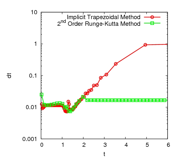
Figure 2: Illustration of the stiffness of Eq. (V) with the $\lambda=2$ sum kernel, Eq. (22). $\Omega$ was taken to be 100, the energy injection rate was $J=1$ and the open truncation was used. The plot compares the timesteps required to keep the numerical solution within an error tolerance of $1\times 10^{-6}$ using the RK2 algorithm and IT method.

The solutions of Eq. (V) exhibit scaling behaviour, with the result that there is a wide variation of the timescale during the course of the evolution. This necessitates Lee (2000) the use of adaptive timestepping to keep the error within a prescribed limit Press et al. (1992). The explicit second order Runge-Kutta (RK2) method and implicit trapezoidal (IT) method were both used in conjunction with a step-doubling procedure to adjust the timestep, $h$. Both have stepwise errors of $O(h^{3})$. The use of an implicit method is necessary for larger values of $\lambda$ because Eq. (V) becomes increasing stiff for larger values of $\lambda$. This is illustrated clearly in Fig. 2 which compares the stepsize required by the explicit RK2 and implicit IT integration algorithms in order to maintain a given error as the solution of Eq. (V) with the sum kernel, Eq. (22) with $\lambda=2$. Initially, the dynamics is fast an both methods require small timesteps to keep the error within the prescribed tolerance. Around $t=2$ the solution approaches the stationary state and the dynamics slows down. The explicit RK2 algorithm continues to require small steps despite the fact that the solution is no longer evolving quickly. In contrast the implicit IT algorithm can take increasingly large steps as the dynamics slows down. This behaviour is the classical symptom of a stiff system and renders explicit solvers practically useless for solving the 3WKE with larger values of $\lambda$.

There is a price to be paid for dealing with the stiffness issue. The IT method requires that we solve the following set of implicit nonlinear equations (we ignore the forcing and dissipation terms for now since they are straightforward to include) to find the energies at the next timestep, $E_{i}(t+h)$, from the energies at the current timestep, $E_{i}(t)$:

$$E_{i}(t+h)=E_{i}(t)+\frac{h}{2}\,\left(S_{i}[{\bf E}(t)]+S_{i}[{\bf E}(t+h)]\right)$$ (71)

This was done using the GSL implementation Galassi et al. (2009) of the Rosenbrock algorithm Rosenbrock (1960), a standard method of multi-dimensional root finding. The current values, $E_{i}(t)$, were used as the initial guess for the root finding procedure.

V.2 Coarse-graining

A direct integration of Eq. (23) is practical only for relatively small numbers of modes. In order to resolve large inertial ranges, we coarse-grain the modes into bins and approximately compute the net energy transfer rate between bins following the approach developed in Lee (2000) for the Smoluchowski equation.

We need to divide the frequency domain, $[1,\Omega)]$, up into $N$ bins. We shall adopt the notation

$$B_{i}=[\omega_{i}^{L},\omega_{i}^{R})$$

to denote the $i^{\rm th}$ bin and denote the bin widths by

$$\Delta\omega_{i}=\omega_{i}^{R}-\omega_{i}^{L}.$$

We use the same bin structure as adopted in Lee (2000): the first $n$ bins are linearly spaced and the next $N-n$ bins are defined by a geometric sequence of boundary points having ratio $a=10^{\frac{1}{n}}$. The final bin is defined so that its right boundary is $\Omega$. With this definition, there are approximately $n$ bins per decade of frequency space with the total number of bins, $N$, determined by the value of the frequency cut-off, $\Omega$. We define a characteristic frequency, $\Omega_{i}$, of each bin by

$$\Omega_{i}=\frac{1}{2}(\omega_{i}^{L}+\omega_{i}^{R}).$$

We shall continue to use $E_{i}$ to denote the total amount of energy contained in bin $i$ despite the fact that for $i>n$ this now refers to an entire bin of frequencies rather than an individual frequency (for the first $n$ bins, each of which contains only a single mode, $E_{i}$ remains just the energy contained in that mode). Likewise we shall continue to use $N_{i}$ to denote the total number of waves in bin $i$. Within each bin, $B_{i}$, with $i>n$ the energy and wave-action distributions within the bin are approximated with power law distributions:

$$e_{i}(\omega) = a_{i}\left(\frac{\omega}{\omega_{i}^{L}}\right)^{b_{i}}\hskip 28.45274pt\omega_{i}^{L}\leq\omega<\omega_{i}^{R}$$ (72)

$$n_{i}(\omega) = a_{i}\left(\frac{\omega}{\omega_{i}^{L}}\right)^{b_{i}-1}.$$ (73)

The exponent, $b_{i}$, is obtained by interpolating the characteristic energies of the neighbouring bins:

$$a_{i}=\frac{\log\left(\frac{E_{i+1}}{\Delta\omega_{i+1}}\right)-\log\left(\frac{E_{i-1}}{\Delta\omega_{i-1}}\right)}{\log\Omega_{i+1}-\log\Omega_{i-1}},$$ (74)

and the prefactor, $a_{i}$, is fixed by the normalisation

$$E_{i}=\int_{\omega_{i}^{L}}^{\omega_{i}^{R}}d\omega\,e_{i}(\omega).$$ (75)

We have seen in Sec. II that computing the collision integral on the RHS of Eq. (23) is equivalent to computing the appropriate rates of energy exchange given by Eq. (17), Eq. (18) and Eq. (19) for the members of each resonant triad and summing over all triads. After course-graining, we need to compute the net rates of energy transfer resulting from the interactions of all triads $(\omega_{i},\omega_{j},\omega_{k})$ for which $\omega_{i}\in B_{i}$ and $\omega_{j}\in B_{j}$ (of course we must allow the possibility that $B_{i}$=$B_{j}$) and sum the results over all possible pairs of bins $B_{i}$ and $B_{j}$. The fundamental quantity which we evolve is naturally the total amount of energy contained in each bin.

When considering interactions between a pair of bins, $B_{j}$ and $B_{k}$, we shall adopt the labeling used in Fig. 1: bin $j$ to the left of bin $k$. In computing the rates of transfer of energy generated by these interactions the first step is to determine which bin or bins contain the modes in resonance with those in $B_{j}$ and $B_{k}$. Before describing how the subsequent energy redistribution works in detail, let us explain the key approximation which will used. Consider, for example, the forward-scatter process. The total rate of energy transfer to higher frequencies due to resonances between modes in $B_{i}$ and $B_{k}$ is given by a double integral,

$$\Delta E = \int_{\omega_{j}^{L}}^{\omega_{j}^{R}}d\omega_{j}\int_{\omega_{k}^{L}}^{\omega_{k}^{R}}d\omega_{k}\,(\omega_{j}+\omega_{k})\,K_{1}(\omega_{j},\omega_{k})$$ (76)

$$\hskip 56.9055pt\,n_{j}(\omega_{j})\,n_{k}(\omega_{k}),$$

and these rates of gain of energy are distributed (non-uniformly) among a set of modes with frequencies lying between $\omega_{j}^{L}+\omega_{k}^{L}$ and $\omega_{j}^{R}+\omega_{k}^{R}$. The key approximation which we make is to treat all modes in $B_{j}$ (the lower frequency narrower bin) as having frequency $\Omega_{j}$ (of course, this is not even an approximation if $j<=n$). That is we replace $n_{j}(\omega_{j})$ with $N_{j}\,\delta(\omega_{j}-\Omega_{j})$ so that instead of computing double integrals, we need to compute one dimensional integrals of the form

$$\Delta E=N_{j}\int_{\omega_{k}^{L}}^{\omega_{k}^{R}}d\omega_{k}\,(\Omega_{j}+\omega_{k})\,K_{1}(\Omega_{j},\omega_{k})\,n_{k}(\omega_{k})$$ (77)

with the gains of energy distributed among a set of modes with frequencies lying between $\Omega_{j}+\omega_{k}^{L}$ and $\Omega_{j}+\omega_{k}^{R}$.

With this approximation in mind, let us now describe explicitly the calculation of the rates of energy transfer. For each pair of bins, $B_{j}$ and $B_{k}$, there are three possibilities which must be treated separately. They are, as listed below, labeled $A$, $B$ and $C$. With apologies for the somewhat clumsy notation, we now list the energy transfer rates to/from each bin for each of these cases split up according to the contributions from each of the processes described by $S_{1}[N_{\omega}]$, $S_{2}[N_{\omega}]$ and $S_{3}[N_{\omega}]$. $L$ shall denote an energy loss term and $G$ an energy gain term. The actual integrals are written explicitly in appendix Appendix: Transfer integrals to avoid an overload of technical details.

• Case A : $k\leq n$
  This is the simplest case in which $B_{k}$ (and hence $B_{j}$) is a discrete bin. Given $j$ and $k$, we identify the bin, $B_{i}$, which contains $\omega_{i}=\Omega_{j}+\Omega_{k}$. Whether it is a discrete or continuous bin is irrelevant. The transfer rates can be read off almost immediately from Eqs. (17), Eqs. (18) and Eqs. (19):

  $$(\Delta E)_{j} = -^{A}L_{j}^{(1)}+^{A}G_{j}^{(2)}+^{A}G_{j}^{(3)}$$

  $$(\Delta E)_{k} = -^{A}L_{k}^{(1)}+^{A}G_{k}^{(2)}+^{A}G_{k}^{(3)}$$ (78)

  $$(\Delta E)_{i} = (\Delta E)_{j}+(\Delta E)_{k}$$

  where

  $${}^{A}L_{j}^{(1)} = \Omega_{j}\,K_{1}(\Omega_{j},\Omega_{k})\,N_{j}\,N_{k}$$

  $${}^{A}L_{k}^{(1)} = \Omega_{k}\,K_{1}(\Omega_{j},\Omega_{k})\,N_{j}\,N_{k}$$

  $${}^{A}G_{j}^{(2)} = \Omega_{j}\,K_{2}(\Omega_{j},\Omega_{k})\,N_{j}\,\frac{N_{i}}{\Delta\omega_{i}}$$

  $${}^{A}G_{k}^{(2)} = \Omega_{k}\,K_{2}(\Omega_{j},\Omega_{k})\,N_{j}\,\frac{N_{i}}{\Delta\omega_{i}}$$

  $${}^{A}G_{j}^{(3)} = \Omega_{j}\,K_{3}(\Omega_{j},\Omega_{k})\,N_{k}\,\frac{N_{i}}{\Delta\omega_{i}}$$

  $${}^{A}G_{k}^{(3)} = \Omega_{k}\,K_{3}(\Omega_{j},\Omega_{k})\,N_{k}\,\frac{N_{i}}{\Delta\omega_{i}}.$$

• Case B : $k>n$ and $[\Omega_{j}+\omega_{k}^{L},\Omega_{j}+\omega_{k}^{R}]$ is contained in a single bin, $B_{i}$
  In this case, we identify the bin, $B_{i}$, which contains all modes in the range $[\Omega_{j}+\omega_{k}^{L},\Omega_{j}+\omega_{k}^{R}]$. The rates of energy transfer are

  $$(\Delta E)_{j} = -^{B}L_{j}^{(1)}+^{B}G_{j}^{(2)}+^{B}G_{j}^{(3)}$$

  $$(\Delta E)_{k} = -^{B}L_{k}^{(1)}+^{B}G_{k}^{(2)}+^{B}G_{k}^{(3)}$$ (79)

  $$(\Delta E)_{i} = (\Delta E)_{j}+(\Delta E)_{k}$$

  with the relevant integrals provided in the appendix.

• Case C : $k>n$ and $[\Omega_{j}+\omega_{k}^{L},\Omega_{j}+\omega_{k}^{R}]$ is split between two bins, $B_{i_{L}}$ and $B_{i_{R}}$
  It can happen that the range of modes $[\Omega_{j}+\omega_{k}^{L},\Omega_{j}+\omega_{k}^{R}]$ spans two bins. With the above definition of the bin structure it is never more than two. We identify these bins as $B_{i_{L}}$ and $B_{i_{R}}$. We must also identify the point $\Omega^{*}=\omega_{i_{R}}^{L}-\Omega_{j}\in B_{k}$ which marks the boundary between those modes in $B_{k}$ which are resonant with modes in $B_{i_{L}}$ and those modes in $B_{k}$ which are resonant with modes in $B_{i_{R}}$. Energy transfer is then split appropriately between $B_{i_{L}}$ and $B_{i_{R}}$:

  $$(\Delta E)_{j} = {}_{L}(\Delta E)_{j}+_{R}(\Delta E)_{j}$$

  $$(\Delta E)_{k} = {}_{L}(\Delta E)_{k}+_{R}(\Delta E)_{k}$$ (80)

  $$(\Delta E)_{i_{L}} = {}_{L}(\Delta E)_{j}+_{L}(\Delta E)_{k}$$

  $$(\Delta E)_{i_{R}} = {}_{R}(\Delta E)_{j}+_{R}(\Delta E)_{k}$$

  where

  $${}_{L}(\Delta E)_{j} = -^{C}_{L}L_{j}^{(1)}+^{C}_{L}G_{j}^{(2)}+^{C}_{L}G_{j}^{(3)}$$

  $${}_{R}(\Delta E)_{j} = -^{C}_{R}L_{j}^{(1)}+^{C}_{R}G_{j}^{(2)}+^{C}_{R}G_{j}^{(3)}$$

  $${}_{L}(\Delta E)_{k} = -^{C}_{L}L_{k}^{(1)}+^{C}_{L}G_{k}^{(2)}+^{C}_{L}G_{k}^{(3)}$$ (81)

  $${}_{R}(\Delta E)_{k} = -^{C}_{R}L_{k}^{(1)}+^{C}_{R}G_{k}^{(2)}+^{C}_{R}G_{k}^{(3)}.$$

  Again, the actual integrals are written explicitly in the appendix.

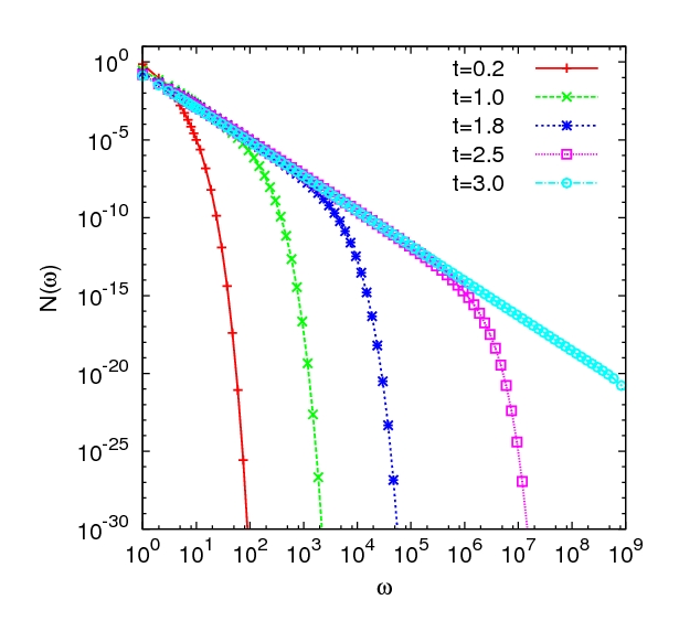
Figure 3: Sample output from implementation the algorithm described in Sec. V. This is a decay simulation with $\lambda=3/2$ product kernel, Eq. (21).

Some typical outputs resulting from the implementation of the algorithm described in this section is shown in Fig. 3.

VI Numerical Validation: Calculation of the Kolmogorov-Zakharov Constant

The evolution of the energy spectrum shown in Fig. 3 certainly looks plausible. Nevertheless, the approximations made in deriving the algorithm described in Sec. V are not systematic and no convergence results have been proven. Therefore it is essential to validate the code. From the discussions of Sec. II, it is obviously inadequate to use the measurement of scaling exponents as a means of validation since the scaling properties of Eq. (11) and Eq. (16) are practically identical even though the physics is very different for the two equations. For Lee’s original implementation of this method for Smoluchowski equation, one had the luxury of several exact solutions Lee (2000); Leyvraz (2003) against which the full time-dependent evolution could be validated. There are, to the best of our knowledge, no known exact solutions of the 3-wave kinetic equation whch could play a similar diagnostic role in the present context. We suggest instead, to use the measurement of the Kolmogorov-Zakharov constant, $c_{\rm KZ}$, as a diagnostic. It can be computed exactly as we shall now show. Furthermore its value is dependent on getting the internal structure of the collision integral correct. Taken together with the measurement of stationary scaling exponents, the measurement of $c_{\rm KZ}$ is a stringent test which the code was required to pass.

Let us now calculate $c_{\rm KZ}$. Consider the statement of conservation of energy,

$$\partial_{t}\left(\omega_{1}N_{\omega_{1}}\right)=\omega_{1}\,S[N_{\omega}]=-\partial_{\omega_{1}}J_{\omega_{1}},$$ (82)

where $J_{\omega}$ is the energy flux at frequency $\omega$. For a general power law spectrum, $N_{\omega}=c\,\omega^{-x}$, we can write the right hand side like Eq. (III.4). Introducing rescaled integration variables, $u$ and $v$ defined by

$$\omega_{2}=\omega_{1}\,v\ \ \ \ \omega_{3}=\omega_{1}\,u,$$

and integrating out $v$ allows us to write Eq. (82) as

$$\partial_{\omega_{1}}J_{\omega_{1}}=-c^{2}\,\omega_{1}^{\lambda-2{\mathbf{x}}+2}\,I(x),$$ (83)

where

$$I(x)=\int_{0}^{1}\left[K_{1}(u,1-u)\,(u(1-u))^{-x}\right.$$ (84)

$$\left.-K_{2}(u,1-u)\,u^{-x}-K_{3}(u,1-u)\,(1-u)^{-x}\right]$$

$$\left[1-(1-u)^{2x-\lambda-2}-u^{2x-\lambda-2}\right]\,du.$$

Integrating once, we get

$$J_{\omega}=-\omega^{\lambda-2x+3}\frac{c^{2}I(x)}{\lambda-2x+3}.$$ (85)

The energy flux, $J_{\omega}$, should be constant, independent of $\omega$, and equal to $J$, the rate of energy injection, when $x$ takes the KZ value, $(\lambda+3)/2$. The limit needs to be taken using l’Hôpital’s Rule since $I(x_{\rm KZ})=0$. The result is

$$J=\frac{1}{2}\,c^{2}\,\left.\frac{dI}{dx}\right|_{x=x_{\rm KZ}}.$$ (86)

The K-Z constant, is therefore given by

$$c_{\rm KZ}=\sqrt{2\,J\,\left.\frac{dI}{dx}\right|_{x=x_{\rm KZ}}^{-1}}$$ (87)

The integral $\left.\frac{dI}{dx}\right|_{x=x_{\rm KZ}}$, can be calculated numerically, and analytically for some interaction coefficients. We shall use this result to validate the numerical solution procedure.

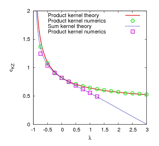
Figure 4: Numerical values of the Kolmogorov–Zakharov constant for the sum kernel, Eq. (22) and the product kernel, Eq. (21), for a range of values of $\lambda$. The theoretical curves come from numerical evaluation of Eq. (87).

Based on the discussion of the previous section, very few properties of the kinetic equation actually depend on $\alpha$ or $d$ and those that do are all related to thermodynamic equilibrium. We shall therefore take $\alpha=d$ so that $K_{1}(\omega_{i},\omega_{j})=K_{2}(\omega_{i},\omega_{j})=K_{3}(\omega_{i},\omega_{j})$. For such systems, the thermodynamic equilibrium spectrum is $\omega^{-1}$. We tested our code with both the product kernel, Eq. (21), and the sum kernel, Eq. (22), for various values of $\lambda$. This was done by allowing the system to reach a stationary state with a constant rate of injection and then compensating the computed spectrum, $N_{\omega}$, with the K-Z spectrum and fitting a constant to the result. The results are shown in Fig. 4. The numerically fitted values of $c_{\rm KZ}$ are in excellent agreement with the theoretical predictions obtained from Eq. (87) for both kernels which gives us confidence in the numerical algorithm introduced in Sec. V. Note that the value of the $c_{\rm KZ}$ diverges at $\lambda=-1$ for both kernels. This comes from the fact that, in the numerics we took $\alpha=d$ so the the thermodynamic spectrum, Eq. (44) has exponent $x=1$. Thus at $\lambda=-1$ the thermodynamic and K-Z exponents coincide. From the locality conditions, Eq. (61), derived in Sec. III, we know that the collision integral diverges when this occurs due to the violation of the first condition in Eq. (61). Notice also that the vanishing of $c_{\rm KZ}$ for the sum kernel at $\lambda=3$ corresponds to the breakdown of locality due to the violation of the second condition in Eq. (61). Fig. 4 therefore provides a nice consistency check on our earlier theoretical analysis.

VII Finite and Infinite Capacity Cascades and Dissipative Anomaly

The concept of a dissipative anomaly is key to understanding the statistical properties of many turbulent systems. It refers to a situation in which the average rate of energy dissipation tends to become independent of the dissipation parameter in the dynamical equations in the limit where this dissipation parameter is taken to zero. This phenomenon is explicitly demonstrable in Burgers’ equation (see Bec and Khanin (2007) for a review) where the rate of dissipation of energy in shocks becomes independent of the viscosity, $\nu$, as $\nu\to 0$. It is also believed to be very relevant (see the discussion in Eyink (2008)) for the high Reynolds number limit of hydrodynamic turbulence.

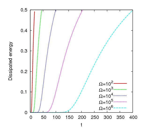
Figure 5: Time dependence of the dissipated energy for increasing values of the dissipation scale, $\Omega$, for the product kernel, Eq. (21) with $\lambda=\frac{3}{4}$.

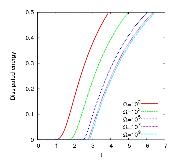
Figure 6: Time dependence of the dissipated energy for increasing values of the dissipation scale, $\Omega$, for the product kernel, Eq. (21) with $\lambda=\frac{3}{2}$.

In wave turbulence it is expected that the dissipative anomaly is present for finite capacity wave systems and absent for infinite capacity systems. In Sec. III we showed that $\lambda=1$ is the boundary between infinite and finite capacity. The difference between the two can be explicitly demonstrated using the numerical scheme developed in Sec. V. We have seen that an open truncation of the 3 wave kinetic equation introduces dissipation of energy with the dissipation scale given by $\Omega$, the cut-off frequency. The non-dissipative limit in this situation corresponds to taking this dissipative cut-off to infinity. Figs. 5 and 6 show the total dissipated energy as a function of time for two decay systems with the same initial condition, $N_{\omega}(0)=\delta(\omega-1)$, interacting via the product kernel, Eq. (21) with two different values of $\lambda$. Fig. 5 shows total dissipated energy as a function of time for the case $\lambda=3/4$ which is infinite capacity. As the cut-off, $\Omega$, is increased the time at which the energy is dissipated increases. Consequentially, the dissipated energy at any fixed time vanishes as the dissipative cut-off is removed to infinity. Hence there is no dissipative anomaly. The corresponding situation for the finite capacity case, $\lambda=3/2$, shown in Fig. 6 is strikingly different. As the dissipative cut-off, $\Omega$, is removed, the dissipated energy as a function of time becomes independent of $\Omega$. From the figure it is clear that for times larger than about 3, the dissipated energy is finite in the limit $\omega\to\infty$. This is as explicit a demonstration as one may expect from a numerical simulation of the presence of a dissipative anomaly in this system.

It is worth noting that the corresponding dissipative anomaly for the Smoluchowski kinetic equation is well known in the aggregation literature where it is more commonly referred to as the gelation transition. The criterion, $\lambda>1$, is common to both systems. A numerical study similar to what has been presented here is provided for that system in Connaughton et al. (2009). An exact solution for the Smoluchowski equation with the product kernel which exhibits the anomaly explicitly can be found in Sec. 4.5 of Leyvraz (2003). In the light of the numerical results presented here, the construction of the corresponding mathematically rigorous solution of the 3-wave kinetic equation would likely be a fruitful line of research.

VIII The Bottleneck Effect in Systems With Open Truncation

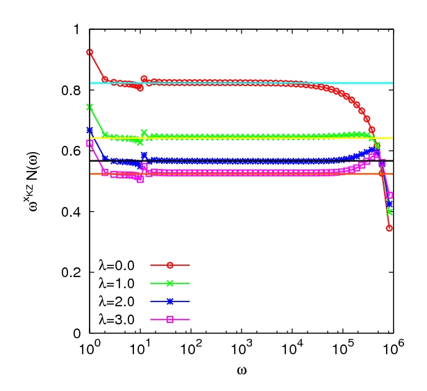
Figure 7: The bottleneck effect in the 3-wave kinetic equation with constant energy injection at $\omega=1$ and open truncation at $\Omega=10^{6}$. The plot shows stationary spectra compensated by the K-Z scaling for the product kernel, Eq. (21), for a range of values of $\lambda$. The bottleneck effect results in an accumulation or depletion of the spectrum near the cut-off, depending on the choice of kernel. Solid lines indicate the theoretically predicted values of the K-Z constant from Eq. (87).

In the previous section, we were interested in the bahaviour of the solution of the 3-wave kinetic equation with open truncation at fixed time as the dissipative cut-off, $\Omega$, tends to infinity. In this section, we shall consider the complementary situation where $\Omega$ is fixed and time tends to infinity. In this situation, irrespective of whether there is a dissipative anomaly or not, we always expect the solution to tend to a stationary state corresponding to the Kolmogorov–Zakharov spectrum, Eq. (33), modified by the presence of the finite cut-off. A question of interest is how the K-Z spectrum matches to the dissipation range and the first issue which arises is whether or not there is a “bottleneck” effect.

The term “bottleneck” refers to a phenomenon, initially observed in numerical simulations of Navier–Stokes turbulence (see Dobler et al. (2003) and the references therein) where the stationary spectrum exhibits a “bump” super-imposed upon the expected constant flux spectrum as it enters the dissipation range. A pysical mechanism for the bottleneck was suggested in Falkovich (1994). A corresponding theory for the wave turbulence case was suggested in Falkovich and Ryzhenkova (1990). It is an intrinsically dissipative phenomenon. It arises because the rate of forward transfer of energy from frequency $\omega_{1}$ due to the interaction with frequency $\omega_{2}>\omega_{1}$ is proportional to the product, $N_{\omega_{1}}N_{\omega_{2}}$, of occupation numbers of both frequencies (see Eq. (17)). The $\omega_{2}$ contributing to the total rate of transfer of energy can be divided into those $\omega_{2}$ less than the dissipative scale, $\Omega$, and those greater than $\Omega$. The latter set are in the dissipative range, where $N_{\omega_{2}}$ is effectively zero (exactly zero in the case of dissipation via an open truncation as is considered in this article). Therefore the rate of forward transfer of energy through $\omega_{1}$ would be decreased. However since $\omega_{1}$ is still in the inertial range, the rate of energy transfer must remain equal to the injected flux. Hence the occupation numbers of those $\omega_{2}$ between $\omega_{1}$ and $\Omega$ must increase so that the same flux can be carried by fewer triads (hence the term “bottleneck”). This effect then produces the bump at the end of the spectrum.

Here we investigate the bottleneck effect in the 3-wave kinetic equation explicitly using the numerical algorithm developed in Sec. V. Fig. 7 shows some results. We computed the stationary state of Eq. (11) with an open truncation at $\Omega=10^{6}$ and the product kernel, Eq. (21) for several different values of $\lambda$. Fig. 7 shows several such stationary spectra compensated by the corresponding K-Z spectra. The solid lines indicate the fitted values of the K-Z constant used for validation of the code in Sec. VI. We see that there is non-trivial structure super-imposed upon the K-Z spectrum as it approaches the dissipative cut-off. Interestingly, whether this structure corresponds to a bump or not depends upon the value of $\lambda$. The heuristic argument outlined above might lead one to expect that the bottleneck effect always produces a bump whereas, in reality, this does not seem to be the case. From the numerical calculations, it seems that the matching of the spectrum to the dissipation produces a bump for $\lambda>1$ but produces a hollow for $\lambda<1$. We shall remain agnostic on the question of whether it is appropriate to call each of these regimes a bottleneck. While this is not a systematic study, it suggests that it might be worthwhile to revisit the bottleneck phenomenon in wave turbulence.

IX Thermalisation in Systems with Closed Truncation

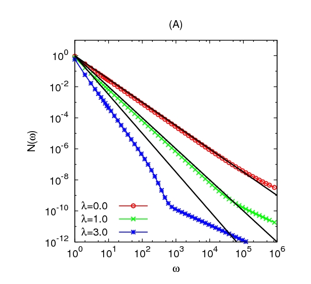
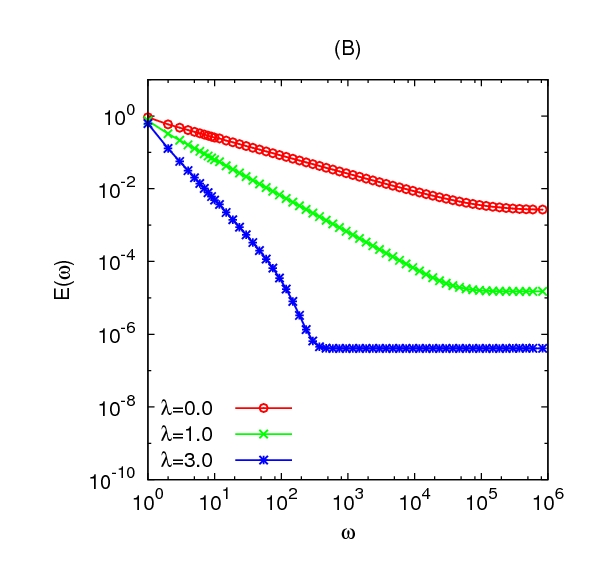
Figure 8: Thermalisation in decay simulations of the 3-wave kinetic equation, Eq. (11), with closed truncation ($\gamma=0$) at $\Omega=10^{6}$ for the product kernel, Eq. (21), for several different values of $\lambda$. The left panel shows the wave spectrum, $N_{\omega}$, and the right panel shows the corresponding energy distribution, $E_{\omega}$, from which the equipartition effect near the cut-off is clear.

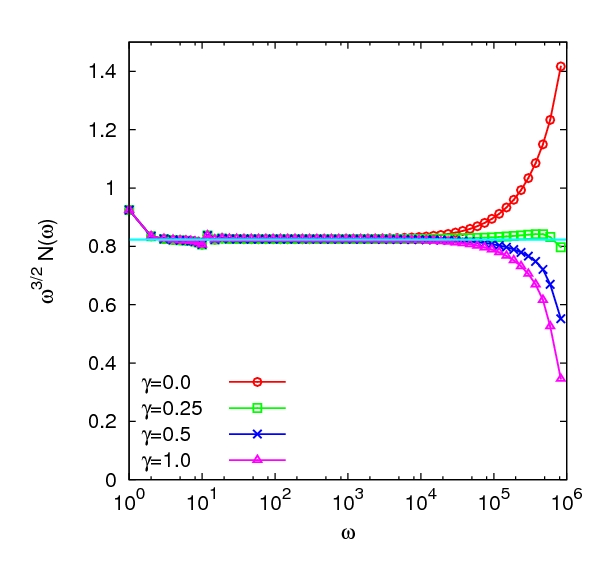
Figure 9: Partial thermalisation in the 3-wave kinetic equation, Eq. (11), with constant kernel and a partially open truncation at $\Omega=10^{6}$. The plot shows stationary spectra (with the exception of the case $\gamma=0$ for which there is no stationary state) compensated by the K-Z scaling $\omega^{3/2}$ for several different values of $\gamma$.

In the previous two sections, we investigated two phenomena - the dissipative anomaly and the bottleneck effect - which were related to the choice of open truncation. In this section we consider the 3-wave kinetic equation with closed truncation where a new phenomenon arises known as thermalisation.

We have already seen that Eq. (5) has two stationary scaling solutions - a thermodynamic solution and a KZ solution. The former has finite temperature and zero energy flux whereas the latter has finite energy flux and zero temperature. It is conjectured Zakharov et al. (1992); Dyachenko et al. (1992) that the general solution of Eq. (5) should be a two-parameter function depending on both a flux and a temperature although little is known about what such mixed states should look like except, perhaps, as pertubations of the pure K-Z or pure thermodynamic solutions (see chap. 4 of Zakharov et al. (1992)). They were first realised in Connaughton and Nazarenko (2004) in the context of the Leith model - a very simplified model of hydrodynamic turbulence - and soon after were properly observed in the full Euler equations Cichowlas et al. (2005). Since then, considerable effort has been invested in understanding the interplay between thermalisation and turbulence in the hydrodynamic context Frisch et al. (2008); Bos and Bertoglio (2006); Krstulovic et al. (2008) where it is argued Frisch et al. (2008) that the closed truncation arises naturally. Despite all of this activity, the phenomenon has not yet been investigated in the context of wave turbulence.

In order for thermalisation to be possible, the energy of the truncated system should be conserved. Following the discussion of Sec. IV, we should choose $\gamma=0$ in Eq. (62) and work with the closed truncation. We performed a series of decay calculations of Eq. (62) with initial condition $N_{\omega}=\delta(\omega-1)$ and truncation frequency $\Omega=10^{6}$ for the product kernel, Eq. (21), with a range of values of $\lambda$. Some representative results are shown in Fig. 8. Since these are decay simulations, the spectra shown in Fig. 8 are not stationary. The spectra are presented at times for which the corresponding system with an open truncation would have dissipated half of the initial energy. Thus the results of Fig. 8 are directly comparable with the decay simulations used to investigate the dissipative anomaly in Sec. VII. Fig. 8(A) shows the spectra for several different values of $\lambda$. The solid black lines indicate the corresponding K-Z spectra. The effect of the closed truncation is clearly evident in the increase of the spectrum above its K-Z value near the cut-off. That this corresponds to thermalisation of the high frequencies is evident from Fig. 8(B) which shows the corresponding energy spectra. It is clear that that the spectrum is crossing over to an equipartition of energy near the cut-off.

Unlike the dissipative bottleneck associated with the open truncation which we studied in Sec. VIII, thermalisation always leads to an accumulation of energy near the cut-off, irrespective of the interaction coefficient. The distinction is clearly illustrated by comparing the $\lambda=0$ cases for the closed and open truncations. The closed truncation leads to accumulation of energy near the cut-off as shown in Fig. 8(A) whereas the open truncation leads to depletion of energy near the cut-off as shown in Fig. 7. Since thermalisation always leads to accumulation of energy near the cut-off, this effect is sometimes also referred to as a “bottleneck”. In the current study, such dual use of terminology would be quite confusing since the closed truncation leading to thermalisation has, by construction, zero flux at $\omega=\Omega$. On the other hand, the open truncation leading to the bottleneck effect has, by construction, a finite flux at $\omega=\Omega$.

The two phenomena can be linked to each other using the partially open truncation discussed in Sec. IV. Although it seems unlikely that such a boundary condition is of much relevance to any physical system, choosing the parameter $\gamma$ in Eq. (11) to have intermediate values between 0 and $1$ allows us to interpolate smoothly between the open and closed truncation and hence between small scale thermalisation and small scale bottleneck. The results of one such exercise in numerical trickery is shown in Fig. 9. In this figure, spectra compensated by the K-Z scaling are shown which were obtained by solving Eq. (11) with constant kernel ($\lambda=0$) and several different values of $\gamma$ for a system truncated at $\Omega=10^{6}$. The spectra shown for the finite $\gamma$ are truly stationary. Unlike the spectra in Fig. 8 discussed above, the spectra in Fig. 9 were obtained with a forcing term injecting energy at a constant rate. Obviously this was not possible for the case $\gamma=0$ where the total energy diverges in the forced case. The spectrum for $\gamma$ is not stationary and is displayed at a time which allows it to be compared with the other spectra. The message to be taken from Fig. 8 is that the depletion of energy near the cut-off due to the open cut-off goes over to a thermalised accumulation of energy near the cut-off as the efficiency of the dissipation is decreased. It would be interesting to investigate the relationship between the open and closed truncations more carefully, especially to understand the role played by the interaction coefficient in determining the shape of the spectrum near the cut-off.

X Conclusions

To conclude, we have outlined an analogy between the isotropic 3-wave kinetic equation and the rate equations for a aggregation–fragmentation problem with an unusual nonlinear fragmentation mechanism. This analogy demonstrates that almost all properties of the system are determined by a single scaling parameter, $\lambda=\frac{2\beta-\alpha}{\alpha}$ thus greatly reducing the parameter space of possible behaviours. A new numerical scheme was constructed based on this analogy which allows for the stable integration of the isotropic 3-wave kinetic equation over many decades of frequency space. This algorithm was validated by comparing numerical measurements of the stationary state with theoretical calculations of the K-Z constant for a range of model interaction coefficients. Several applications of the new algorithm were then presented including studies of the dissipative anomaly, bottleneck effect and thermalisation phenomenon.

The preliminary results presented here by way of motivation for the study of the isotropic 3-wave kinetic equation have suggested that some further investigation of cut-off related phenomena such as the bottleneck would likely be fruitful. In addition, since the initial studies of Galtier et al. Galtier et al. (2000) of the solutions of the Alfven wave kinetic equation, there is growing evidence Lee (2001); Connaughton et al. (2003b); Connaughton and Nazarenko (2004) that finite capacity cascade often, if not always, exhibit a dynamical scaling anomaly during the transient stage of evolution which cannot be understood from elementary scaling arguments. The methods developed in this article should provide an ideal set of tools to study this phenomenon in the setting of general kinetic equations. This will form the basis of future work. The other obvious line or research which has opened up is the question of whether the methods decribed here can be extended to the case of the isotropic 4-wave kinetic equation. At this point, the answer does not seem obvious. The key approximation used in Sec. V to develop the numerical algorithm involved treating all waves in the leftmost bin as having the same frequency. This may not be a reasonable approximation in a 4-wave system where the waves interact in quartets and the possibility of an inverse cascade may increase the sensitivity of the dynamics to the way in which low frequencies are approximated.

XI Acknowlegements

The author acknowledges helpful discussions with E. Ben-Naim, P. Krapivsky, Y. Lvov, A.C. Newell and Y. Pomeau and thanks F. Leyvraz for bringing the work of M.H. Lee to his attention.

Appendix: Derivation of the Aggregation–Fragmentation Equations

We consider isotropic wave turbulence. The wave spectrum , $n_{\mathbf{k}}$, is therefore a function of $k=\left|{\mathbf{k}}\right|$ only which we shall denote by $n_{k}$. There exist a strightforward set of changes of variables which take advantage of this isotropy to convert the collision integral over the pair of $d$–dimensional wave-vectors, ${\mathbf{k}}_{1}$ and ${\mathbf{k}}_{2}$, into one-dimensional integrals over frequencies.

The total number of waves in the system is

$$N=\int_{{\mathbb{R}}^{d}}n_{\mathbf{k}}\,d{\mathbf{k}}.$$

Denoting the radial coordinate of ${\mathbf{k}}\in{\mathbb{R}}^{d}$ and integration over the corresponding angular variables by $d\Theta^{(d)}_{\mathbf{k}}$ we can write this integral in spherical polar co-ordinates as:

$$N = \int_{0}^{\infty}k^{d-1}\,dk\int d\Theta^{(d)}_{\mathbf{k}}n_{\mathbf{k}}$$

$$= \Omega^{(d)}\int_{0}^{\infty}n_{k}k^{d-1}dk$$

where we have used the isotropy of $n_{\mathbf{k}}$ to integrate over the angular variables and denoted the resulting $d$-dimensional solid angle by $\Omega^{(d)}$. We now use the isotropy of the dispersion relation,

$$\omega({\mathbf{k}})=c\,k^{\alpha}$$

to change variables from integration over $k$ to integration over $\omega$:

$$N = \Omega^{(d)}\int_{0}^{\infty}n_{k}k^{d-1}\frac{dk}{d\omega}d\omega$$ (88)

$$= \frac{\Omega^{(d)}}{\alpha}\,c^{-\frac{\alpha}{d}}\int_{0}^{\infty}n_{\omega}\,\omega^{\frac{d-\alpha}{\alpha}}\,d\omega.$$

where $n_{\omega}=n_{k(\omega)}$. Based on these manipulations, we define the angle-averaged frequency spectrum, $N_{\omega}$, by

$$N_{\omega}=\frac{\Omega^{(d)}}{\alpha}\,c^{-\frac{\alpha}{d}}\omega^{\frac{d-\alpha}{\alpha}}\,n_{\omega}$$ (89)

The angle-averaged frequency spectrum has the advantage that the total number of waves, $N$, and total wave energy, $E$, are given very simply as

$$N = \int_{0}^{\infty}N_{\omega}\,d\omega$$ (90)

$$E = \int_{0}^{\infty}\omega N_{\omega}\,d\omega.$$ (91)

Our objective is to integrate over angular variables and express the kinetic equation entirely in terms of $N_{\omega}$.

We begin by using Eq. (5), to write an evolution equation for the time evolution of $N_{\omega_{1}}$:

$$\int_{0}^{\infty}\frac{\partial N_{\omega_{1}}}{\partial t}d\omega_{1} = \int_{\mathbb{R}}^{d}S[n_{\mathbf{k}}]\,d{\mathbf{k}}_{1}$$

$$\equiv \int_{0}^{\infty}(S_{1}[N_{\omega}]+S_{2}[N_{\omega}]+S_{3}[N_{\omega}])\,d\omega_{1}.$$

This yields a kinetic equation of the form

$$\frac{\partial N_{\omega_{1}}}{\partial t}=S_{1}[N_{\omega}]+S_{2}[N_{\omega}]+S_{3}[N_{\omega}].$$ (92)

To determine the form of $S_{1}[N_{\omega}]$, $S_{2}[N_{\omega}]$ and $S_{3}[N_{\omega}]$ we split the collision integral, $S[n_{\mathbf{k}}]$, into three terms, as follows:

$$\int_{{\mathbb{R}}^{d}}S[n_{{\mathbf{k}}}]d{\mathbf{k}}_{1}=a_{1}T_{1}+a_{2}T_{2}+a_{3}T_{3}$$

$$= 4\pi\int L_{{\mathbf{k}}_{1}{\mathbf{k}}_{2}{\mathbf{k}}_{3}}^{2}(a_{1}n_{{\mathbf{k}}_{2}}n_{{\mathbf{k}}_{3}}-a_{2}n_{{\mathbf{k}}_{1}}n_{{\mathbf{k}}_{3}}-a_{3}n_{{\mathbf{k}}_{1}}n_{{\mathbf{k}}_{2}})$$

$$\hskip 14.22636pt\delta(\omega_{{\mathbf{k}}_{1}}-\omega_{{\mathbf{k}}_{2}}-\omega_{{\mathbf{k}}_{3}})\,\delta({\mathbf{k}}_{1}-{\mathbf{k}}_{2}-{\mathbf{k}}_{3})\,d{\mathbf{k}}_{1}d{\mathbf{k}}_{2}d{\mathbf{k}}_{3}$$

$$- 4\pi\int L_{{\mathbf{k}}_{2}{\mathbf{k}}_{3}{\mathbf{k}}_{1}}^{2}(a_{1}n_{{\mathbf{k}}_{1}}n_{{\mathbf{k}}_{3}}-a_{2}n_{{\mathbf{k}}_{2}}n_{{\mathbf{k}}_{3}}-a_{3}n_{{\mathbf{k}}_{1}}n_{{\mathbf{k}}_{2}})$$

$$\hskip 14.22636pt\delta(\omega_{{\mathbf{k}}_{2}}-\omega_{{\mathbf{k}}_{3}}-\omega_{{\mathbf{k}}_{1}})\,\delta({\mathbf{k}}_{2}-{\mathbf{k}}_{3}-{\mathbf{k}}_{1})\,d{\mathbf{k}}_{1}d{\mathbf{k}}_{2}d{\mathbf{k}}_{3}$$

$$- 4\pi\int L_{{\mathbf{k}}_{3}{\mathbf{k}}_{1}{\mathbf{k}}_{2}}^{2}(a_{1}n_{{\mathbf{k}}_{1}}n_{{\mathbf{k}}_{2}}-a_{2}n_{{\mathbf{k}}_{1}}n_{{\mathbf{k}}_{3}}+a_{3}n_{{\mathbf{k}}_{2}}n_{{\mathbf{k}}_{3}})$$

$$\hskip 14.22636pt\delta(\omega_{{\mathbf{k}}_{3}}-\omega_{{\mathbf{k}}_{1}}-\omega_{{\mathbf{k}}_{2}})\,\delta({\mathbf{k}}_{3}-{\mathbf{k}}_{1}-{\mathbf{k}}_{2})\,d{\mathbf{k}}_{1}d{\mathbf{k}}_{2}d{\mathbf{k}}_{3}$$

The variables $a_{1}=a_{2}=a_{3}=1$ have been introduced simply to indicate which terms are to be grouped together.

Let us first consider the terms proportional to $a_{1}$. We again introduce spherical polar coordinates:

$$\int d{\mathbf{k}}_{1}d{\mathbf{k}}_{2}d{\mathbf{k}}_{3}=\int(k_{1}k_{2}k_{3})^{d-1}d\Theta^{(d)}_{\mathbf{k}_{1}}d\Theta^{(d)}_{\mathbf{k}_{2}}d\Theta^{(d)}_{\mathbf{k}_{3}}dk_{123},$$ (94)

where the notation $dk_{123}$ represents the integration measure, $dk_{1}dk_{2}dk_{3}$, over the radial variables. Noting that the angular variables only enter into the interaction coefficients, $L_{{\mathbf{k}}_{1}{\mathbf{k}}_{2}{\mathbf{k}}_{3}}$ and the ${\mathbf{k}}$ delta functions, we can define an angle-averaged interaction coefficient,

$$\widetilde{L}(k_{1},k_{2},k_{3}) = 4\pi\int L_{{\mathbf{k}}_{1}{\mathbf{k}}_{2}{\mathbf{k}}_{3}}^{2}\delta({\mathbf{k}}_{1}\!-\!{\mathbf{k}}_{2}\!-\!{\mathbf{k}}_{3})$$

$$\hskip 28.45274ptd\Theta^{(d)}_{\mathbf{k}_{1}}d\Theta^{(d)}_{\mathbf{k}_{2}}d\Theta^{(d)}_{\mathbf{k}_{3}},$$

which is a function of the radial variables only. We can then write

$$T_{1} = \int\widetilde{L}_{k_{1}k_{2}k_{3}}\,n_{k_{2}}n_{k_{3}}(k_{1}k_{2}k_{3})^{d-1}\,\delta(\omega^{1}_{23})\,dk_{123}$$

$$- \int\widetilde{L}_{k_{2}k_{3}k_{1}}\,n_{k_{1}}n_{k_{3}}(k_{1}k_{2}k_{3})^{d-1}\,\delta(\omega^{2}_{31})\,dk_{123}$$

$$- \int\widetilde{L}_{k_{3}k_{1}k_{2}}\,n_{k_{1}}n_{k_{2}}(k_{1}k_{2}k_{3})^{d-1}\,\delta(\omega^{3}_{12})\,dk_{123}.$$

Here the notation $\delta(\omega^{i}_{jk})$ is a compact representation of the frequency delta function:

$$\delta(\omega^{i}_{jk})=\delta(\omega_{i}-\omega_{j}-\omega_{k}).$$ (96)

Now replace the integration over $k$’s with integration over frequencies as we did in Eq. (88) and use Eq. (89) to express $n_{\omega}$ in terms of $N_{\omega}$. The result is

$$T_{1} = c_{d}\int\bar{L}_{\omega_{1}\omega_{2}\omega_{3}}\,\omega_{1}^{\frac{d-\alpha}{\alpha}}\,N_{\omega_{2}}N_{\omega_{3}}\delta(\omega^{1}_{23})\,d\omega_{123}$$

$$- c_{d}\int\bar{L}_{\omega_{2}\omega_{3}\omega_{1}}\,\omega_{2}^{\frac{d-\alpha}{\alpha}}\,N_{\omega_{1}}N_{\omega_{3}}\delta(\omega^{2}_{31})\,d\omega_{123}$$

$$- c_{d}\int\bar{L}_{\omega_{3}\omega_{1}\omega_{2}}\,\omega_{3}^{\frac{d-\alpha}{\alpha}}\,N_{\omega_{1}}N_{\omega_{2}}\delta(\omega^{3}_{12})\,d\omega_{123},$$

where

$$\bar{L}_{\omega_{1}\omega_{2}\omega_{3}} = \widetilde{L}_{\left(\frac{\omega_{1}}{c}\right)^{\frac{1}{\alpha}}\left(\frac{\omega_{2}}{c}\right)^{\frac{1}{\alpha}}\left(\frac{\omega_{3}}{c}\right)^{\frac{1}{\alpha}}}$$ (98)

$$c_{d} = \frac{c^{\frac{4-d}{\alpha}}}{\alpha{\Omega^{(d)}}^{2}}.$$

Finally define

$$K_{1}(\omega_{i},\omega_{j})=c_{d}\bar{L}_{\omega_{i}+\omega_{j}\,\omega_{i}\omega_{j}}\,(\omega_{i}+\omega_{j})^{\frac{d-\alpha}{\alpha}}.$$ (99)

Now use the frequency delta-functions to write Eq (Appendix: Derivation of the Aggregation–Fragmentation Equations) as

$$T_{1} = \int K_{1}(\omega_{2},\omega_{3})\,N_{\omega_{2}}N_{\omega_{3}}\delta(\omega^{1}_{23})\,d\omega_{123}$$

$$- \int K_{1}(\omega_{3},\omega_{1})\,N_{\omega_{1}}N_{\omega_{3}}\delta(\omega^{2}_{31})\,d\omega_{123}$$

$$- \int K_{1}(\omega_{1},\omega_{2})\,N_{\omega_{1}}N_{\omega_{2}}\delta(\omega^{3}_{12})\,d\omega_{123},$$

Comparing with Eq. (Appendix: Derivation of the Aggregation–Fragmentation Equations) we see that we should write

$$S_{1}[N_{\omega}]\!\!\! = \!\!\!\!\!\int\!\!K_{1}(\omega_{2},\omega_{3})\,N_{\omega_{2}}N_{\omega_{3}}\delta(\omega_{1}\!-\!\omega_{2}\!-\!\omega_{3})\,d\omega_{23}$$

$$- \!\!\!\!\!\int\!\!K_{1}(\omega_{3},\omega_{1})\,N_{\omega_{1}}N_{\omega_{3}}\delta(\omega_{2}\!-\!\omega_{3}\!-\!\omega_{1})\,d\omega_{23}$$

$$- \!\!\!\!\!\int\!\!K_{1}(\omega_{1},\omega_{2})\,N_{\omega_{1}}N_{\omega_{2}}\delta(\omega_{3}\!-\!\omega_{1}\!-\!\omega_{2})\,d\omega_{23}.$$

The same set of manipulations can now be applied to the terms proportional to $a_{2}$ and $a_{3}$ in Eq. (Appendix: Derivation of the Aggregation–Fragmentation Equations) to deduce the appropriate forms of $S_{2}[N_{\omega}]$ and $S_{3}[N_{\omega}]$. The results are as follows:

$$S_{2}[N_{\omega}]\!\!\! = \!\!\!\!\!\int\!\!K_{2}(\omega_{2},\omega_{3})\,N_{\omega_{1}}N_{\omega_{3}}\delta(\omega_{1}\!-\!\omega_{2}\!-\!\omega_{3})\,d\omega_{23}$$

$$- \!\!\!\!\!\int\!\!K_{2}(\omega_{3},\omega_{1})\,N_{\omega_{2}}N_{\omega_{3}}\delta(\omega_{2}\!-\!\omega_{3}\!-\!\omega_{1})\,d\omega_{23}$$

$$- \!\!\!\!\!\int\!\!K_{2}(\omega_{1},\omega_{2})\,N_{\omega_{1}}N_{\omega_{3}}\delta(\omega_{3}\!-\!\omega_{1}\!-\!\omega_{2})\,d\omega_{23}$$

and

$$S_{3}[N_{\omega}]\!\!\! = \!\!\!\!\!\int\!\!K_{3}(\omega_{2},\omega_{3})\,N_{\omega_{1}}N_{\omega_{2}}\delta(\omega_{1}\!-\!\omega_{2}\!-\!\omega_{3})\,d\omega_{23}$$

$$- \!\!\!\!\!\int\!\!K_{3}(\omega_{3},\omega_{1})\,N_{\omega_{1}}N_{\omega_{2}}\delta(\omega_{2}\!-\!\omega_{3}\!-\!\omega_{1})\,d\omega_{23}$$

$$- \!\!\!\!\!\int\!\!K_{3}(\omega_{1},\omega_{2})\,N_{\omega_{2}}N_{\omega_{3}}\delta(\omega_{3}\!-\!\omega_{1}\!-\!\omega_{2})\,d\omega_{23}.$$

Note that there is a small price to be paid for hiding all dependence on $d$ and $\alpha$: the interaction coefficients for the three collision integrals are, in general, not identical:

$$K_{2}(\omega_{i},\omega_{j}) = K_{1}(\omega_{i},\omega_{j})\left(\frac{\omega_{i}+\omega_{j}}{\omega_{j}}\right)^{\frac{\alpha-d}{\alpha}}$$

$$K_{3}(\omega_{i},\omega_{j}) = K_{1}(\omega_{i},\omega_{j})\left(\frac{\omega_{i}+\omega_{j}}{\omega_{i}}\right)^{\frac{\alpha-d}{\alpha}}.$$ (104)

Note also that $K_{2}(\omega_{i},\omega_{j})$ and $K_{3}(\omega_{i},\omega_{j})$, are not symmetric in their arguments although this latter deficiency can be removed if desired by symmetrisation. These problems are immaterial since the original variables can be easily restored if needs be. It is worth noting that in the case where $d=\alpha$, the distinctions between the interaction coefficients disappear. Furthermore, even in the general case, all three interaction coefficients have the same degree of homogeneity. From Eq. (99), Eq. (98) and Eq. (Appendix: Derivation of the Aggregation–Fragmentation Equations), it is easy to work backwards and establish that this degree of homogeneity, which we denote by $\lambda$, is

$$\lambda=\frac{2\beta-\alpha}{\alpha}.$$ (105)

Thus, if one is interested in scaling properties of 3-wave kinetic equation, almost everything is determined by this single scaling parameter, $\lambda$.

Appendix: Transfer integrals

In this appendix we state the explicit expressions for the various transfer integrals which go into the estimation of the collision integral according to Eq. (79) and Eq. (80).

• Case B :
  

  $${}^{B}L_{j}^{(1)} = \Omega_{j}\,N_{j}\int_{\omega_{k}^{L}}^{\omega_{k}^{R}}K_{1}(\Omega_{j},\omega_{k})\,n_{k}(\omega_{k})\,dw_{k}$$

  $${}^{B}L_{k}^{(1)} = N_{j}\int_{\omega_{k}^{L}}^{\omega_{k}^{R}}\omega_{k}\,K_{1}(\Omega_{j},\omega_{k})\,n_{k}(\omega_{k})\,dw_{k}$$

  $${}^{B}G_{j}^{(2)} = \Omega_{j}\,N_{j}\int_{\omega_{k}^{L}}^{\omega_{k}^{R}}K_{2}(\Omega_{j},\omega_{k})\,n_{i}(\Omega_{j}+\omega_{k})$$

  $${}^{B}G_{k}^{(2)} = N_{j}\int_{\omega_{k}^{L}}^{\omega_{k}^{R}}\omega_{k}\,K_{2}(\Omega_{j},\omega_{k})\,n_{i}(\Omega_{j}+\omega_{k})$$

  $${}^{B}G_{j}^{(3)} = \Omega_{j}\,\Delta\omega_{j}\int_{\omega_{k}^{L}}^{\omega_{k}^{R}}K_{3}(\Omega_{j},\omega_{k})\,n_{k}(\omega_{k})\,n_{i}(\Omega_{j}+\omega_{k})$$

  $${}^{B}G_{k}^{(3)} = \Delta\omega_{j}\int_{\omega_{k}^{L}}^{\omega_{k}^{R}}\omega_{k}\,K_{3}(\Omega_{j},\omega_{k})\,n_{k}(\omega_{k})\,n_{i}(\Omega_{j}+\omega_{k})$$

• Case C :
  

  $${}_{L}^{C}L_{j}^{(1)} = \Omega_{j}\,N_{j}\int_{\omega_{k}^{L}}^{\Omega^{*}}K_{1}(\Omega_{j},\omega_{k})\,n_{k}(\omega_{k})\,dw_{k}$$

  $${}_{L}^{C}L_{k}^{(1)} = N_{j}\int_{\omega_{k}^{L}}^{\Omega^{*}}\omega_{k}\,K_{1}(\Omega_{j},\omega_{k})\,n_{k}(\omega_{k})\,dw_{k}$$

  $${}_{L}^{C}G_{j}^{(2)} = \Omega_{j}\,N_{j}\int_{\omega_{k}^{L}}^{\Omega^{*}}K_{2}(\Omega_{j},\omega_{k})\,n_{i_{L}}(\Omega_{j}+\omega_{k})$$

  $${}_{L}^{C}G_{k}^{(2)} = N_{j}\int_{\omega_{k}^{L}}^{\Omega^{*}}\omega_{k}\,K_{2}(\Omega_{j},\omega_{k})\,n_{i_{L}}(\Omega_{j}+\omega_{k})$$

  $${}_{L}^{C}G_{j}^{(3)} = \Omega_{j}\,\Delta\omega_{j}\int_{\omega_{k}^{L}}^{\Omega^{*}}K_{3}(\Omega_{j},\omega_{k})\,n_{k}(\omega_{k})\,n_{i_{L}}(\Omega_{j}+\omega_{k})$$

  $${}_{L}^{C}G_{k}^{(3)} = \Delta\omega_{j}\int_{\omega_{k}^{L}}^{\Omega^{*}}\omega_{k}\,K_{3}(\Omega_{j},\omega_{k})\,n_{k}(\omega_{k})\,n_{i_{L}}(\Omega_{j}+\omega_{k})$$

  $${}_{R}^{C}L_{j}^{(1)} = \Omega_{j}\,N_{j}\int_{\Omega^{*}}^{\omega_{k}^{R}}K_{1}(\Omega_{j},\omega_{k})\,n_{k}(\omega_{k})\,dw_{k}$$

  $${}_{R}^{C}L_{k}^{(1)} = N_{j}\int_{\Omega^{*}}^{\omega_{k}^{R}}\omega_{k}\,K_{1}(\Omega_{j},\omega_{k})\,n_{k}(\omega_{k})\,dw_{k}$$

  $${}_{R}^{C}G_{j}^{(2)} = \Omega_{j}\,N_{j}\int_{\Omega^{*}}^{\omega_{k}^{R}}K_{2}(\Omega_{j},\omega_{k})\,n_{i_{R}}(\Omega_{j}+\omega_{k})$$

  $${}_{R}^{C}G_{k}^{(2)} = N_{j}\int_{\Omega^{*}}^{\omega_{k}^{R}}\omega_{k}\,K_{2}(\Omega_{j},\omega_{k})\,n_{i_{R}}(\Omega_{j}+\omega_{k})$$

  $${}_{R}^{C}G_{j}^{(3)} = \Omega_{j}\,\Delta\omega_{j}\int_{\Omega^{*}}^{\omega_{k}^{R}}K_{3}(\Omega_{j},\omega_{k})\,n_{k}(\omega_{k})\,n_{i_{R}}(\Omega_{j}+\omega_{k})$$

  $${}_{R}^{C}G_{k}^{(3)} = \Delta\omega_{j}\int_{\Omega^{*}}^{\omega_{k}^{R}}\omega_{k}\,K_{3}(\Omega_{j},\omega_{k})\,n_{k}(\omega_{k})\,n_{i_{R}}(\Omega_{j}+\omega_{k})$$

References

- Newell et al. (2001) A. Newell, S. Nazarenko, and L. Biven, Physica D 152-153, 520 (2001).
- Zakharov et al. (1992) V. Zakharov, V. Lvov, and G. Falkovich, Kolmogorov Spectra of Turbulence (Springer-Verlag, Berlin, 1992).
- Leyvraz (2003) F. Leyvraz, Phys. Reports 383, 95 (2003).
- Connaughton et al. (2004) C. Connaughton, R. Rajesh, and O. Zaboronski, Phys. Rev. E 69, 061114 (2004), eprint cond-mat/0310063.
- Connaughton et al. (2009) C. Connaughton, R. Rajesh, and O. Zaboronski, in Handbook of Nanophysics, edited by K. Sattler (Taylor and Francis, 2009), chap. Kinetics of Cluster-Cluster Aggregation, pp. 1–40.
- S. Redner (1990) S. Redner, in Statistical models for the fracture of disordered media, edited by H.J. Herrmann and S. Roux (Plenum, 1990).
- Krapivsky and Ben-Naim (2003) P. L. Krapivsky and E. Ben-Naim, Phys. Rev. E 68, 021102 (2003).
- Siebesma et al. (1989) A. P. Siebesma, R. R. Tremblay, A. Erzan, and L. Pietronero, Physica A 156, 613 (1989).
- Ben-Naim and Krapivsky (2008) E. Ben-Naim and P. L. Krapivsky, Phys. Rev. E 77, 061132 (2008).
- Ernst (1986) M. Ernst, in Fractals in Physics, edited by L. Pietronero and E. Tosatti (North Holland, Amsterdam, 1986), p. 289.
- Ernst and van Dongen (1988) M. H. Ernst and P. G. J. van Dongen, J.Stat. Phys. 1/2, 295 (1988).
- Connaughton et al. (2005) C. Connaughton, R. Rajesh, and O. Zaboronski, Phys. Rev. Lett. 94, 194503 (2005), eprint cond-mat/0410114.
- Connaughton et al. (2006) C. Connaughton, R. Rajesh, and O. Zaboronski, Physica D 222, 97 (2006), eprint cond-mat/0510389.
- Hendriks et al. (1983) E. Hendriks, M. Ernst, and R. Ziff, J. Stat. Phys. 31, 519 (1983).
- Hayakawa (1987) H. Hayakawa, J. Phys. A 20, L801 (1987).
- Kontorovich (2001) V. Kontorovich, Physica D 152–153, 676 (2001).
- Biven et al. (2001) L. Biven, S. Nazarenko, and A. C. Newell, Phys. Lett. A 280, 28 (2001).
- Falkovich and Shafarenko (1991) G. Falkovich and A. Shafarenko, J. Nonlinear Sci. 1, 452 (1991).
- Kitaigorodskii (1983) S. A. Kitaigorodskii, J. Phys. Oceanography 13, 816 (1983).
- Newell and Zakharov (2008) A. C. Newell and V. E. Zakharov, Phys. Lett. A 372, 4230 (2008).
- Connaughton (2002) C. Connaughton, Ph.D. thesis, University of Warwick (2002).
- Newell and Zakharov (1992) A. C. Newell and V. E. Zakharov, Phys. Rev. Lett. 69, 1149 (1992).
- Connaughton et al. (2003a) C. Connaughton, A. Newell, and S. Nazarenko, Physica D 184, 86 (2003a).
- Lee (2000) M. Lee, Icarus 143, 74 (2000).
- Lee (2001) M. Lee, J. Phys. A: Math. Gen. 34, 10219 (2001).
- Zakharov and Pushkarev (1999) V. E. Zakharov and A. N. Pushkarev, Nonlin. Proc. Geophys. 6, 1 (1999).
- Hasselmann et al. (1985) S. Hasselmann, K. Hasselmann, J. H. Allender, and T. P. Barnett, J. Phys. Ocean. 15, 1378 (1985).
- Polnikov and Farina (2002) V. G. Polnikov and L. Farina, Nonlin. Proc. Geophys. 9, 497 (2002).
- Press et al. (1992) W. H. Press, S. A. Teukolsky, W. T. Vetterling, and B. P. Flannery, Numerical recipes in C (2nd ed.): the art of scientific computing (Cambridge University Press, New York, NY, USA, 1992), ISBN 0-521-43108-5.
- Galassi et al. (2009) M. Galassi, J. Davies, J. Theiler, B. Gough, G. Jungman, P. Alken, M. Booth, and F. Rossi, GNU Scientific Library Reference Manual - 3rd Edition (Network Theory Ltd., 2009), ISBN 0-9546120-7-8.
- Rosenbrock (1960) H. H. Rosenbrock, Comp. J. 3, 175 (1960).
- Bec and Khanin (2007) J. Bec and K. Khanin, Phys. Reports 447, 1 (2007), eprint 0704.1611.
- Eyink (2008) G. L. Eyink, Physica D 237, 1956 (2008), ISSN 0167-2789, Euler Equations: 250 Years On - Proceedings of an international conference.
- Dobler et al. (2003) W. Dobler, N. E. L. Haugen, T. A. Yousef, and A. Brandenburg, Phys. Rev. E 68, 026304 (2003).
- Falkovich (1994) G. Falkovich, Phys. Fluids 6, 1411 (1994).
- Falkovich and Ryzhenkova (1990) G. Falkovich and I. V. Ryzhenkova, Sov. Phys. JETP 71, 1085 (1990).
- Dyachenko et al. (1992) S. Dyachenko, A. Newell, A. Pushkarev, and V. Zakharov, Physica D 57, 96 (1992).
- Connaughton and Nazarenko (2004) C. Connaughton and S. Nazarenko, Phys. Rev. Lett. 92, 044501 (2004).
- Cichowlas et al. (2005) C. Cichowlas, P. Bonati, F. Debbasch, and M. Brachet, Phys. Rev. Lett. 95, 264502 (2005).
- Frisch et al. (2008) U. Frisch, S. Kurien, R. Pandit, W. Pauls, S. S. Ray, A. Wirth, and J.-Z. Zhu, Phys. Rev. Lett. 101, 144501 (2008).
- Bos and Bertoglio (2006) W. J. T. Bos and J.-P. Bertoglio, Phys. Fluids 18, 071701 (2006).
- Krstulovic et al. (2008) G. Krstulovic, P. D. Mininni, M. E. Brachet, and A. Pouquet, ArXiv e-prints (2008), eprint 0806.0810.
- Galtier et al. (2000) S. Galtier, S. Nazarenko, A. Newell, and A. Pouquet, J. Plasma Phys. 63, 447 (2000).
- Connaughton et al. (2003b) C. Connaughton, A. Newell, and Y. Pomeau, Physica D 184, 64 (2003b).