Measurements of $\mathbf{\gamma/\phi_{3}}$

Abstract

This report summarizes the progress in measuring the angle $\gamma$ (or $\phi_{3}$) of the Unitarity Triangle.

I Introduction

Measurements of the Unitarity Triangle parameters allow one to search for New Physics effects at low energies. Most of such measurements are currently performed at $B$ factories — the $e^{+}e^{-}$ machines operated with the center-of-mass energy around 10 GeV at the $\mathchar 28935\relax(4S)$ resonance, which primarily decays to $B$ meson pairs.

One angle, $\phi_{1}$ (or $\beta$), has been measured with high precision at the BaBar babar_phi1 and Belle belle_phi1 experiments. The measurement of the angle $\phi_{2}/\alpha$ is more difficult due to theoretical uncertainties in the calculation of the penguin diagram contribution. Precise determination of the third angle, $\phi_{3}/\gamma$, is possible, e.g. , in the decays $B^{\pm}\rightarrow DK^{\pm}$. Although it requires a lot more data than for the other angles, it is theoretically clean due to the absence of loop contributions. In recent years, a lot of progress has been achieved in the methods of the precise determination of the $\phi_{2}$ and $\phi_{3}$ angles. This report summarizes the most recent progress in measuring the angle $\phi_{3}/\gamma$.

II GLW analyses

The technique of measuring $\phi_{3}$ proposed by Gronau, London and Wyler (and called GLW) glw makes use of $D^{0}$ decays to CP eigenstates, such as $K^{+}K^{-}$, $\pi^{+}\pi^{-}$ (CP-even) or $K^{0}_{S}\pi^{0}$, $K^{0}_{S}\phi$ (CP-odd). Since both $D^{0}$ and $\bar{D}^{0}$ can decay into the same $CP$ eigenstate ($D_{CP}$, or $D_{1}$ for a $CP$-even state and $D_{2}$ for a $CP$-odd state), the $b\rightarrow c$ and $b\rightarrow u$ processes shown in Fig. 1 interfere in the $B^{\pm}\rightarrow D_{CP}K^{\pm}$ decay channel. This interference may lead to direct $CP$ violation. To measure $D$ meson decays to $CP$ eigenstates a large number of $B$ meson decays are required since the branching fractions to these modes are of order 1%. To extract $\phi_{3}$ using the GLW method, the following observables sensitive to $CP$ violation are used: the asymmetries

$$\begin{split}{\cal{A}}_{1,2}&\equiv\frac{{\cal B}(B^{-}\rightarrow D_{1,2}K^{-})-{\cal B}(B^{+}\rightarrow D_{1,2}K^{+})}{{\cal B}(B^{-}\rightarrow D_{1,2}K^{-})+{\cal B}(B^{+}\rightarrow D_{1,2}K^{+})}\\ &=\frac{2r_{B}\sin\delta^{\prime}\sin\phi_{3}}{1+r_{B}^{2}+2r_{B}\cos\delta^{\prime}\cos\phi_{3}}\end{split}$$ (1)

and the double ratios

$$\begin{split}{\cal{R}}_{1,2}&\equiv\frac{{\cal B}(B^{-}\rightarrow D_{1,2}K^{-})+{\cal B}(B^{+}\rightarrow D_{1,2}K^{+})}{{\cal B}(B^{-}\rightarrow D^{0}K^{-})+{\cal B}(B^{+}\rightarrow D^{0}K^{+})}\\ &=1+r_{B}^{2}+2r_{B}\cos\delta^{\prime}\cos\phi_{3},\end{split}$$ (2)

where

$$\delta^{\prime}=\left\{\begin{array}[]{ll}\delta_{B}&\mbox{{\rm for }$D_{1}$}\\ \delta_{B}+\pi&\mbox{{\rm for }$D_{2}$}\\ \end{array}\right.,$$ (3)

and $r_{B}\equiv|A(B^{-}\rightarrow\bar{D}^{0}K^{-})/A(B^{-}\rightarrow D^{0}K^{-})|$ is the ratio of the magnitudes of the two tree diagrams shown in Fig. 1, $\delta_{B}$ is their strong-phase difference. The value of $r_{B}$ is given by the ratio of the CKM matrix elements $|V_{ub}^{*}V_{cs\vphantom{b}}^{\vphantom{*}}|/|V_{cb}^{*}V_{us\vphantom{b}}^{\vphantom{*}}|\sim 0.38$ and the color suppression factor. Here we assume that mixing and $CP$ violation in the neutral $D$ meson system can be neglected.

Figure 1: Feynman diagrams for $B^{-}\rightarrow D^{0}K^{-}$ and $B^{-}\rightarrow\bar{D}^{0}K^{-}$.

Instead of four observables $\mathcal{R}_{1,2}$ and $\mathcal{A}_{1,2}$, only three of which are independent (since $\mathcal{A}_{1}\mathcal{R}_{1}=-\mathcal{A}_{2}\mathcal{R}_{2}$), an alternative set of three parameters can be used:

$$\begin{split}x_{\pm}&=r_{B}\cos(\delta_{B}\pm\phi_{3})\\ &=\frac{\mathcal{R}_{1}(1+\mathcal{A}_{1})-\mathcal{R}_{2}(1+\mathcal{A}_{2})}{4},\end{split}$$ (4)

and

$$r_{B}^{2}=\frac{\mathcal{R}_{1}+\mathcal{R}_{2}+2}{2}.$$ (5)

The use of these observables allows for a direct comparison with the methods involving Dalitz plot analyses of $D^{0}$ (see Section IV), where the same parameters $x_{\pm}$ are obtained.

Measurements of $B\rightarrow D_{\rm CP}K$ decays have been performed by both the BaBar babar and Belle belle collaborations. Recently, BaBar updated their GLW analysis using the data sample of 382M $B\overline{B}$ pairs babar_glw . The analysis uses $D^{0}$ decays to $K^{+}K^{-}$ and $\pi^{+}\pi^{-}$ as $CP$-even modes, $K^{0}_{S}\pi^{0}$ and $K^{0}_{S}\omega$ as $CP$-odd modes.

Table 1: Results of the GLW analysis by BaBar

$\mathcal{R}_{1}$	$\phantom{-}1.06\pm 0.10\pm 0.05$
$\mathcal{R}_{2}$	$\phantom{-}1.03\pm 0.10\pm 0.05$
$\mathcal{A}_{1}$	$+0.27\pm 0.09\pm 0.04$
$\mathcal{A}_{2}$	$-0.09\pm 0.09\pm 0.02$
$x_{+}$	$-0.09\pm 0.05\pm 0.02$
$x_{-}$	$+0.10\pm 0.05\pm 0.03$
$r_{B}^{2}$	$0.05\pm 0.07\pm 0.03$

The results of the analysis (both in terms of asymmetries and double ratios, and alternative $x_{\pm},r^{2}_{B}$ set) are shown in Table 1. As follows from (1) and (3), the signs of the $\mathcal{A}_{1}$ and $\mathcal{A}_{2}$ asymmetries should be opposite, which is confirmed by the experiment. The $x_{\pm}$ values are in a good agreement with the ones obtained by Dalitz analysis technique.

III ADS analyses

The difficulties in the application of the GLW methods arise primarily due to the small magnitude of the $CP$ asymmetry of the $B^{\pm}\rightarrow D_{CP}K^{\pm}$ decay probabilities, which may lead to significant systematic uncertainties in the observation of $CP$ violation. An alternative approach was proposed by Atwood, Dunietz and Soni ads . Instead of using the $D^{0}$ decays to $CP$ eigenstates, the ADS method uses Cabibbo-favored and doubly Cabibbo-suppressed decays: $\overline{D}^{0}\rightarrow K^{-}\pi^{+}$ and $D^{0}\rightarrow K^{-}\pi^{+}$. In the decays $B^{+}\rightarrow[K^{-}\pi^{+}]_{D}K^{+}$ and $B^{-}\rightarrow[K^{+}\pi^{-}]_{D}K^{-}$, the suppressed $B$ decay corresponds to the Cabibbo-allowed $D^{0}$ decay, and vice versa. Therefore, the interfering amplitudes are of similar magnitudes, and one can expect the significant $CP$ asymmetry.

Unfortunately, the branching ratios of the decays mentioned above are so small that they cannot be observed using the current experimental statistics. The observable that is measured in the ADS method is the fraction of the suppressed and allowed branching ratios:

$$\begin{split}\mathcal{R}_{ADS}&=\frac{Br(B^{\pm}\rightarrow[K^{\mp}\pi^{\pm}]_{D}K^{\pm})}{Br(B^{\pm}\rightarrow[K^{\pm}\pi^{\mp}]_{D}K^{\pm})}\\ &=r_{B}^{2}+r_{D}^{2}+2r_{B}r_{D}\cos\phi_{3}\cos\delta,\end{split}$$ (6)

where $r_{D}$ is the ratio of the doubly Cabibbo-suppressed and Cabibbo-allowed $D^{0}$ decay amplitudes:

$$r_{D}=\left|\frac{A(D^{0}\rightarrow K^{+}\pi^{-})}{A(D^{0}\rightarrow K^{-}\pi^{+})}\right|=0.060\pm 0.002,$$ (7)

and $\delta$ is a sum of strong phase differences in $B$ and $D$ decays: $\delta=\delta_{B}+\delta_{D}$.

The update of the ADS analysis using 657M $B\overline{B}$ pair was recently reported by Belle belle_ads . The analysis uses $B^{\pm}\rightarrow DK^{\pm}$ decays with $D^{0}$ decaying to $K^{+}\pi^{-}$ and $K^{-}\pi^{+}$ modes (and their charge-conjugated partners). The ratio of the suppressed and allowed modes is

$$\mathcal{R}_{ADS}=(8.0^{+6.3}_{-5.7}{}^{+2.0}_{-2.8})\times 10^{-3}.$$ (8)

Belle also reports the measurement of the $CP$ asymmetry, which appears to be consistent with zero:

$$\mathcal{A}_{ADS}=-0.13^{+0.98}_{-0.88}\pm 0.26.$$ (9)

The ADS analysis currently does not give a significant constraint on $\phi_{3}$, but it provides important information on the value of $r_{B}$. Using the conservative assumption $\cos{\phi_{3}}\cos{\delta}=-1$ one obtains the upper limit $r_{B}<0.19$ at the 90% CL. A somewhat tighter constraint can be obtained by using the $\phi_{3}$ and $\delta_{B}$ measurements from the Dalitz analyses (see Section IV), and the recent CLEO-c measurement of the strong phase $\delta_{D}=(22^{+11}_{-12}{}^{+9}_{-11})^{\circ}$ cleo_delta_d .

IV Dalitz plot analyses

A Dalitz plot analysis of a three-body final state of the $D$ meson allows one to obtain all the information required for determination of $\phi_{3}$ in a single decay mode. The use of a Dalitz plot analysis for the extraction of $\phi_{3}$ was first discussed by D. Atwood, I. Dunietz and A. Soni, in the context of the ADS method ads . This technique uses the interference of Cabibbo-favored $D^{0}\rightarrow K^{-}\pi^{+}\pi^{0}$ and doubly Cabibbo-suppressed $\overline{D}{}^{0}\rightarrow K^{-}\pi^{+}\pi^{0}$ decays. However, the small rate for the doubly Cabibbo-suppressed decay limits the sensitivity of this technique.

Three body final states such as $K^{0}_{S}\pi^{+}\pi^{-}$ giri ; binp_dalitz have been suggested as promising modes for the extraction of $\phi_{3}$. Like in the GLW or ADS method, the two amplitudes interfere as the $D^{0}$ and $\overline{D}{}^{0}$ mesons decay into the same final state $K^{0}_{S}\pi^{+}\pi^{-}$; we denote the admixed state as $\tilde{D}_{+}$. Assuming no $CP$ asymmetry in neutral $D$ decays, the amplitude of the $\tilde{D}_{+}$ decay as a function of Dalitz plot variables $m^{2}_{+}=m^{2}_{K^{0}_{S}\pi^{+}}$ and $m^{2}_{-}=m^{2}_{K^{0}_{S}\pi^{-}}$ is

$$f_{B^{+}}=f_{D}(m^{2}_{+},m^{2}_{-})+r_{B}e^{i\phi_{3}+i\delta_{B}}f_{D}(m^{2}_{-},m^{2}_{+}),$$ (10)

where $f_{D}(m^{2}_{+},m^{2}_{-})$ is the amplitude of the $\overline{D}{}^{0}\rightarrow K^{0}_{S}\pi^{+}\pi^{-}$ decay.

Similarly, the amplitude of the $\tilde{D}_{-}$ decay from $B^{-}\rightarrow DK^{-}$ process is

$$f_{B^{-}}=f_{D}(m^{2}_{-},m^{2}_{+})+r_{B}e^{-i\phi_{3}+i\delta_{B}}f_{D}(m^{2}_{+},m^{2}_{-}).$$ (11)

The $\overline{D}{}^{0}\rightarrow K^{0}_{S}\pi^{+}\pi^{-}$ decay amplitude $f_{D}$ can be determined from a large sample of flavor-tagged $\overline{D}{}^{0}\rightarrow K^{0}_{S}\pi^{+}\pi^{-}$ decays produced in continuum $e^{+}e^{-}$ annihilation. Once $f_{D}$ is known, a simultaneous fit of $B^{+}$ and $B^{-}$ data allows the contributions of $r_{B}$, $\phi_{3}$ and $\delta_{B}$ to be separated. The method has only a two-fold ambiguity: $(\phi_{3},\delta_{B})$ and $(\phi_{3}+180^{\circ},\delta_{B}+180^{\circ})$ solutions cannot be distinguished. References giri and belle_phi3_prd give a more detailed description of the technique.

Both Belle and BaBar collaborations reported recently the updates of the $\phi_{3}(\gamma)$ measurements using a Dalitz plot analysis. The preliminary result obtained by Belle belle_dalitz uses the data sample of 657M $B\overline{B}$ pairs and two modes, $B^{\pm}\rightarrow DK^{\pm}$ and $B^{\pm}\rightarrow D^{*}K^{\pm}$ with $D^{*}\rightarrow D\pi^{0}$. The neutral $D$ meson is reconstructed in $K^{0}_{S}\pi^{+}\pi^{-}$ final state in both cases.

To determine the decay amplitude, $D^{*\pm}$ mesons produced via the $e^{+}e^{-}\rightarrow c\bar{c}$ continuum process are used, which then decay to a neutral $D$ and a charged pion. The flavor of the neutral $D$ meson is tagged by the charge of the pion in the decay $D^{*-}\rightarrow\overline{D}{}^{0}\pi^{-}$. $B$ factories offer large sets of such charm data: $290.9\times 10^{3}$ events are used in Belle analysis with only 1.0% background.

The description of the $\overline{D}{}^{0}\rightarrow K^{0}_{S}\pi^{+}\pi^{-}$ decay amplitude is based on the isobar model. The amplitude $f_{D}$ is represented by a coherent sum of two-body decay amplitudes and one non-resonant decay amplitude,

$$f_{D}(m^{2}_{+},m^{2}_{-})=\sum\limits_{j=1}^{N}a_{j}e^{i\xi_{j}}\mathcal{A}_{j}(m^{2}_{+},m^{2}_{-})+a_{\text{NR}}e^{i\xi_{\text{NR}}},$$ (12)

where $\mathcal{A}_{j}(m^{2}_{+},m^{2}_{-})$ is the matrix element, $a_{j}$ and $\xi_{j}$ are the amplitude and phase of the matrix element, respectively, of the $j$-th resonance, and $a_{\text{NR}}$ and $\xi_{\text{NR}}$ are the amplitude and phase of the non-resonant component. The model includes a set of 18 two-body amplitudes: five Cabibbo-allowed amplitudes: $K^{*}(892)^{+}\pi^{-}$, $K^{*}(1410)^{+}\pi^{-}$, $K_{0}^{*}(1430)^{+}\pi^{-}$, $K_{2}^{*}(1430)^{+}\pi^{-}$ and $K^{*}(1680)^{+}\pi^{-}$; their doubly Cabibbo-suppressed partners; eight amplitudes with $K^{0}_{S}$ and a $\pi\pi$ resonance: $K^{0}_{S}\rho$, $K^{0}_{S}\omega$, $K^{0}_{S}f_{0}(980)$, $K^{0}_{S}f_{2}(1270)$, $K^{0}_{S}f_{0}(1370)$, $K^{0}_{S}\rho(1450)$, $K^{0}_{S}\sigma_{1}$ and $K^{0}_{S}\sigma_{2}$; and a flat non-resonant term. The free parameters of the fit are the amplitudes $a_{j}$ and phases $\xi_{j}$ of the resonances, and the amplitude $a_{NR}$ and phase $\xi_{NR}$ of the non-resonant component. The results of the $\overline{D}{}^{0}\rightarrow K^{0}_{S}\pi^{+}\pi^{-}$ amplitude fit are shown in Table 2.

Table 2: Fit results for $\overline{D}{}^{0}\rightarrow K^{0}_{S}\pi^{+}\pi^{-}$ decay. Errors are statistical only.

Intermediate state	Amplitude	Phase (∘)
$K_{S}\sigma_{1}$	$1.56\pm 0.06$	$214\pm 3$
$K_{S}\rho^{0}$	$1.0$ (fixed)	0 (fixed)
$K_{S}\omega$	$0.0343\pm 0.0008$	$112.0\pm 1.3$
$K_{S}f_{0}(980)$	$0.385\pm 0.006$	$207.3\pm 2.3$
$K_{S}\sigma_{2}$	$0.20\pm 0.02$	$212\pm 12$
$K_{S}f_{2}(1270)$	$1.44\pm 0.04$	$342.9\pm 1.7$
$K_{S}f_{0}(1370)$	$1.56\pm 0.12$	$110\pm 4$
$K_{S}\rho^{0}(1450)$	$0.49\pm 0.08$	$64\pm 11$
$K^{*}(892)^{+}\pi^{-}$	$1.638\pm 0.010$	$133.2\pm 0.4$
$K^{*}(892)^{-}\pi^{+}$	$0.149\pm 0.004$	$325.4\pm 1.3$
$K^{*}(1410)^{+}\pi^{-}$	$0.65\pm 0.05$	$120\pm 4$
$K^{*}(1410)^{-}\pi^{+}$	$0.42\pm 0.04$	$253\pm 5$
$K_{0}^{*}(1430)^{+}\pi^{-}$	$2.21\pm 0.04$	$358.9\pm 1.1$
$K_{0}^{*}(1430)^{-}\pi^{+}$	$0.36\pm 0.03$	$87\pm 4$
$K_{2}^{*}(1430)^{+}\pi^{-}$	$0.89\pm 0.03$	$314.8\pm 1.1$
$K_{2}^{*}(1430)^{-}\pi^{+}$	$0.23\pm 0.02$	$275\pm 6$
$K^{*}(1680)^{+}\pi^{-}$	$0.88\pm 0.27$	$82\pm 17$
$K^{*}(1680)^{-}\pi^{+}$	$2.1\pm 0.2$	$130\pm 6$
non-resonant	$2.7\pm 0.3$	$160\pm 5$

The selection of $B^{\pm}\rightarrow D^{(*)}K^{\pm}$ decays is based on the CM energy difference $\Delta E=\sum E_{i}-E_{\rm beam}$ and the beam-constrained $B$ meson mass $M_{\rm bc}=\sqrt{E_{\rm beam}^{2}-(\sum\vec{p}_{i})^{2}}$, where $E_{\rm beam}$ is the CM beam energy, and $E_{i}$ and $\vec{p}_{i}$ are the CM energies and momenta of the $B$ candidate decay products. To suppress background from $e^{+}e^{-}\rightarrow q\bar{q}$ ($q=u,d,s,c$) continuum events, the variables that characterize the event shape are also calculated. At the first stage of the analysis, when the $(M_{\rm bc},\Delta E)$ distribution is fitted in order to obtain the fractions of the background components, the requirement on the event shape is imposed to suppress the continuum events. The number of such “clean” events is 756 for $B^{\pm}\rightarrow DK^{\pm}$ mode with 29% background, and 149 events for $B^{\pm}\rightarrow D^{*}K^{\pm}$ mode with 20% background. In the Dalitz plot fit, the events are not rejected based on event shape variables, these are used in the likelihood function to better separate signal and background events.

The Dalitz distributions of the $B^{+}$ and $B^{-}$ samples are fitted separately, using Cartesian parameters $x_{\pm}=r_{\pm}\cos(\pm\phi_{3}+\delta_{B})$ and $y_{\pm}=r_{\pm}\sin(\pm\phi_{3}+\delta_{B})$, where the indices “$+$” and “$-$” correspond to $B^{+}$ and $B^{-}$ decays, respectively. In this approach the amplitude ratios ($r_{+}$ and $r_{-}$) are not constrained to be equal for the $B^{+}$ and $B^{-}$ samples. Confidence intervals in $r_{B}$, $\phi_{3}$ and $\delta_{B}$ are then obtained from the $(x_{\pm},y_{\pm})$ using a frequentist technique. The values of the fit parameters $x_{\pm}$ and $y_{\pm}$ are listed in Table 3.

Table 3: Results of the signal fits in parameters $(x,y)$. The first error is statistical, the second is experimental systematic error. Model uncertainty is not included.

Parameter	$B^{+}\rightarrow DK^{+}$	$B^{+}\rightarrow D^{*}K^{+}$
$x_{-}$	$+0.105\pm 0.047\pm 0.011$	$+0.024\pm 0.140\pm 0.018$
$y_{-}$	$+0.177\pm 0.060\pm 0.018$	$-0.243\pm 0.137\pm 0.022$
$x_{+}$	$-0.107\pm 0.043\pm 0.011$	$+0.133\pm 0.083\pm 0.018$
$y_{+}$	$-0.067\pm 0.059\pm 0.018$	$+0.130\pm 0.120\pm 0.022$

The values of the parameters $r_{B}$, $\phi_{3}$ and $\delta_{B}$ obtained from the combination of $B^{\pm}\rightarrow DK^{\pm}$ and $B^{\pm}\rightarrow D^{*}K^{\pm}$ modes are presented in Table 4. Note that in addition to the detector-related systematic error which is caused by the uncertainties of the background description, imperfect simulation etc., the result suffers from the uncertainty of the $D$ decay amplitude description. The statistical confidence level of $CP$ violation for the combined result is $(1-5.5\times 10^{-4})$, or 3.5 standard deviations.

Table 4: Results of the combination of $B^{+}\rightarrow DK^{+}$ and $B^{+}\rightarrow D^{*}K^{+}$ modes.

Parameter	$1\sigma$ interval	$2\sigma$ interval	Systematic error	Model uncertainty
$\phi_{3}$	$76^{\circ}\;{}^{+12^{\circ}}_{-13^{\circ}}$	$49^{\circ}<\phi_{3}<99^{\circ}$	$4^{\circ}$	$9^{\circ}$
$r_{DK}$	$0.16\pm 0.04$	$0.08<r_{DK}<0.24$	$0.01$	$0.05$
$r_{D^{*}K}$	$0.21\pm 0.08$	$0.05<r_{D^{*}K}<0.39$	$0.02$	$0.05$
$\delta_{DK}$	$136^{\circ}\;{}^{+14^{\circ}}_{-16^{\circ}}$	$100^{\circ}<\delta_{DK}<163^{\circ}$	$4^{\circ}$	$23^{\circ}$
$\delta_{D^{*}K}$	$343^{\circ}\;{}^{+20^{\circ}}_{-22^{\circ}}$	$293^{\circ}<\delta_{DK}<389^{\circ}$	$4^{\circ}$	$23^{\circ}$

In contrast to the Belle analysis, BaBar babar_dalitz uses a smaller data sample of 383M $B\overline{B}$ pairs, but analyses seven different decay modes: $B^{\pm}\rightarrow DK^{\pm}$, $B^{\pm}\rightarrow D^{*}K^{\pm}$ with $D^{0}\rightarrow D\pi^{0}$ and $D\gamma$, and $B^{\pm}\rightarrow DK^{*\pm}$, where the neutral $D$ meson is reconstructed in $K^{0}_{S}\pi^{+}\pi^{-}$ and $K^{0}_{S}K^{+}K^{-}$ (except for $B^{\pm}\rightarrow DK^{*\pm}$ mode) final states. The signal yields for these modes are shown in Table 5.

Table 5: Signal yields of different modes used for Dalitz analysis by BaBar collaboration babar_dalitz .

$B$ decay	$D$ decay	Yield
$B^{\pm}\rightarrow DK^{\pm}$	$\overline{D}{}^{0}\rightarrow K^{0}_{S}\pi^{+}\pi^{-}$	$600\pm 31$
	$\overline{D}{}^{0}\rightarrow K^{0}_{S}K^{+}K^{-}$	$112\pm 13$
$B^{\pm}\rightarrow[D\pi^{0}]_{D^{*}}K^{\pm}$	$\overline{D}{}^{0}\rightarrow K^{0}_{S}\pi^{+}\pi^{-}$	$133\pm 15$
	$\overline{D}{}^{0}\rightarrow K^{0}_{S}K^{+}K^{-}$	$32\pm 7$
$B^{\pm}\rightarrow[D\gamma]_{D^{*}}K^{\pm}$	$\overline{D}{}^{0}\rightarrow K^{0}_{S}\pi^{+}\pi^{-}$	$129\pm 16$
	$\overline{D}{}^{0}\rightarrow K^{0}_{S}K^{+}K^{-}$	$21\pm 7$
$B^{\pm}\rightarrow DK^{*\pm}$	$\overline{D}{}^{0}\rightarrow K^{0}_{S}\pi^{+}\pi^{-}$	$118\pm 18$

The differences from the Belle model of $\overline{D}{}^{0}\rightarrow K^{0}_{S}\pi^{+}\pi^{-}$ decay are as follows: the K-matrix formalism is used by default to describe the $\pi\pi$ $S$-wave, while the $K\pi$ $S$-wave is parametrized using $K^{*}_{0}(1430)$ resonances and an effective range non-resonant component with a phase shift.

The description of $\overline{D}{}^{0}\rightarrow K^{0}_{S}K^{+}K^{-}$ decay amplitude uses an isobar model with eight two-body decays: $K^{0}_{S}a_{0}(980)^{0}$, $K^{0}_{S}\phi(1020)$, $K^{0}_{S}f_{0}(1370)$, $K^{0}_{S}f_{2}(1270)^{0}$, $K^{0}_{S}a_{0}(1450)^{0}$, $K^{-}a_{0}(980)^{+}$, $K^{+}a_{0}(980)^{-}$, and $K^{-}a_{0}(1450)^{+}$. The results of the $\overline{D}{}^{0}\rightarrow K^{0}_{S}K^{+}K^{-}$ amplitude fit are shown in Table 6.

Table 6: $C\!P$ eigenstates, CA, and DCS complex amplitudes $a_{r}e^{i\phi_{r}}$ and fit fractions, obtained from the fit of the $D^{0}\rightarrow K^{0}_{\scriptscriptstyle S}K^{+}K^{-}$ Dalitz plot distribution from $D^{*+}\rightarrow D^{0}\pi^{+}$. Errors are statistical only.

Component	$\Re\{a_{r}e^{i\phi_{r}}\}$	$\Im\{a_{r}e^{i\phi_{r}}\}$	Frac. (%)
$K^{0}_{\scriptscriptstyle S}a_{0}(980)^{0}$	$\phantom{-}1$	$\phantom{-}0$	$55.8$
$K^{0}_{\scriptscriptstyle S}\phi(1020)$	$-0.126\pm 0.003$	$\phantom{-}0.189\pm 0.005$	$44.9$
$K^{0}_{\scriptscriptstyle S}f_{0}(1370)$	$-0.04\phantom{0}\pm 0.06\phantom{0}$	$-0.00\phantom{0}\pm 0.05\phantom{0}$	$\phantom{0}0.1$
$K^{0}_{\scriptscriptstyle S}f_{2}(1270)$	$\phantom{-}0.257\pm 0.019$	$-0.041\pm 0.026$	$\phantom{0}0.3$
$K^{0}_{\scriptscriptstyle S}a_{0}(1450)^{0}$	$\phantom{-}0.06\phantom{0}\pm 0.12\phantom{0}$	$-0.65\phantom{0}\pm 0.09\phantom{0}$	$12.6$
$K^{-}a_{0}(980)^{+}$	$-0.561\pm 0.015$	$\phantom{-}0.01\phantom{0}\pm 0.03\phantom{0}$	$16.0$
$K^{-}a_{0}(1450)^{+}$	$-0.11\phantom{0}\pm 0.06\phantom{0}$	$\phantom{-}0.81\phantom{0}\pm 0.03\phantom{0}$	$21.8$
$K^{+}a_{0}(980)^{-}$	$-0.087\pm 0.016$	$\phantom{-}0.079\pm 0.014$	$\phantom{0}0.7$

The fit to signal samples is performed in a similar way as in Belle analysis, using the unbinned likelihood function that includes Dalitz plot variables, $B$ meson selection variables, and event shape parameters. The results of the fit in Cartesian parameters are shown in Table 7. In the combination of all modes, BaBar obtains $\gamma=(76^{+23}_{-24}\pm 5\pm 5)^{\circ}$ (mod 180^∘). The values of the amplitude ratios are $r_{B}=0.086\pm 0.035\pm 0.010\pm 0.011$ for $B^{\pm}\rightarrow DK^{\pm}$, $r^{*}_{B}=0.135\pm 0.051\pm 0.011\pm 0.005$ for $B^{\pm}\rightarrow D^{*}K^{\pm}$, and $\kappa r_{s}=0.163^{+0.088}_{-0.105}\pm 0.037\pm 0.021$ for $B^{\pm}\rightarrow DK^{*\pm}$ (here $\kappa$ accounts for possible nonresonant $B^{\pm}\rightarrow DK^{0}_{S}\pi^{\pm}$ contribution). The significance of the direct $CP$ violation is 99.7%, or 3.0 standard deviations.

Table 7: $C\!P$-violating parameters $x_{\mp}^{(\ast)}$, $y_{\mp}^{(\ast)}$, $x_{s\mp}$, and $y_{s\mp}$. The first error is statistical, the second is experimental systematic uncertainty and the third is the systematic uncertainty associated with the Dalitz models.

Parameters	$B^{-}\rightarrow\tilde{D}^{0}K^{-}$	$B^{-}\rightarrow\tilde{D}^{\ast 0}K^{-}$	$B^{-}\rightarrow\tilde{D}^{0}K^{*-}$
$x_{-}~{},~{}x_{-}^{*}~{},~{}x_{s-}$	$\phantom{-}0.090\pm 0.043\pm 0.015\pm 0.011$	$-0.111\pm 0.069\pm 0.014\pm 0.004$	$\phantom{-}0.115\pm 0.138\pm 0.039\pm 0.014$
$y_{-}~{},~{}y_{-}^{*}~{},~{}y_{s-}$	$\phantom{-}0.053\pm 0.056\pm 0.007\pm 0.015$	$-0.051\pm 0.080\pm 0.009\pm 0.010$	$\phantom{-}0.226\pm 0.142\pm 0.058\pm 0.011$
$x_{+}~{},~{}x_{+}^{*}~{},~{}x_{s+}$	$-0.067\pm 0.043\pm 0.014\pm 0.011$	$\phantom{-}0.137\pm 0.068\pm 0.014\pm 0.005$	$-0.113\pm 0.107\pm 0.028\pm 0.018$
$y_{+}~{},~{}y_{+}^{*}~{},~{}y_{s+}$	$-0.015\pm 0.055\pm 0.006\pm 0.008$	$\phantom{-}0.080\pm 0.102\pm 0.010\pm 0.012$	$\phantom{-}0.125\pm 0.139\pm 0.051\pm 0.010$

V Other techniques

Several other decays involving neutral $B$ mesons have been tried by the BaBar collaboration for $\gamma$ measurement. One of them is the decay $B^{0}\rightarrow DK^{*}(892)^{0}$, where the similar Dalitz analysis of the three-body decay $\overline{D}{}^{0}\rightarrow K^{0}_{S}\pi^{+}\pi^{-}$ is performed. Similarly to $B^{\pm}\rightarrow DK^{\pm}$ decays, this mode allows for direct measurement of the angle $\gamma$, but since both amplitudes involving $D^{0}$ and $\overline{D}{}^{0}$ are color-suppressed, the value of $r_{B}$ is larger $r_{B}\sim 0.4$. The flavor of the $B$ meson is tagged by the charges of the $K^{*}(892)^{0}$ decay products ($K^{+}\pi^{-}$ or $K^{-}\pi^{+}$).

The analysis based on 371M $B\overline{B}$ pairs was performed bndks . The analysis procedure is similar to that with charged $B$ mesons. The fit yields the following constraints on $\gamma$ and amplitude ratio $r_{B}$: $\gamma=(162\pm 56)^{\circ}$, $r_{B}<0.55$ with 90% CL.

Another neutral $B$ decay mode investigated by BaBar is $B^{0}\rightarrow D^{\mp}K^{0}\pi^{\pm}$. Similarly to measurements based on $B^{0}\rightarrow D^{(*)}\pi$ decays bndspi_babar ; bndspi_belle , the interference between the $b\rightarrow u$ and $b\rightarrow c$ diagrams is achieved due to the mixing of neutral $B$ mesons. Therefore, this method requires to tag the flavor of the other $B$ meson and to perform a time-dependent analysis. As a result, this method is sensitive to the combination $2\beta+\gamma$ of the CKM angles bdkpi ; bdkpi2 .

First advantage of this technique compared to the methods based on $B^{0}\rightarrow D^{(*)}\pi$ decays is that, since both $b\rightarrow c$ and $b\rightarrow u$ diagrams involved in this decay are color-suppressed, the expected value of the ratio $r$ is of the order 0.3. Secondly, $2\beta+\gamma$ is measured with only a two-fold ambiguity (compared to four-fold in $B^{0}\rightarrow D^{(*)}\pi$ decays). In addition, all strong amplitudes and phases can be, in principle, measured in the same data sample.

The BaBar collaboration has performed the analysis based on 347M $B\overline{B}$ pairs data sample babar_bdkpi . Time-dependent Dalitz plot analysis of the decay $B^{0}\rightarrow D^{\mp}K^{0}\pi^{\pm}$ is performed. This decay is found to be dominated by $B^{0}\rightarrow D^{**0}K^{0}_{S}$ (both $b\rightarrow u$ and $b\rightarrow c$ transitions) and $B^{0}\rightarrow D^{-}K^{*+}$ ($b\rightarrow c$) states. The analysis finds $558\pm 34$ flavor-tagged signal events, from the unbinned maximum likelihood fit to the time-dependent Dalitz distribution, the central value of the $2\beta+\gamma$ as a function of $r$ is obtained. The value of $r$ cannot be fixed with the current data sample, therefore, the value $r=0.3$ is used, and its error is taken into account in the systematic error. This results in the value $2\beta+\gamma=(83\pm 53\pm 20)^{\circ}$ or $(263\pm 53\pm 20)^{\circ}$.

VI World average results

The world average $\phi_{3}$ results that include the latest measurements presented in 2008, are available from the UTfit group utfit . The probability density functions for $\gamma$ and amplitude ratios $r_{B}$ are shown in Fig. 2. The world average values for these parameters are $\phi_{3}/\gamma=(81\pm 13)^{\circ}$, $r_{B}(DK)=0.098\pm 0.017$, $r_{B}(D^{*}K)=0.092\pm 0.038$, $r_{B}(DK^{*})=0.13\pm 0.09$.

Essential is the fact that for the first time the value of $r_{B}$ is shown to be significantly non-zero. In previous measurements, poor $r_{B}$ constraint caused sufficiently non-gaussian errors for $\phi_{3}$, and made it difficult to predict the future sensitivity of this parameter. Now that $r_{B}$ is constrained to be of the order 0.1, one can confidently extrapolate the current precision to future measurements at LHCb and Super-B facilities.

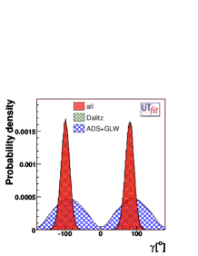
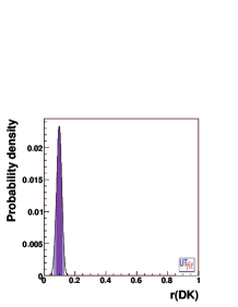
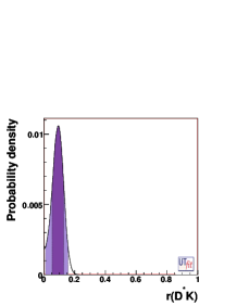
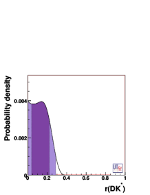
Figure 2: Probability density functions for $\phi_{3}/\gamma$ (top left), and $r_{B}$ in $B^{\pm}\rightarrow DK^{\pm}$ (top right), $B^{\pm}\rightarrow D^{*}K^{\pm}$ (bottom left), and $B^{\pm}\rightarrow DK^{*\pm}$ (bottom right) based on all available $\phi_{3}/\gamma$ measurements.

As it can be seen from Fig. 2 (top left), the $\phi_{3}/\gamma$ precision is mainly dominated by Dalitz analyses. These analyses have currently a hard-to-control uncertainty due to $D^{0}$ decay amplitude description, which is estimated to be 5–10^∘. At the current level of statistical precision this error starts to influence the total $\phi_{3}/\gamma$ uncertainty. A solution to this problem can be the use of quantum-correlated $D\overline{D}$ decays at $\psi(3770)$ resonance available currently at CLEO-c experiment, where the missing information about the strong phase in $D^{0}$ decay can be obtained experimentally modind ; modind2 . With CLEO-c data sample, the $\gamma$ uncertainty due to $D$ decay amplitude can be as low as $5^{\circ}$ (and, since it becomes a statistical uncertainty, it is more reliable than the current estimation based on the arbitrary variations of the model), while with the future BES-III sample it can be lowered to a degree level.

UTfit constraints on the Unitarity Triangle vertex are shown in Fig. 3. The plot shows a good agreement between the different measurements, and $\phi_{3}/\gamma$ results, although still have poorer sensitivity compared to other angles measurements, fit well into the whole picture.

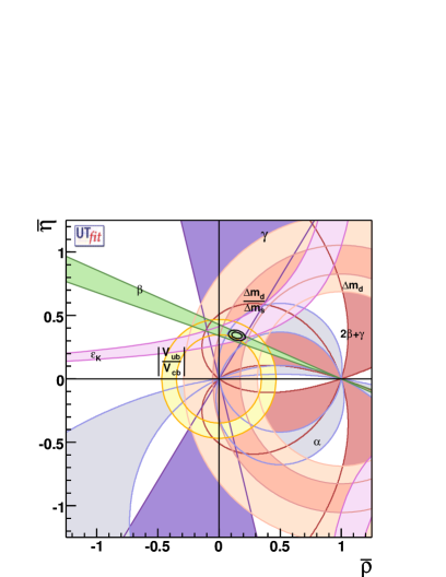
Figure 3: UTfit constraints on the Unitarity Triangle vertex including the latest $\phi_{3}/\gamma$ measurements.

VII Conclusion

In the past year, many new measurements related to a determination of $\phi_{3}/\gamma$ have appeared. As a result, strong evidence of a direct $CP$ violation in $B^{\pm}\rightarrow DK^{\pm}$ decays is obtained for the first time in a combination of B-factories results. Essential is that the amplitude ratio $r_{B}$, which determines the magnitude of the $CP$ violation and the precision of the $\phi_{3}/\gamma$ measurement, is finally constrained to be non-zero ($r_{B}=0.10\pm 0.02$ in the UTfit world average). This allows one to confidently extrapolate the sensitivity of $\phi_{3}/\gamma$ measurements to future experiments. Current world average is $\phi_{3}/\gamma=(81\pm 13)^{\circ}$; this value is dominated by the measurements based on Dalitz plot analyses of $D$ decay from $B^{\pm}\rightarrow D^{(*)}K^{(*)\pm}$ precesses. Although these analyses currently include a hard-to-control uncertainty due to the $D$ decay model, there are ways of dealing with this problem using charm data samples from CLEO-c and BES-III facilities, that should allow for a degree-level precision of $\phi_{3}/\gamma$ to be reached at the next generation $B$ factories.

References

- (1) BaBar Collaboration, B. Aubert et al., Phys. Rev. D 71, 032005 (2005).
- (2) Belle Collaboration, R. Itoh, Y. Onuki et al., Phys. Rev. Lett. 95 091601 (2005).
- (3) M. Gronau, D. London, D. Wyler, Phys. Lett. B 253, 483 (1991); M. Gronau, D. London, D. Wyler, Phys. Lett. B 265, 172 (1991).
- (4) BaBar collaboration, B. Aubert et al., Nucl. Instrum. Meth. A 479, 1 (2002).
- (5) Belle collaboration, A. Abashian et al., Nucl. Instrum. Meth. A 479, 117 (2002).
- (6) BaBar collaboration, B. Aubert et al., Phys. Rev. D 77, 111102 (2008).
- (7) D. Atwood, I. Dunietz, A. Soni, Phys. Rev. Lett. 78, 3357 (1997).
- (8) Belle collaboration, Y. Horii et al., Phys. Rev. D 78, 071901 (2008).
- (9) CLEO collaboration, D. M. Asner et al., Phys. Rev. D 78, 012001 (2008).
- (10) A. Giri, Yu. Grossman, A. Soffer, J. Zupan, Phys. Rev. D 68, 054018 (2003).
- (11) A. Bondar. Proceedings of BINP Special Meeting on Dalitz Analysis, 24-26 Sep. 2002, unpublished.
- (12) Belle Collaboration, A. Poluektov et al., Phys. Rev. D 73, 112009 (2006).
- (13) Belle collaboration, K. Abe et al., arXiv:0803.3375
- (14) BaBar collaboration, B. Aubert et al., Phys. Rev. D 78, 034023 (2008).
- (15) BaBar collaboration, B. Aubert et al., arXiv:0805.2001
- (16) BaBar collaboration, B. Aubert et al., Phys. Rev. D 71, 112003 (2005).
- (17) Belle collaboration, T. Gershon et al., Phys. Lett. B 624, 11 (2005).
- (18) R. Aleksan, T.C. Petersen, A. Soffer, Phys. Rev. D 67, 096002 (2003).
- (19) F. Polci, M.-H. Schune, A. Stocchi, arXiv:hep-ph/0605129
- (20) BaBar collaboration, B. Aubert et al., Phys. Rev. D77, 071102 (2008).
- (21) http://www.utfit.org
- (22) A. Bondar and A. Poluektov, Eur. Phys. J. C 47, 347 (2006).
- (23) A. Bondar and A. Poluektov, Eur. Phys. J. C 55, 51 (2008).