Adaptive tests of homogeneity for a Poisson process
Abstract
We propose to test the homogeneity of a Poisson process observed on a finite interval. In this framework, we first provide lower bounds for the uniform separation rates in norm over classical Besov bodies and weak Besov bodies. Surprisingly, the obtained lower bounds over weak Besov bodies coincide with the minimax estimation rates over such classes. Then we construct non asymptotic and nonparametric testing procedures that are adaptive in the sense that they achieve, up to a possible logarithmic factor, the optimal uniform separation rates over various Besov bodies simultaneously. These procedures are based on model selection and thresholding methods. We finally complete our theoretical study with a Monte Carlo evaluation of the power of our tests under various alternatives.
Mathematics Subject Classification: Primary: 62G10, Secondary: 62G20.
Keywords: Poisson process, adaptive hypotheses testing, uniform separation rate, minimax separation rate, model selection, thresholding rule.
1 Introduction
Poisson processes have been used for many years to model a great variety of situations: machine breakdowns, phone calls… Recently Poisson processes become popular for modeling occurrences of words or motifs on the DNA sequence (see Robin, Rodolphe and Schbath [24]). In this context, it is particularly important to be able to detect abnormal behaviors.
With such applications in mind, we consider in this paper the question of testing the homogeneity of a Poisson process . Since we can only observe a finite number of points of the process, this question has a sense only on a finite interval. For the sake of simplicity, we assume that the Poisson process is observed on the fixed set , and that it has an intensity with respect to some measure on with .
Denoting by the set of constant functions on , our aim is consequently to test the null hypothesis "", against the alternative "".
This problem of testing the homogeneity of a Poisson process has been widely investigated both from a theoretical and practical point of view (see Bain, Engelhardt, and Wright [2] or Cohen and Sackrowitz [7] for a survey and Bhattacharjee, Deshpande, and Naik-Nimbalkar [5] for a more recent work). In these papers, the alternative intensities are monotonous. Another related topic is the problem of testing the simple hypothesis that a stationary process is a Poisson process with a given intensity. We can cite for instance the papers by Fazli and Kutoyants [12] where the alternative is also a Poisson process with a known intensity, Fazli [11] where the alternatives are Poisson processes with one-sided parametric intensities, or Dachian and Kutoyants [10], where the alternatives are self-exciting point processes. The paper by Ingster and Kutoyants [18] is the closest one to the present work. The alternatives considered by Ingster and Kutoyants are Poisson processes with nonparametric intensities in a Sobolev or Besov ball with and known smoothness parameter .
However, in some practical cases like the study of occurrences of words or motifs on a DNA sequence, such smooth alternatives cannot be considered. The intensity of the Poisson process in these cases may burst at a particular position of special interest for the biologist (see Gusto and Schbath [14] for more details). The question of testing the homogeneity of a Poisson process then becomes "how can we distinguish a Poisson process with constant intensity from a Poisson process whose intensity has some small localized spikes?". This question has already been partially considered in the seventies in a precursory work by Watson [27]: he proposed a test based on the estimation of the Fourier coefficients of the intensity without evaluating the power of the resulting procedure.
In this paper, we focus on constructing adaptive testing procedures i.e. which do not use any prior information about the smoothness of the intensity , but which however have the best possible performances (in a minimax sense).
From a theoretical point of view, we evaluate the performances of the tests in terms of uniform separation rates with respect to some prescribed distance over various classes of functions. Given , a class of functions , and a level test with values in (rejecting when ), the uniform separation rate of over the class is defined as the smallest positive number such that the test has an error of second kind at most equal to for all alternatives in at an distance from . More precisely, if denotes the distribution of the Poisson process with intensity ,
| (1.1) | |||||
| (1.2) |
In view of the practical situations of our interest, we study some classes of alternatives that can be very irregular, for instance that can have some localized spikes. We then consider some classical Besov bodies and also some spaces that can be viewed as weak versions of these classical Besov bodies and that are defined precisely in the following. The interested reader may find in Rivoirard [23] some illustrations of functions in weak Besov spaces and how the smoothness parameters of the functions govern the proportion and amplitude of their spikes.
As a first step, we evaluate the best possible value of the uniform separation rate over these spaces. In other words, we give a lower bound for
| (1.3) |
where the infimum is taken over all level tests , and where can be either a Besov body or a weak Besov body. This quantity introduced by Baraud [3] as the -minimax rate of testing over or the minimax separation rate over is a stronger version of the (asymptotic) minimax rate of testing usually considered. The key reference for the computation of minimax rates of testing in various statistical models is the series of papers due to Ingster [16]. Concerning the Poisson model, Ingster and Kutoyants [18] give the minimax rate of testing for Sobolev or Besov balls with and smoothness parameter . They find that this rate of testing for the Sobolev or Besov norm or semi-norm is of order . Let us note that we find here lower bounds for the classical Besov bodies similar to Ingster and Kutoyants’ones. Furthermore, our lower bounds for the weak Besov bodies are larger than the ones for classical Besov bodies. Alternatives in weak Besov bodies are in fact so irregular that it is as difficult to detect them as to estimate them. The problem of estimation in weak Besov spaces is solved by using thresholding procedures: indeed the weak Besov spaces are closely related to the maxisets of those procedures (see Kerkyacharian and Picard [19] in the Gaussian framework and Reynaud-Bouret and Rivoirard [22] in a Poisson model). To our knowledge, no previous results of this kind exist for weak Besov bodies in testing problems, even in more classical statistical models, like the density model. Despite the similarity of both models, our lower bounds over weak Besov bodies cannot however be straightly transposed to the density model since our proofs heavily rely on the Poissonian independence properties.
As a second and main step, we construct non asymptotic level tests which achieve, up to a possible logarithmic factor, the minimax separation rates over many Besov bodies and weak Besov bodies simultaneously, whereas using no prior information about the smoothness of the intensity . Our idea here is to combine some model selection methods that are effective for alternatives in classical Besov bodies and a thresholding type approach, inspired by the thresholding rules used for adaptive estimation in weak Besov bodies. Key tools in the proofs of our results are exponential inequalities for U-statistics of order 2 due to Houdré and Reynaud-Bouret [15].
Of course, both model selection and thresholding approaches have already been used to construct adaptive tests in various statistical models. One can cite among others the papers by Spokoiny ([25] and [26]) in Gaussian white noise models or by Baraud, Huet and Laurent [4] in a Gaussian regression framework. These papers propose adaptive tests which combine methods closely related to both model selection and thresholding ones. As for the density framework, adaptive tests were proposed by Ingster [17] or Fromont and Laurent [13], using model selection type methods and by Butucea and Tribouley [6] using thresholding type methods.
The present work is organized as follows. In Section 2, we provide lower bounds for the uniform separation rates over various Besov bodies. Our testing procedures are defined in Section 3, and their uniform separation rates over Besov bodies are established in Section 4. We carry out a simulation study in Section 5 to illustrate these theoretical results, and the proofs are postponed to the last section.
2 Lower bounds for the minimax separation rates over Besov bodies
We consider the Poisson process with intensity with respect to some measure on , with . In the following, we assume that belongs to , and , and respectively denote the scalar product
the norm
and the associated distance.
Let us denote the Haar basis of by with
and
| (2.1) |
where .
We set and for every , .
We can now introduce the Besov bodies defined for , by
| (2.2) |
and more generally for , and ,
| (2.3) |
As in Reynaud-Bouret and Rivoirard [22], we also introduce some weaker versions of the above Besov bodies given for and by
| (2.4) |
Fixing some levels of error and in , and denoting by the set of functions bounded by , our purpose in this section is to find sharp lower bounds for , where is defined by (1.3).
Starting from a general idea developed by Ingster [16], we obtain the following result.
Theorem 1.
Assume that , , and , and fix some levels and in such that .
If , then
If , then
If and , then
Comments.
-
1.
For the whole set of parameters such that , we prove in Section 4 that these lower bounds are actually sharp.
-
2.
We have in case lower bounds which coincide with the minimax rates of testing obtained by Ingster and Kutoyants [18] when testing that a periodic Poisson process has a given intensity in the Besov spaces . We know (see Ingster [17] or Fromont and Laurent [13] for instance) that such rates can be achieved by some multiple testing procedure based on model selection type methods. This is the principle of our first procedure described in Section 3.1.
-
3.
We notice that the lower bounds obtained in case are equal to the minimax estimation rates on the maxisets of the thresholding estimation procedure, namely (see Kerkyacharian and Picard [19], Rivoirard [23], or Reynaud-Bouret and Rivoirard [22] for more details). This means that it is as difficult to test as to estimate over such classes of functions, phenomenon which is quite unusual. Since the minimax estimation rates on these classes are achieved by thresholding rules, it will be natural to construct a testing procedure based on thresholding methods: this is the idea that originated our second procedure described in Section 3.2.
3 Two tests of homogeneity
Let us recall that denotes the set of constant functions on and that we assume that belongs to .
In this section, we construct level tests of the null hypothesis "", against the alternative "", from the observation of the Poisson process , or the points of the Poisson process.
We introduce two testing procedures that come from two different statistical approaches. The first one originates in general model selection methods, while the second one is closer to the thresholding type methods.
In order to understand the global ideas of these procedures, let us notice that the squared distance between and the set of constant functions can be rewritten as
where , and for all , .
For every , can be estimated by
which is also equal to
From this variable, we deduce an unbiased estimator of given by :
| (3.1) |
Our first approach will consist in constructing estimators of based on a combination of the ’s, and in rejecting the null hypothesis when one of these estimators is too large. This was already the spirit of Watson’s procedure (see [27]). Our second approach is related to the test considered in Baraud et al. [4] to detect local alternatives. It will consist in considering a set of ’s and rejecting the null hypothesis directly when one of the ’s is too large. Let us now precisely define both procedures.
3.1 A first procedure based on model selection
Assuming that , a natural idea is to construct a testing procedure from an estimation of the squared distance .
In order to estimate this functional of , following the ideas of Laurent [20] and Fromont and Laurent [13], we introduce embedded finite dimensional linear subspaces of . We choose here to consider for the subspaces generated by the subsets of the Haar basis defined by (2.1), with . Each subspace is called a model. We denote by the dimension of , and by the orthogonal projection of onto the model .
Focusing on one model , we estimate by the unbiased estimator of given by
| (3.2) |
with defined by (3.1). The estimator obviously depends on the choice of the model .
Since we do not want to choose a priori such a model, we consider a collection of models where is a finite subset of , and the corresponding collection of estimators .
The procedure that we introduce here then consists in rejecting "" when there exists in such that the estimator given by (3.2) is too large.
At this point there are several ways to decide when is too large.
In all cases, we use the well-known argument that, conditionally on the event "the number of points falling into is ", the points of the process obeys the same law as a -sample with common density . It follows that for all ,
Under the null hypothesis, the intensity is constant on , and the ’s are i.i.d., with uniform distribution on . This distribution is free from the parameter . As a consequence, for every , we can introduce and estimate by Monte Carlo experiments the quantile of the distribution of under the null hypothesis, that we denote by .
We now consider the test statistics:
| (3.3) |
with to be correctly chosen.
Finally, we define the corresponding test function:
| (3.4) |
And our first test consists in rejecting the null
hypothesis when .
Let us see how we can choose so that our test has a level .
An obvious possibility is to set
This choice corresponds to a Bonferroni procedure and actually defines a level test. Indeed, for ,
Our choice for , inspired by Fromont and Laurent [13], leads to a less conservative procedure. It consists in setting
| (3.5) |
where is a collection of positive weights such that
For the same reason, we still obtain a level test and by definition, for every in .
3.2 A second procedure based on a thresholding approach
Let us recall here that the squared distance between and the set of constant functions is equal to and that defined by (3.1) is an unbiased estimator of . Based on general thresholding ideas, our second procedure consists in fixing some and rejecting the null hypothesis when there exists in such that is too large.
Let us now see what we mean by " is too large". We can still use the fact that
and that under the null hypothesis, the ’s are i.i.d., with uniform distribution on . We therefore introduce and estimate by Monte Carlo experiments the quantile of the distribution of under the null hypothesis, that we denote by . Notice that for , does not depend on .
We set
| (3.6) |
with to be correctly chosen.
We also define
| (3.7) |
Our test consists in rejecting the null
hypothesis when .
Let us now see how we choose . An obvious choice corresponding to the Bonferroni procedure would be
To obtain a less conservative procedure, we prefer setting
| (3.8) |
with
| (3.9) |
When ,
which means that defines a level test.
Note that .
Comments.
-
1.
Though the two testing procedures defined by (3.4) and (3.7) are very different by their spirit, they can formally be written in a common way. For any subset of , we denote by the subspace generated by , by the orthogonal projection of onto , and we introduce the unbiased estimator of . Then our test functions can be written as
(3.10) where
and is a finite collection of subsets of .
Noticing that , we can easily see that our first test amounts in taking a collection equal to , and . Furthermore, our second test amounts in taking a collection composed of all subsets of , and for , . Indeed, there exists a subset of such that if and only if there exists in such that .
Such a common expression will be particularly useful to derive the properties of the tests.
It also allows us to see our tests as multiple testing procedures. Indeed, we can consider that for each in , we construct a test rejecting the null hypothesis when . We thus obtain a collection of tests and we finally decide to reject the null hypothesis when it is rejected for at least one of the tests of the collection.
-
2.
Both procedures have a specific interest to prove the optimality of the lower bounds obtained in Theorem 1. We will actually prove in the next section that the first one achieves the lower bounds obtained in case of Theorem 1 (up to a possible logarithmic factor) whereas the second one achieves the lower bounds obtained in case of Theorem 1. However, if we want a procedure that achieves the lower bounds of cases and simultaneously, we will have to consider the test which consists in mixing the two procedures. In this case, we reject the null hypothesis when .
4 Uniform separation rates
In this section, we evaluate the performances of our new testing procedures from a theoretical point of view. More precisely, we prove that our procedures are optimal in the sense that their uniform separation rates over Besov bodies are of the same order as the lower bounds for obtained in Section 2. These results justify the construction of our procedures as well as they provide the upper bounds needed for the exact evaluation of the minimax separation rates over weak and classical Besov bodies in the Poisson framework.
In the following, the expression or is used to denote some constant which only depends on the parameters , and which may vary from line to line.
4.1 Uniform separation rates of the first procedure
4.1.1 The error of second kind
The aim of the following theorem is to give a condition on the alternative so that our first level test has a prescribed error of second kind.
Theorem 2.
Assume that , and that . Fix some levels and in , and let be the test function defined by (3.4). There exist some positive constants , , , and such that when satisfies
| (4.1) |
then
Comment. Considering here a multiple testing procedure instead of a simple one allows to obtain in the right hand side of the inequality an infimum over all in at the only price of introducing some terms in . These last terms will appear in the following uniform separation rates over classical Besov bodies as a factor, which is now known to be the price to pay for adaptivity in some classical statistical models. As a consequence, our multiple testing procedure is proved to be adaptive in Proposition 1 over classical Besov bodies, which would not occur with a simple testing procedure.
4.1.2 Uniform separation rates over Besov bodies
In this section, we evaluate the uniform separation rates where is defined by (1.1), and is any Besov body defined by .
Let us first notice that the functions of are well approximated by their projections onto subspaces of the collection considered in our first procedure, in the sense that if , then
As a consequence we can use Theorem 2 to obtain upper bounds for the uniform separation rates
of our test.
We denote by the integer part of .
Proposition 1.
Assume that . Given some levels and in , let defined by (3.4) with and for every in .
For every , there exists some positive constant such that when belongs to and satisfies
then
In particular, there exist some positive constants and such that if , then
Comments.
-
1.
Our first testing procedure is therefore adaptive: indeed, for large , it achieves the lower bounds for the minimax separation rates over all the spaces with simultaneously up to a possible factor (see Theorem 1).
However it does not achieve the optimal separation rates obtained in the case where . In this range of parameters, the regularity in is higher than the regularity in , meaning that the weak Besov body governs the separation rate. That is the reason why we introduced the thresholding type procedure. -
2.
The upper bound for the uniform separation rate obtained here is exactly of the same order as the (asymptotic) adaptive minimax rate of testing obtained by Ingster [17] in the density model, replacing the parameter of the Poisson model by the number of observations in the density model. In particular the factor is proved to be necessary in the density model for adaptive procedures.
-
3.
It is easy to see that when . So this result directly leads to upper bounds for the uniform separation rates of the test over the Besov bodies when . These rates, obtained in the Poisson framework, correspond to the ones in some Gaussian models (see Spokoiny [25] for instance) or in the density model (see Ingster [17]).
-
4.
Note that one could also consider some tests based on the Fourier basis as well as the Haar basis, as Fromont and Laurent [13] did in the density model. The theoretical results would remain unchanged, and the practical performances of the procedure would be better when considering smooth alternatives (see Fromont and Laurent [13] for more details and Section 5). We have only considered here tests based on the Haar basis for the sake of simplicity.
4.2 Uniform separation rates of the second procedure
4.2.1 The error of second kind
From the common expression (3.10) of the test function for the two procedures, we obtain here a result similar to Theorem 2 for the error of second kind of our second test.
Theorem 3.
Assume that , and that . Fix some levels and in , and let be the test function defined by (3.7). Recall that for any subset of , and respectively denote the subspace generated by and the orthogonal projection of onto . Denoting by the dimension of , there exist some positive constants , , , and such that when satisfies
| (4.2) |
then
4.2.2 Uniform separation rates over Besov bodies
Proposition 2.
Assume that . Given some levels and in , let be the test defined by (3.7) with .
For every and , there exists some positive constant such that if belongs to and satisfies
then
In particular, when , there exist some positive constants and such that if , then
Comments.
-
1.
Our second testing procedure is still adaptive: indeed, for large , it achieves the lower bounds for the minimax separation rates over all the spaces with simultaneously (see Theorem 1). In this case, we also remark that these rates are so large that there is no further price to pay for adaptivity in the sense that the upper bound does not involve any extra logarithmic factor. To our knowledge, this phenomenon is completely new for nonparametric testing procedures.
-
2.
Our second procedure achieves the lower bounds for the minimax separation rates over all the spaces with simultaneously, but it does not when . To obtain a test that achieves the minimax separation rates in both cases, our two procedures need to be combined.
4.3 Uniform separation rates of the combined procedure
Corollary 1.
Assume that . Fix some level and in . Let be the level test defined by (3.4) with and for every in . Let be the level test defined by (3.7) with . We consider .
For all and , there exist some positive constants and such that if , then
For all such that , there exist some positive constants and such that if , then
Comment. Since
the proof of this result directly comes from Proposition 1 and Proposition 2.
This final procedure actually matches the lower bounds of Theorem 1 and is consequently adaptive for the whole set of parameters such that (up to a factor when ). This also proves that the lower bounds of Theorem 1 are sharp for this set of parameters.
5 Simulation study
We aim in this section at studying the performances of our tests from a practical point of view. We consider several intensities defined on such that . denotes here a Poisson process with intensity on with respect to the Lebesgue measure, and the distribution of this process. We denote by the intensity which is constant (equal to 1) on . We choose and a level of test .
Let us now recall that our first procedure may be based on the test statistics
where denotes the quantile of under the hypothesis that , and is chosen such that :
The null hypothesis "" is rejected when .
We choose . For , we estimate the quantities
and the quantiles for all in .
These estimations are based on the simulation of independent samples with size , uniformly distributed on [0,1]. Half of the samples is used to estimate the
quantiles for varying on a grid over , and the other samples are used to estimate the probabilities occurring in the definition of . Finally, is estimated by the largest value on the grid such that these estimated probabilities are smaller than .
Let us also recall that our second procedure is based on the test statistics
where denotes the quantile of under the hypothesis that . For ,
with defined by (3.9).
The null hypothesis "" is rejected when .
We choose . For , we estimate the quantities
and the quantiles for all .
These estimations are based on the simulation of independent samples with size , uniformly distributed on [0,1]. Half of the samples is used to estimate the
quantiles for varying on a grid over , and the other samples are used to estimate the probabilities that occur in (3.9). Finally, we estimate in the same way as in the first procedure.
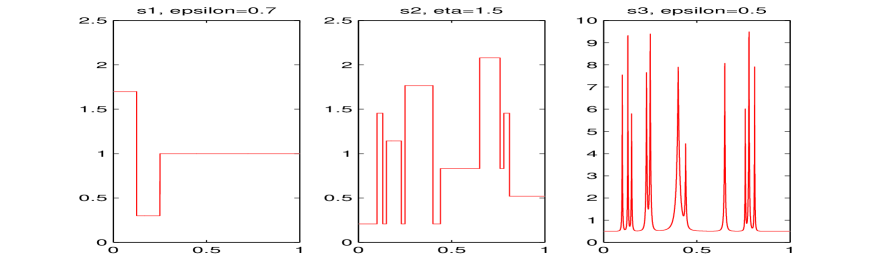
At this stage, we can estimate the powers of the two tests under various alternatives. The chosen alternatives are intensities that have already been studied among others by Reynaud-Bouret and Rivoirard [22], in the estimation problem. Since we are particularly interested in detecting the homogeneity of a Poisson process when the alternatives may be very irregular, we focus on the functions defined by:
where
, , and is such that .
These alternatives, for particular values of the parameters, are represented in Figure 1.
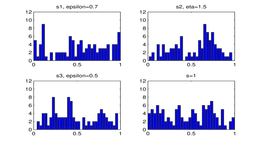
In Figure 2, we represent the histograms of one simulated sample for some of these alternatives and for a constant intensity on . Note that these histograms are clearly not sufficient to separate the alternatives from the null hypothesis.
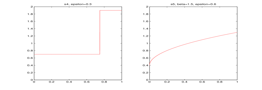
We also consider two monotonous alternatives defined by :
where , and .
These alternatives, for particular values of the parameters, are represented in Figure 3.
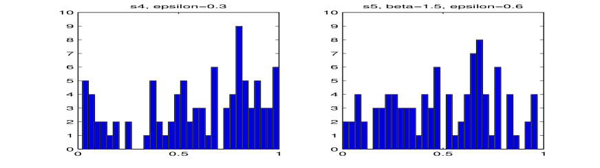
In Figure 4, we represent the histograms of one simulated sample for some of these alternatives.
For each alternative , we simulate Poisson processes with intensity on , and we estimate the powers of our two tests by :
and
where and are the test statistics and computed for the th simulated Poisson process.
We compare the obtained estimated powers with the estimated powers of the classical Kolmogorov and Smirnov’s test applied to the Poisson process conditionally on the event "the number of points of the Poisson process is ". The estimated powers of Kolmogorov and Smirnov’s test denoted by are also obtained by simulations of a Poisson process with intensity on .
The estimated powers are furthermore compared to the estimated powers of the tests studied in practice by the other authors. Such tests are in fact devoted to the particular case of increasing alternatives, which may be relevant in reliability contexts involving repairable systems. Bain, Engelhardt and Wright [2] and Cohen and Sackrowitz [7] consider in these contexts six well known tests. They show that two of these six tests, namely the so-called Laplace and tests (respectively studied first by Cox [8] and Crow [9]) are preferable to use.
The Laplace test is based on the statistics
where are the points of the process, and for every , is the quantile of the sum of independent random variables uniformly distributed on .
The test is based on the statistics
where for every , is the quantile of the chi square distribution with degrees of freedom.
Assuming that the intensity is increasing, the null hypothesis " is constant on " is rejected when or .
The readers need to be aware that these tests are especially constructed to detect homogeneity against increasing trend, when reading the estimated power tables.
Let us now present the results we obtained for the different tests. The estimated powers for Poisson processes with intensities , , , , and with various values of the parameters are given in the following tables.
Alternatives :
Alternatives :
Alternatives :
Alternatives :
Alternatives :
Comments.
-
1.
It first emerges from these results that when the alternatives are not increasing, our two tests have estimated powers significantly larger than the Laplace and tests that are designed for increasing alternatives, but also than Kolmogorov and Smirnov’s test. Furthermore, we can not give prior arguments to choose one of our two tests rather than the other one in these case. Indeed, we can notice that the first one is more powerful than the second one for alternatives which are rather smooth, but also for alternatives which are very irregular. Thus, in the case of non increasing alternatives such as , and , or in the practical situations of our interest such as the study of occurrences on DNA sequences where the intensities may have some localized spikes, this should argue in favor of the choice of our combined procedure.
-
2.
As for the increasing alternatives, the specific Laplace and tests remain as expected the most powerful ones, except for the alternatives , that are not as smooth as the alternatives. Kolmogorov and Smirnov’s test is also often more powerful than our tests. However, we know that in the case of smooth alternatives, we could probably significantly improve the estimated powers of our first test by using the Fourier basis instead of the Haar basis. Since our first test is very similar to Fromont and Laurent’s [13] one in the density model, we refer to this paper for more details. We could also consider a new test combining for instance our first test with the Laplace test.
6 Proofs
6.1 Proof of Theorem 1
Since it is easier to argue in terms of errors of second kind than in terms of minimax separation rates directly, we start by defining for all ,
where the infimum is taken over all level tests and by stating a useful and well-known lemma.
Lemma 1.
Let be a positive number, and , be subsets of .
If
then
If , then .
The proof of the lemma is straightforward.
Our aim here is to construct finite sets such that
| (6.1) |
and that
| (6.2) |
with as large as possible.
These finite sets are based on a family of functions such that for all , where is a function on such that
| (6.3) | |||
For , and , we introduce the set
| (6.4) |
As a first step, we notice that the functions ’s are positive as soon as and that for every , (see (6.1)).
As a second step, we want to find which positive leads to .
Let us recall a fundamental lemma which can be found in Ingster [16] or Baraud [3] for other frameworks.
Lemma 2.
Let be a probability measure on and let . Let be the distribution of a point process such that the conditional distribution of given that is a Poisson process with intensity . Let be the distribution of a Poisson process with constant intensity given by , and denote the expectation with respect to . Let be the likelihood ratio Then
Proof. The proof is obtained by rather straightforward computations. One has
where corresponds to the total variation norm. Hence,
But . So .
Regarding Lemma 2, we still have to find a distribution and such that which implies that
Let be a random vector, such that the ’s are i.i.d. Rademacher variables, taking the values and with probability . Let be a random vector, independent of and defined by , where is a set of indices drawn at random from without replacement.
Then the random function belongs to , which allows to take its distribution as .
Let us denote by the expectation with respect to the variable and by the expectation with respect to the random set defined above. By definition, Hence This can be rewritten as
where
Let be a random set of indices with the same distribution as and independent of . Then,
But under the distribution , the variables ’s are mutually independent since they only depend on the integrals of the Poisson process on intervals with disjoint support. Consequently,
| (6.5) |
We now need to compute and , and we use the following lemma.
Lemma 3.
Let be a function on . Then with the above notations,
Proof. When has the constant intensity , we know that conditionally on the event "the number of points falling into is ", the points of the process in obey the same law as a -sample with uniform distribution on . Then, one can easily see that
Under , has a Poisson distribution with parameter , therefore,
This concludes the proof.
From Lemma 3 and (6.1), one has that
Moreover,
Using Lemma 3 and (6.1) again, we finally obtain that
Hence, equation (6.5) gives
For fixed , is an hypergeometric variable with parameters . Hence, we know from Aldous [1] p. 173, that there exists a binomial variable with parameter such that . By Jensen’s inequality, we obtain that
Setting where the ’s are independent random Bernoulli variables with parameter , we easily obtain that
| (6.6) |
Following Baraud’s idea [3] and setting , since the function is increasing on , we have that if
then
Hence
and . As a conclusion, we obtain the following result, where the second part of the Proposition comes from a direct computation (see Baraud [3] for further details).
As a third step, we are now in position to find some (as large as possible) such that and that
.
Let us consider the set defined by (6.4) with , and .
Let , then can be rewritten as , with
Since , the condition ensures that
Let us define, for all ,
In order to ensure that belongs to , the function has to satisfy
Note that
Hence, we only need to have that
which is equivalent to
Moreover, if , then . Hence when , the condition
| (6.8) |
ensures that . From Proposition 3, we can conclude that when and , if
| (6.9) |
We now consider several cases, that are represented on the following figure.
In the following of this proof, will denote a positive constant that may depend on , and that may vary from one line to another.
Case 1. If , and , we set
and
We first check that for large enough since .
Then,
and
Finally, since
then
and
Case 2. If and , one chooses
and
We first check that for large enough since . Then,
and
Since moreover
and
Case 3. If , and , one chooses
and
With such a choice, one has that and
Furthermore
Hence,
when , and
when .
Case 4. If , one chooses with .
With such a choice,
and
Moreover
so
and
for large enough.
Case 5. If and , one takes
and
We first notice that . Then,
and
Moreover
Hence,
and
This concludes the proof of Theorem 1.
6.2 Proofs of Theorem 2 and Theorem 3
6.2.1 Preliminary results
We consider here the general test function , defined by (3.10), where
, and is a finite collection of subsets of . The collection and the quantile will be chosen to fit our two procedures respectively.
We begin to prove the following result.
Theorem 4.
Let , and fix and in . Assume that there exists some positive quantity such that
We recall that denotes the dimension of and we set .
There exist some positive constants and such that when satisfies
| (6.10) |
then
Proof. Let and in , and be a fixed intensity.
For every in , we can write in the following way :
By setting
and
we obtain the following decomposition :
Since , it follows that
Hence,
| (6.11) |
The aim of the following lemmas is to define positive quantities and , such that
Lemma 4.
There exists some positive constant such that for all and for all ,
Proof. Let us first notice that
Setting
| (6.13) |
we deduce from Theorem 4.2 in Houdré and Reynaud-Bouret [15] that there exists some absolute constant such that for all ,
where
Let us now evaluate , , and for every .
To give an upper bound for , we notice that
Since is an orthonormal basis on , one has
For , we use Cauchy-Schwarz inequality to see that
and
This implies that
Since is an orthonormal basis on , one has
As for , we can prove in the same way that
Moreover, for any fixed in ,
This implies that
Furthermore, for in [0,1],
Finally, , and this concludes the proof of Lemma 4.
By taking in Lemma 4, we obtain that a possible value for is
where is an absolute positive constant. We now use the following lemma, which derives from an analogue of Bennett’s inequality (see proposition 7 of Reynaud-Bouret [21], for instance).
Lemma 5.
There exists some positive constant such that for all ,
First note that
By using the elementary inequality , we obtain that
We deduce that there exists such that for all ,
By taking in Lemma 5, we obtain that a possible value for is
Replacing and in (6.12) by the possible values obtained above finally leads to the result of Theorem 4.
We now prove the following lemma that will provide an upper bound for the quantity occurring in Theorem 4.
Lemma 6.
Let be i.i.d. uniformly distributed on . For and , let
Let denote the dimension of and . There exists some absolute constant such that for all ,
| (6.14) |
Proof. If , hence (6.14) holds. Since for all , is orthonormal to , it follows that the variables are centered and we can apply Theorem 3.4 in Houdré and Reynaud-Bouret [15]. We now set We obtain that there exists some absolute constant such that for all ,
where
To evaluate , , , , we use arguments similar to the ones used in the proof of Lemma 4.
Since is an orthonormal basis on ,
Let and such that and . Then
By using Cauchy-Schwarz inequality, we obtain
One has for all , . As a consequence,
6.2.2 Proof of Theorem 2
Recall that the test function defined by (3.4) is of the same form as the test function (3.10) of Theorem 4 with , and , where denotes the quantile of . Since defined by (3.5) satisfies for all , one has that for all ,
In order to use Theorem 4, we then need to find some positive quantity such that
| (6.15) |
Let us first give an upper bound for for all in . We apply (6.14) with (note that ) and with . There exists some absolute constant such that
This allows us to obtain some such that (6.15) holds. It actually gives that
Now, from Bernstein’s inequality, we deduce that for all ,
Hence a possible value for is
6.2.3 Proof of Theorem 3
Recall here that the test function defined by (3.7) is of the same form as the test function (3.10) of Theorem 4 with , and , where denotes the quantile of conditionally on the event under the null hypothesis and defined by (3.9) satisfies for all .
Hence, we can prove Theorem 3 by using Theorem 4 and some positive quantity such that
Following the same lines of proof as in the previous section, let us first give an upper bound for .
Notice that is the quantile of the variable with . Since and , the inequality (6.14) implies that there exists some constant such that for all ,
Taking in this inequality leads to the conclusion that :
From Bernstein’s inequality, we deduce that a possible value for is
| (6.16) |
for some positive constant .
Since and , we obtain the result
of Theorem 3.
6.3 Proof of Proposition 1
We have already noticed that when belongs to , for all ,
Moreover, the constant can be replaced by , so we only need to find an upper bound for
Taking , with leads to , so
Since for all in , ,
We have that if and only if . Hence, we introduce
and we distinguish three cases.
When then belongs to and
When , this means that for all in , By taking , we obtain that
Finally, when , then for all in , , so by taking , we obtain that
This ends the proof.
6.4 Proof of Proposition 2
As in the proof of Proposition 1, the constant can be replaced by . Moreover, with the choice , we have that
and . So we only need to find an upper bound for
Let us introduce for all integer the subset of such that the elements of are the largest elements in .
We can notice that
On the one hand, since belongs to ,
On the other hand, since belongs to , then for all ,
Taking such that in the above inequality proves that all the coefficients of are smaller than and
Hence,
We have that if and only if . Hence, we introduce
and we distinguish two cases.
When , we clearly obtain that
On the one hand, when , this leads to
On the other hand, when , since , one has
Now, let us consider the case where . This means that for all such that , By taking , we obtain that
This concludes the proof of Proposition 2.
Acknowledgment. The authors acknowledge the support of the French Agence Nationale de la Recherche (ANR), under grant ATLAS (JCJC06137446) ”From Applications to Theory in Learning and Adaptive Statistics”.
References
- [1] Aldous, D.J. (1985) Exchangeability and related topics, Ecole d’été de probabilité de Saint-Flour XIII, Lect. Notes Math. 1117, 1-198.
- [2] Bain, L.J., Engelhardt, M., and Wright, F.T. (1985) Tests for an increasing trend in the intensity of a Poisson process: a power study, Journal of the Am. Statist. Assoc., 80, no. 390, 419-422.
- [3] Baraud, Y. (2002) Non asymptotic minimax rates of testing in signal detection, Bernoulli, 8, 577-606.
- [4] Baraud, Y., Huet, S., and Laurent, B. (2003) Adaptive tests of linear hypotheses by model selection, Ann. Statist., 31, no. 1, 225-251.
- [5] Bhattacharjee, M., Deshpande, J.V., and Naik-Nimbalkar, U.V. (2004) Unconditional tests of goodness of fit for the intensity of time-truncated nonhomogeneous Poisson processes, Technometrics, 46, no. 3, 330-338.
- [6] Butucea, C., and Tribouley, K. (2006) Nonparametric homogeneity tests, J. Statist. Plann. Inference, 136, 597-639.
- [7] Cohen, A., and Sackrowitz, H.B. (1993) Evaluating tests for increasing intensity of a Poisson process, Technometrics, 35, no. 4, 446-448.
- [8] Cox, D.R. (1955) Some statistical methods connected with series of events, Journal of the Royal Statist. Soc. Series B, 17, no. 2, 129-164.
- [9] Crow, L.H. (1974) Reliability and analysis for complex repairable systems, Reliability and Biometry, eds. F. Proschan and R. J. Serfling, Philadelphia: Society for Industrial and Applied Mathematics, 379-410.
- [10] Dachian, S., and Kutoyants, Yu.A. (2006) Hypotheses testing: Poisson versus self-exciting, Scand. J. Statist., 33, 391-408.
- [11] Fazli, Kh. (2007) Second-order efficient test for inhomogeneous Poisson processes, Statist. Inf. Stoch. Proc., 10, 181-208.
- [12] Fazli, Kh., and Kutoyants, Yu.A. (2005) Two simple hypotheses testing for Poisson process, Far East J. Theor. Stat., 15, no. 2, 251-290.
- [13] Fromont, M., and Laurent, B. (2006) Adaptive goodness-of-fit tests in a density model, Ann. Statist., 34, no. 2, 680-720.
- [14] Gusto, G., and Schbath, S. (2005) FADO : a statistical method to detect favored or avoided distances between motif occurrences using the Hawkes’ model. Statistical Application in Genetics and Molecular Biology, 4, no. 1, Article 24.
- [15] Houdré, C., and Reynaud-Bouret, P. (2003) Exponential inequalities, with constants, for U-statistics of order 2, Progr. Probab., Birkhauser, Basel, 56, 55-69.
- [16] Ingster, Yu.I. (1993) Asymptotically minimax testing for nonparametric alternatives I-II-III, Math. Methods Statist., 2, 85-114, 171-189, 249-268.
- [17] Ingster, Yu.I. (2000) Adaptive chi-square tests. J. Math. Sci., 99, no. 2, 1110-1119.
- [18] Ingster, Yu.I., and Kutoyants, Yu.A. (2007) Nonparametric hypothesis testing for intensity of the Poisson process, Math. Methods Statist., 16, no. 3, 217-245.
- [19] Kerkyacharian, G., and Picard, D. (2000) Thresholding algorithms, maxisets and well-concentrated bases, Test, 9, 283-344.
- [20] Laurent, B. (2005) Adaptive estimation of a quadratic functional of a density by model selection, ESAIM P& S, 9, 1-18.
- [21] Reynaud-Bouret, P. (2003) Adaptive estimation of the intensity of inhomogeneous Poisson processes via concentration inequalities, Probab. Theory Related Fields, 126, no. 1, 103-153.
- [22] Reynaud-Bouret, P., and Rivoirard, V. (2008) Near optimal thresholding estimation of a Poisson intensity on the real line, arXiv: 0810.5204.
- [23] Rivoirard, V. (2006) Nonlinear estimation over weak Besov spaces and minimax Bayes method, Bernoulli, 12, no. 4, 609-632.
- [24] Robin, S., Rodolphe, F., and Schbath, S. (2005) DNA words and models, Cambridge University Press.
- [25] Spokoiny, V. G. (1996) Adaptive hypothesis testing using wavelets, Ann. Statist., 24, no. 6, 2477-2498.
- [26] Spokoiny, V. G. (1998) Adaptive and spatially hypothesis testing of a nonparametric hypothesis, Math. Methods Statist., 7, no. 3, 245-273.
- [27] Watson, G.S. (1978) Estimating the intensity of a Poisson process, Applied time series analysis, 1st proceeding, Tulsa, 1976, 325-345.