Pair production in counter-propagating laser beams

Abstract

Based on an analysis of a specific electron trajectory in counter-propagating beams, Bell & Kirk (PRL 101, 200403 (2008)) recently suggested that laboratory lasers may shortly be able to produce significant numbers of electron-positron pairs. We confirm their results using an improved treatment of nonlinear Compton scattering in the laser beams. Implementing an algorithm that integrates classical electron trajectories, we then examine a wide range of laser pulse shapes and polarizations. We find that counter-propagating, linearly polarized beams, with either aligned or crossed orientation, are likely to initiate a pair avalanche at intensities of approximately $10^{24}\,\textrm{W\,cm}^{-2}$ per beam. The same result is found by modelling one of the beams as a wave reflected at the surface of an overdense solid.

1 Introduction

Within the next few years, powerful lasers may be able to realise intensities of $10^{23}$ to $10^{24}\,\textrm{W\,cm}^{-2}$ in the laboratory, enabling novel physical processes to be investigated [1, 2, 3]. One of these is the prolific production of electron-positron pairs predicted to occur when an electron is accelerated in counter-propagating laser beams [4].

Pair production has already been realised in the lab. using laser intensities $\sim 10^{20}\,\textrm{W\,cm}^{-2}$. The technique, proposed in [5], involves using the laser beams to accelerate electrons to MeV energies, and then allowing them to produce an electromagnetic cascade in a foil made of high-$Z$ target material. Depending on the experimental set-up, positrons are created either by the trident process, in which an energetic electron interacts with the electrostatic field of a target nucleus, or via an intermediate gamma-ray (produced by bremsstrahlung) that subsequently pair-creates in the field of a nucleus by the Bethe-Heitler process [6, 7, 8, 9]. The technique operates at relatively modest laser intensity, but converts only a small fraction of the laser pulse energy into pairs.

An alternative mechanism that has been intensively studied but not yet observed is the spontaneous creation of pairs out of the vacuum by laser beams. Schwinger [10] predicted spontaneous pair creation in an electric field that approaches the critical value $E_{\rm crit}=1.3\times 10^{18}\,\textrm{V\,m}^{-1}$, which is achieved at a laser intensity of roughly $10^{29}\,\textrm{W\,cm}^{-2}$. Conservation of energy and momentum forbids this process in a plane-wave beam, but it can operate in counter-propagating beams [11, 12] and may carry interesting information on the beam sub-structure [13]. The effect does not have a sharp threshold, but the rate drops rapidly as the amplitude $E$ of the electric field decreases, since it contains a factor $\textrm{exp}\left(-E_{\rm crit}/E\right)$. Detailed calculations predict observable consequences at intensities as low as $10^{26}\,\textrm{W\,cm}^{-2}$ [11], but these are unlikely to be achieved within the next few years.

A third mechanism of pair production using an intense laser beam was realised in an experiment at SLAC [14]. A beam of $46.6\,$GeV electrons was fired into a laser beam, where electron positron pairs were created. This was interpreted as being due to a two-step process: First a GeV photon was created by nonlinear Compton scattering of multiple laser photons by a relativistic electron. Then this photon interacted with multiple laser photons to create a pair. This technique is basically the same as the first method described above, except that the electrostatic field of the target nucleus is replaced by the electromagnetic field of the laser. The possibility that pairs might be directly produced by the trident process in the laser fields was not discussed. The positron yield observed in this experiment was very small.

The mechanism for prolific pair production suggested by [4] is closely related to that realised at SLAC. However, instead of using a particle accelerator, the laser beams themselves accelerate the relativistic electrons. The entire cycle of electron acceleration and pair creation (either by the electromagnetic analogue of the trident process or via an intermediate real photon) takes place when laser beams counter-propagate in an under-dense plasma. At intensities $\sim 10^{24}\,\textrm{W\,cm}^{-2}$ the number of pairs created per plasma electron was estimated by [4] to be about unity. Since each new electron and positron is, in its turn, accelerated in the laser beams, one expects an avalanche of pairs that should absorb a significant fraction of the laser pulse energy. This process would, therefore, swamp the pure vacuum effect.

The prediction of [4] was based on the analysis of a particularly simple electron orbit at the magnetic node in the field of two counter-propagating, circularly polarized pulses, and used simplified descriptions of the physical processes. In particular, the photon emissivity was treated using a monochromatic approximation. In this paper we examine this mechanism more closely. The analysis is extended in two ways: we use improved approximations to the physical processes, and embed these in a numerical scheme that follows the trajectory of an electron in more realistic models of the laser fields. Vacuum fields are used to describe the laser beams, which is appropriate if they propagate in an underdense plasma, and we examine the trajectories of initially nonrelativistic electrons picked up by the beams at different points in the plasma.

In section 2 we give details of the relevant physical processes. These all involve multi-photon interactions with the two laser beams. However, we show that, in the parameter range of interest, they can also be viewed as interactions of an electron or high-energy photon with uniform, static electromagnetic fields. The processes are (a) photon emission by a relativistic particle. In various special cases this is known as synchrotron radiation, magneto-bremsstrahlung, curvature radiation, non-linear Thomson scattering or non-linear Compton scattering; here we use the term “synchrotron radiation” to mean the generic process. We will assume the static field is incorporated exactly into the electron propagator, in which case the process is of first order in the fine-structure constant $\alpha_{\rm f}$. (b) The second-order (in $\alpha_{\rm f}$) process of pair production by a charged particle in a static field. (This involves an intermediate virtual photon and is the electromagnetic analogue of the trident process. In the following we simply refer to it as the “trident process”.) (c) The first-order process of pair production by a real photon (a synchrotron photon, for example) in the same static field.

In section 3 we describe our model of the laser fields, and give the classical equations of motion of the electron including radiation reaction. The way in which pair creation by the processes described in section 2 is implemented is discussed in section 3.3. Our results fall naturally into two parts. In section 4.1 we present calculations in counter-propagating, circularly polarized pulses with the same sense of rotation of the fields. The motivation here is to compare our results with [4] and to understand the influence of the improved treatment of the photon emissivity and of different choices of initial conditions of the electron trajectory. In section 4.2 we then examine pair production in more realistic pulses, with both circular and linear polarization. These pulses have a finite duration and the fields are assumed to be contained within a cylindrical region whose axis lies along the propagation direction. Our conclusions, which confirm and extend the predictions made in [4], are summarized in section 5.

2 Physical processes

2.1 The quasi-stationarity and weak-field approximations

For an electron in a monochromatic plane wave, the photon emissivity and pair-creation rate is a function of only two dimensionless, Lorentz invariant parameters [15]. These are the strength parameter of the wave

$$a = \frac{eE_{0}}{mc\omega_{\rm laser}}$$ (1)

where $E_{0}$ is the amplitude of the electric field and $\omega_{\rm laser}$ its angular frequency, and the parameter $\eta$ that determines the importance of strong-field quantum effects:

$$\eta = \frac{e\hbar}{m^{3}c^{4}}\left|F_{\mu\nu}p^{\nu}\right|$$ (2)

where $p^{\mu}$ is the four-momentum of the electron, $F^{\mu\nu}$ is the electromagnetic field tensor, and $\left|\dots\right|$ denotes the length of the four-vector. In terms of the field components $E_{i},B_{i}$ in Cartesian coordinates, with $i=1,\dots 3$:

$$F^{i0} = E_{i}\qquad F^{ij}\,=\,-\varepsilon_{ijk}B_{k}\qquad F^{\mu\nu}\,=\,-F^{\nu\mu}$$

and $\varepsilon_{ijk}$ is the antisymmetric Levi-Civita symbol.

The interaction of a particle with an arbitrary external electromagnetic field is more complex. However, two approximations simplify it considerably. The first is that of quasi-stationarity: “instantaneous” values of the transition rates are computed assuming the external field is constant in time, and these values are subsequently time-averaged. This requires that the variation timescale of the field is long compared to the coherence time associated with the interaction. In the monochromatic, plane-wave case, the coherence time is $t_{\rm coh}\approx\left(E_{\rm crit}/E_{0}\right)\left(\hbar/mc^{2}\right)$ [15]. Therefore, the variation timescale of the field is long compared to the coherence time of the interaction provided

$$a\gg 1$$ (3)

If this (Lorentz invariant) condition is satisfied, the instantaneous transition probabilities for an electron of given $p^{\mu}$ can be computed in the limit $a\rightarrow\infty$, i.e., for uniform, static fields. We assume that this argument can be generalized to the case of counter-propagating waves each of strength parameter $a$. A potential problem arises for those configurations where there exist points in space that are simultaneously nodes of both the electric and magnetic fields, since there the coherence length of the interaction becomes large. However, the processes that are important for pair production are confined to the regions of strong field, where the coherence length is short.

The situation can readily be visualized in the classical picture: the coherence length associated with the synchrotron radiation of a relativistic electron of Lorentz factor $\gamma$, is the path length over which the electron is deflected by an angle $1/\gamma$, which gives the same result as in the quantum case: $t_{\rm coh}\approx mc/\left(\left|e\right|E_{0}\right)$. Variations of the accelerating fields on lengthscales shorter than the deflection length occur only close to simultaneous nodes of the $\bm{E}$ and $\bm{B}$ fields. However, only relatively low frequency radiation is emitted in these regions.

The second approximation is that of weak fields. In an arbitrary, constant field, the transition probabilities may depend not only on $\eta$, but also on the two Lorentz invariant parameters associated with the field: $f=\left|E^{2}-B^{2}\right|/E_{\rm crit}^{2}$ and $g=\left|\bm{E}\cdot\bm{B}\right|/E_{\rm crit}^{2}$. Provided, however, that

$$f\ll 1\ \textrm{and}\ g\ll 1$$ (4)

and

$$\eta^{2}\gg\textrm{Max}(f,g)$$ (5)

one may neglect this dependence and evaluate the transition probabilities in any convenient field configuration that has the same value of the parameter $\eta$ [16, 15]. Analogously, pair production by a single high-energy photon in a laser field with $a\gg 1$ can be approximated as pair production in a uniform, static field, and the transition probability for interaction with the virtual photons of this field depends only on the parameter

$$\chi = \frac{e\hbar^{2}}{2m^{3}c^{4}}\left|F^{\mu\nu}k_{\nu}\right|$$ (6)

where $\hbar k^{\mu}=(\hbar\omega,\hbar\bm{k})$ is the photon four-momentum.

The situations we consider in this paper fulfil both the quasi-stationary requirement (3) and the weak-field conditions (4) and (5). At a laser wavelength of $\lambda_{\mu{\rm m}}\,\mu\textrm{m}$, the strength parameter in a single, linearly polarized beam of intensity $I_{24}\times 10^{24}\,\textrm{W\,cm}^{-2}$ is $a=855I_{24}^{1/2}\lambda_{\mu{\rm m}}$, so that the stationarity condition (3), is well satisfied in the range of interest ($\lambda_{\mu{\rm m}}=1$, $I_{24}=0.1\dots 1$). It is possible to configure laser beams in such a way as to reduce the variation timescale. For example, in a beam that is reflected from an overdense solid, high harmonics are generated [17, 18]. However, unless substantial power is present in harmonics numbers $n>100$, the stationarity approximation remains valid. The maximum field strength in a monochromatic, linearly polarized beam is $E/E_{\rm crit}=2.1\times 10^{-3}I_{24}^{1/2}$, and the field invariants $f$ and $g$ in (4) vanish in such a wave. In counter-propagating beams (each of intensity $I_{24}\times 10^{24}\,\textrm{W\,cm}^{-2}$), they do not vanish, but, although the field reaches twice the amplitude of the individual beams, one still has at all space-time points $f,g<1.6\times 10^{-5}I_{24}$, so that (4) is satisfied. Pair production becomes important for $\eta>0.1$, which requires relativistic electrons with $\gamma>50\,I_{24}^{-1/2}$. In this range, the weak field condition (5) is easily satisfied. Consequently, the transition probabilities for photon production and pair production by an electron (via a virtual photon) and by a real photon may be taken from computations performed for static, homogeneous magnetic fields that have the same value of the parameter $\eta$ or $\chi$, provided that this static configuration also fulfils the weak-field conditions.

In particular, choosing a situation in which an electron of Lorentz factor $\gamma$, or a photon of energy $\epsilon mc^{2}$, propagates normal to a constant, uniform magnetic field $B$, the relevant parameters are $\eta=\gamma B/B_{\rm crit}$ and $\chi=\left(\epsilon/2\right)B/B_{\rm crit}$. Since $f=\left(B/B_{\rm crit}\right)^{2}$, the weak-field condition (5) requires us to compute these transition probabilities for a field $B\ll B_{\rm crit}$, i.e., in the limit $\gamma,\epsilon\gg 1$. This case corresponds to the classical limit for the electron trajectory, where the particle energy is large compared to $\hbar eB/mc$, and to the case well above the threshold at $\epsilon=2$ for pair creation, in the case of the photon. These probabilities were calculated in the 1950’s; they are conveniently reviewed by Erber, [19], whose results we summarize in the following. Their application to arbitrary fields, as outlined above, and their generalization to particles of arbitrary spin is discussed by Baier & Katkov [16].

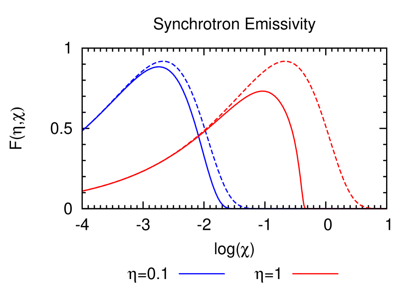
Figure 1: The quantum synchrotron function $F(\eta,\chi)$ as a function of the dimensionless photon frequency $\chi$ (see (6)). The parameter $\eta$, defined in (2), determines the importance of strong field QED effects; the energy of the radiated photon would equal that of the electron at $\log\chi=\log(\eta/2)$. The corresponding classical functions (see (9)) are shown as dashed lines.

2.2 Synchrotron radiation

The rate of production of photons by an electron of energy $\gamma mc^{2}$ moving normal to a magnetic field of strength $B=bB_{\rm crit}$ is defined as

$$\frac{\textrm{d}^{2}N}{\textrm{d}\chi\textrm{d}t} = \sqrt{3}\frac{mc^{2}}{h}\alpha_{\rm f}b\frac{F(\eta,\chi)}{\chi}$$ (7)

where $\chi$, defined in (6), describes the energy of the emitted photon. In this field configuration, $\eta=\gamma b$, and we can multiply this equation by $\gamma$ to display the Lorentz invariance of each side:

$$\gamma\frac{\textrm{d}^{2}N}{\textrm{d}\chi\textrm{d}t} = \sqrt{3}\frac{mc^{2}}{h}\alpha_{\rm f}\eta\frac{F(\eta,\chi)}{\chi}$$ (8)

For $\gamma\gg 1$ and $b\ll 1$, (i.e., under the weak-field conditions (4) and (5)) the function $F(\eta,\chi)$ is given in equation (2.5a) of [19], and is reproduced in our notation in A. In the classical limit, it becomes a function of $\eta$ and $\chi$ in the combination $\chi/\eta^{2}$:

$$F(\eta,\chi) \rightarrow f_{\rm synch}\left[4\chi/\left(3\eta^{2}\right)\right]\ \textrm{as}\ \hbar\rightarrow 0$$ (9)

where $f_{\rm synch}$ is the familiar expression for the synchrotron emissivity (summed over polarizations) in the Airy integral approximation [20]:

$$f_{\rm synch}(y) = y\int_{y}^{\infty}\,\textrm{d}t\,K_{5/3}(t)$$ (10)

The monochromatic approximation used in [4] is equivalent to the replacement

$$F(\eta,\chi) \rightarrow f_{\rm mono}\left[4\chi/\left(3\eta^{2}\right)\right]$$ (11)

with

$$f_{\rm mono}(y) = \frac{8\pi}{9\sqrt{3}}\delta\left(y-y_{0}\right)$$ (12)

together with the choice $y_{0}=0.29$ (which is where the function $f_{\rm synch}(y)$ has its maximum). The coefficients in front of the $\delta$-function in (12) ensure that the power radiated by an electron is the same in the classical and the monochromatic approximations.

In our problem, the most important difference between the quantum and classical emissivities is that the quantum emissivity is severely depleted for hard photons, when $\chi\sim\eta\sim 1$, and vanishes for photon energies larger than that of the incoming electron:

$$F(\eta,\chi) = 0\ \textrm{for}\ \chi\geq\eta/2$$ (13)

This has an important influence on pair production, since these photons subsequently have the highest probability of conversion. The effect is illustrated in figure 1. It is associated with a reduction in the (Lorentz invariant) total power $P$ radiated by the electron (integrated over all emitted photons):

$$P = \frac{2}{3}\alpha_{\rm f}\eta^{2}\,mc^{2}\frac{mc^{2}}{\hbar}g(\eta)$$ (14)

with

$$g(\eta) = \frac{3\sqrt{3}}{2\pi\eta^{2}}\int_{0}^{\infty}\,\textrm{d}\chi\,F(\eta,\chi)$$ (15)

The classical result is $g(\eta)=1$. For $\eta\ll 1$ the lowest order quantum correction gives [15]

$$g(\eta) \approx 1-\frac{55\sqrt{3}}{16}\eta$$ (16)

The full expression is given in A.

2.3 Trident pair production via virtual photons

Trident pair production via virtual photons is a second order process. The rate, computed using a Weizsäcker-Williams approximation, is presented by Erber [19]. This approximation involves treating the electromagnetic field of the incident electron as a superposition of virtual photons. The computation then essentially evaluates the dispersion relation for these photons in the magnetized vacuum. The imaginary part of the refractive index gives the absorption rate, i.e., the rate of pair production. This procedure should provide a reasonable approximation when the weak-field conditions are satisfied.

The rate of pair production for an electron of energy $\gamma mc^{2}$ moving normal to a constant magnetic field $B=bB_{\rm crit}$ is ([19], equation (4.4)):

$$\gamma\frac{\textrm{d}N_{\pm}}{\textrm{d}t} = 0.64\frac{mc^{2}}{h}\alpha_{\rm f}^{2}\eta\hat{\Omega}(\eta)$$ (17)

The function $\hat{\Omega}(\eta)$ is given in B. For small $\eta$ it can be approximated by

$$\hat{\Omega}(\eta) \approx \frac{\pi^{5/2}}{16}\left(3\eta\right)^{1/4}\textrm{exp}\left[-8/\left(3\eta\right)^{1/2}\right]$$ (18)

For $\eta\gg 1$, Erber gives the asymptotic value $\hat{\Omega}(\eta)\rightarrow\left(\pi^{2}/2\right)\ln\eta$.

2.4 Pair creation by synchrotron photons

The photon absorption coefficient in the ultra-relativistic limit required by the weak-field approximation is expressed by Erber [19] as an absorption probability per unit path length. Since we will be interested in the propagation of photons in electromagnetic fields that vary in space and time, we write the instantaneous absorption probability in terms of the differential optical depth $\textrm{d}\tau$ traversed by the photon in an interval of time $\textrm{d}t$ in the lab. frame:

$$\frac{\textrm{d}\tau}{\textrm{d}t} = \alpha_{\rm f}\frac{mc^{2}}{\hbar}\frac{mc^{2}}{h\nu}\chi T_{\pm}(\chi)$$ (19)

The function $T_{\pm}(\chi)$ is given approximately by

$$T_{\pm}(\chi) \approx 0.16\frac{K^{2}_{1/3}\left(\frac{2}{3\chi}\right)}{\chi}$$ (20)

For small $\chi$ it is proportional to $\textrm{exp}\left[2/\left(-3\chi\right)\right]$ and so is exponentially small, despite that fact that, in the weak-field approximation, the photon is always well above the kinematic threshold. The function peaks at $\chi\approx 8$ and falls off to higher $\chi$ as $\chi^{-1/3}$.

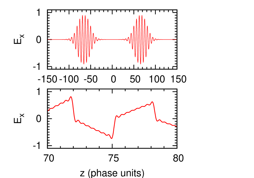
Figure 2: A snapshot of the electric field (normalized to unity at pulse centre) used to model laser pulses of finite duration according to (21), with $L=10\pi$ and $\Delta=10\pi/3$ (upper panel). At $t=0$ the leading edges of the pulses meet, the snapshot is taken at $t=-50$, corresponding to $26.5\,\textrm{fsec}$ before interaction for a laser wavelength of $1\,\mu\textrm{m}$. The lower panel shows the model waveform used for a reflected pulse, given by (22), with $n_{\rm max}=7$.

3 Trajectories

3.1 Laser fields

Bell & Kirk [4] considered a particle trajectory in counter-propagating monochromatic waves, with circular polarization, such that the field vectors rotate together at each point in space. This special case is considered in detail in Section 4.1. However, such an approach is limited in three respects:

1. Real laser pulses are of finite duration, the electrons they accelerate begin and end their trajectories outside of the pulse trains.

2. Circular polarization is a special case, that may not be the most favourable for pair production.

3. Monochromatic waves are an idealization. In particular, if one of the counter-propagating waves is produced by reflection from a solid surface, it will contain many high-order harmonics [17].

We lift these limitations by considering a range of laser waveforms as follows:

1. To model pulses of finite duration, we multiply the monochromatic wave by an envelope function $f(\phi)$ that contains two parameters: the duration or length $L$ of the pulses (in phase units) and the thickness $\Delta$ (also in phase units) of the pulse edges:

   $$f_{\pm}(\phi) = \frac{1}{4}\left[1\mp\tanh\left(\frac{\phi}{\Delta}\right)\right]\left[1\pm\tanh\left(\frac{\phi\pm L}{\Delta}\right)\right]$$ (21)

   Here $\phi=\phi_{\pm}=z\mp t$ is the phase of the wave, and the upper (lower) sign refers to the rightwards (leftwards) propagating pulse.

2. In order to avoid the stable $E=0$ nodes of the circularly polarized waves, we consider counter-propagating, linearly polarized waves with aligned polarization and with crossed polarization. In aligned polarization the electric fields of the counter-propagating beams are parallel, and in crossed polarization they are orthogonal.

3. The easiest way to produce counter-propagating waves may be to reflect a wave from a solid target. To account for the complex harmonic structure of the reflected wave [17, 18] we consider a leftward propagating wave with electric field:

   $$\bm{E} = \bm{\hat{x}}\frac{2}{\pi}\sqrt{\frac{\sqrt{3}}{2}}f\left(\phi_{-}\right)\left\{\sum_{n=0}^{n_{\rm max}}\frac{\sin\left[\left(2n+1\right)\phi_{-}\right]}{2n+1}-\frac{2\cos\left[\left(2n+1\right)\phi_{-}\right]}{\pi(2n+1)^{2}}\right\}$$ (22)

   This field is illustrated in figure 2. The Fourier series represents the summation of top-hat and saw-tooth functions. Terminating the expansion at $n=n_{\rm max}$ produces the high frequency ripple seen in the figure.

3.2 Equations of motion

The trajectory is treated classically: the electron is taken to be a point particle moving in prescribed external electromagnetic fields associated with the laser beam, and radiating energy continuously rather than in discrete jumps. When the electron becomes relativistic, radiation reaction plays an important role in the dynamics, and we incorporate it using the Landau-Lifshitz prescription [21]. To lowest order in $1/\gamma$, where $\gamma$ is the Lorentz factor, this leads to a force $\bm{f}_{\rm rad}$ that is anti-parallel to the particle momentum $\bm{p}$. Writing this in terms of the unit vector in the direction of the momentum, $\bm{p}=p\bm{\mu}$ one has:

$$\bm{f}_{\rm rad} = -\frac{2e^{4}}{3m^{4}c^{5}}\left|F_{\mu\nu}p^{\nu}\right|^{2}\bm{\mu}$$ (23)

$$= -\frac{2}{3}\alpha_{\rm f}\frac{m^{2}c^{3}}{\hbar}\eta^{2}\bm{\mu}$$ (24)

It can be shown [22] that the Landau-Lifshitz prescription for the classical radiation reaction force (the right-hand side of (24) does not contain $\hbar$, since $\alpha_{\rm f}\propto 1/\hbar$ and $\eta\propto\hbar$) is the lowest-order approximation in the small parameter $\eta\alpha_{\rm f}$ to the physically acceptable solution of the exact Lorentz-Abraham-Dirac equation. As such it is valid up to field strengths/energies much higher than those of interest here [23, 4]. The force corresponds exactly to the rate of transfer of momentum from the electron to the photon field according to the classical formula (9). However, the concept of a continuous classical trajectory fails at $\eta\approx 1$, where a single synchrotron photon takes off a significant fraction of the electron energy. Furthermore, quantum effects reduce the average power radiated, modifying it by the function $g(\eta)$ defined in (15) and plotted in figure 14. In this paper, we neglect the quantum fluctuations in the electron orbit, but take account of the reduction in radiated power by multiplying the radiation reaction force given in (24) by $g(\eta)$. The equations of motion for a particle of charge $q$, mass $m$ are then:

$$\beta\frac{\textrm{d}\bm{\mu}}{\textrm{d}t} = \frac{q}{\gamma mc}\left[\bm{E}_{\bot}+\beta\bm{\mu}\wedge\bm{B}\right]$$

$$\frac{1}{\gamma}\frac{\textrm{d}\gamma}{\textrm{d}t} = \left(\frac{q}{\gamma mc}\right)\beta\bm{\mu}\cdot\bm{E}-\frac{mc^{2}}{\hbar}\frac{2\alpha_{\rm f}\eta^{2}g(\eta)}{3\gamma}$$ (25)

where $c\beta=c\left(\gamma^{2}-1\right)^{1/2}/\gamma$ is the particle three speed, $\bm{E}_{\bot}$ is the component of $\bm{E}$ perpendicular to $\bm{\mu}$, and the radiation reaction term is given to lowest order in $1/\gamma$. Note that the parameter $\eta$ is determined by the component of the Lorentz force perpendicular to $\bm{\mu}$:

$$\eta = \frac{\gamma}{E_{\rm crit}}\left[\left(\bm{E}_{\bot}+\beta\bm{\mu}\wedge\bm{B}\right)^{2}+\left(\bm{\mu}\cdot\bm{E}\right)^{2}/\gamma^{2}\right]^{1/2}\,\approx\,\frac{\gamma\left|\bm{E}_{\bot}+\bm{\mu}\wedge\bm{B}\right|}{E_{\rm crit}}$$ (26)

Given $\bm{E}$ and $\bm{B}$ as functions of position and time, equations (25) are integrated forward in time using a standard fourth-order Runge-Kutta algorithm.

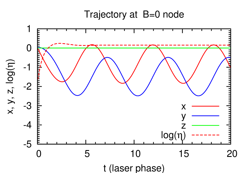
Figure 3: The trajectory of a particle initialized at a magnetic node in very long counter-propagating, circularly polarized pulses. Also plotted is the dependence of the parameter $\eta$ on time (measured in units of the laser phase).

3.3 Pair creation

In addition to the electron’s trajectory, we are interested also in the number and frequency of photons it radiates and, in particular, in the number of pairs created both by these photons as they propagate out through the laser beams and by direct trident pair production, according to (17).

The number of directly created, trident pairs is easily found by adding equation (17) to the set (25). This describes the monotonic growth in time of the number of pairs created by intermediate virtual photons $N_{\pm}(t)|_{\rm virtual}$.

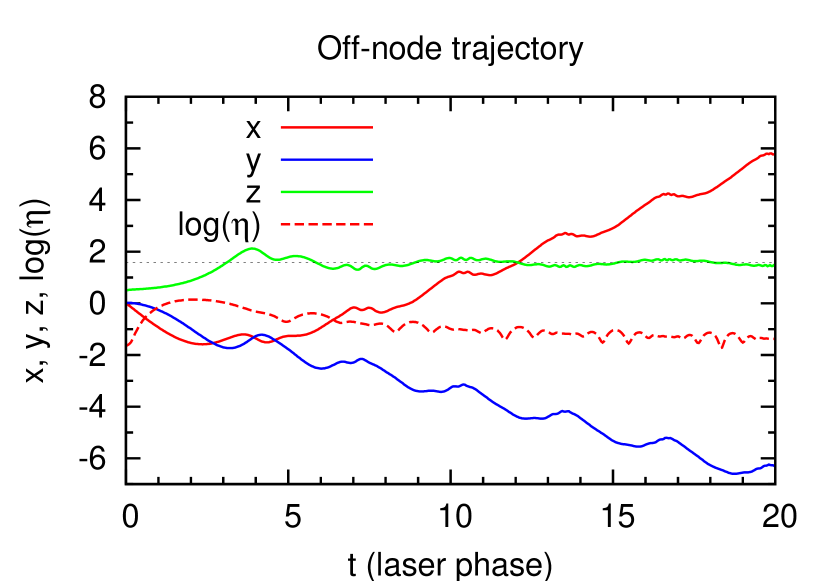
Figure 4: The trajectory of a particle initialized at $z=0.5$, between the nodes of the standing wave, in very long counter-propagating, circularly polarized pulses. The trajectory moves to a node of the electric field, located at $z=\pi/2$ (indicated by the dotted line). Also plotted is the dependence of the parameter $\eta$ on time (measured in units of the laser phase).

Pairs created by real photons are more difficult to compute. Suppose an electron emits a photon at time $t_{0}$, position $x_{0},y_{0},z_{0}$ with frequency $\nu$ (all measured in the lab. frame). The total optical depth to absorption for this photon is

$$\tau(\nu,t_{0},x_{0},y_{0},z_{0}) = \alpha_{\rm f}\frac{mc^{2}}{\hbar}\frac{mc^{2}}{h\nu}\int_{t_{0}}^{t_{\rm esc}}\textrm{d}t\,\chi(t)T_{\pm}[\chi(t)]$$ (27)

where the integration is along the photon’s ray path from emission to escape from the system at time $t_{\rm esc}$, and $T_{\pm}$ is defined in (20). In general, $\chi(t)$ depends on the photon’s frequency $\nu$ and its direction, which are constant along the ray path, as well as on the local electromagnetic field, which varies along this path. In analogy with (26), $\chi$ may also be defined as

$$\chi(t) = \frac{h\nu}{2mc^{2}}\frac{\left|\bm{E}_{\bot}+\hat{\bm{k}}\wedge\bm{B}\right|}{E_{\rm crit}}$$ (28)

where now $\bm{E}_{\bot}$ refers to the component of the electric field perpendicular to the propagation direction $\hat{\bm{k}}$ of the photon. Therefore, assuming the photon is emitted in the direction of motion of the electron, from (26) and (28) we can write the photon frequency in terms of its $\chi$-value at birth and the parameters $\gamma$ and $\eta$ of the parent electron at that instant:

$$\frac{h\nu}{2mc^{2}} \approx \frac{\chi\left(t_{0}\right)\gamma}{\eta}$$ (29)

The value of $\chi$ at any point on the ray path is then easily found from the local value of the electromagnetic fields, since both $\nu$ and $\hat{\bm{k}}$ are constant along this path. The total pair production probability per electron (via real photons) is then given by an integral of the pair production rate over the frequency of the emitted photons. The number of these pairs can also be described by a monotonically increasing function $N_{\pm}(t)|_{\rm real}$ of the time $t$ at which the pair-creating photons are emitted. This can be evaluated by adding another equation to the set (25):

$$\left.\frac{\textrm{d}N_{\pm}}{\textrm{d}t}\right|_{\rm real} = \int_{0}^{\eta/2}\textrm{d}\chi\,\frac{\textrm{d}N}{\textrm{d}\chi\textrm{d}t}\left[1-\textrm{exp}\left(-\tau\right)\right]$$ (30)

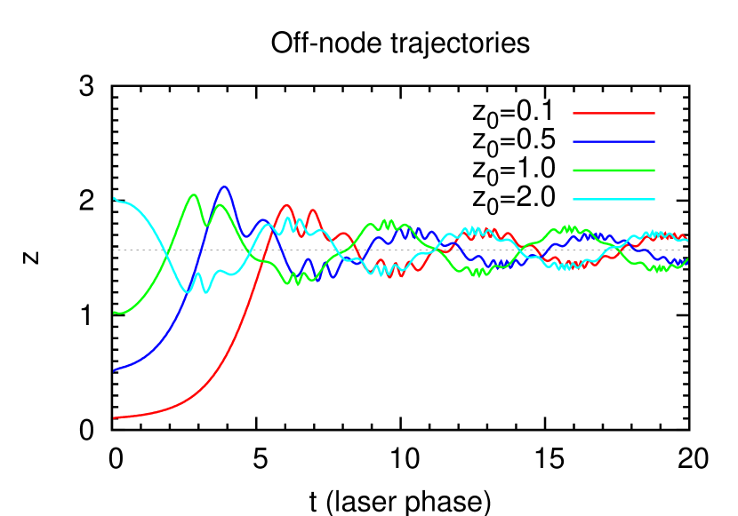
Figure 5: Trajectories of particles initialized at various positions in the standing wave in very long, counter-propagating, circularly polarized pulses. The $B=0$ node at $z=0$ appears to be unstable, whereas particles are attracted to the $E=0$ node at $z=\pi/2$.

Because the conversion probability, $1-\textrm{exp}(-\tau)$, depends on the photon’s path in the strong electromagnetic fields of the laser, a precise treatment requires a model of the spatial structure of the laser beams transverse to their direction of propagation. In this paper, we assume the pulses have cylindrical geometry. Taking the $z$-axis as the direction of propagation, the fields are assumed to be independent of $x$ and $y$ provided $x^{2}+y^{2}\leq R^{2}$, where $R$ is the radius of the cylinder, which we here set equal to one laser wavelength: $R=2\pi$, and to vanish outside this cylinder. In addition, we formally impose an upper limit on the length of the cylinder $\left|z\right|\leq z_{\rm max}$, although this is not relevant for the trajectories discussed in this paper. The cylindrical geometry of the pulses enters into the computations in two ways: particle trajectories are terminated when they leave the cylinder, and pair creation by photons is switched off when they leave the cylinder. We ignore diffraction effects by treating the wave as planar within the cylinder, but this will have little effect on the overall results. The main motivation for imposing the cylindrical boundary is to take approximate quantitative account of the escape of electrons and photons from the strong field regions in the intersecting beams.

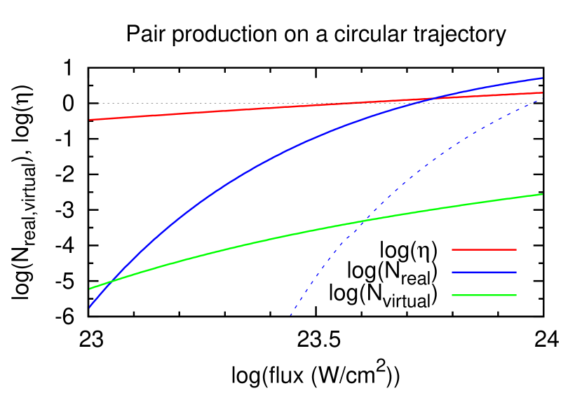
Figure 6: The number of pairs produced during a laser period by an electron following a circular trajectory at the magnetic node of the standing wave, as a function of the intensity of (one of) the counter-propagating, circularly polarized beams. Both the virtual and real photon channels are shown. In addition, the parameter $\eta$ defined in (2), which is constant on this trajectory, is shown. For comparison, the number of pairs predicted in [4] is shown as a dashed line.

This procedure should yield a realistic estimate of the number of pairs created by a single electron and the photons it radiates. However, in section 4.1, for the purpose of comparison we adopt an approximate method of computing the optical depth to absorption $\tau$ that is closely similar to the method used by Bell & Kirk [4]. The approximation consists of replacing the integral over the photon trajectory in (27) according to

$$\int_{t_{0}}^{\infty}\textrm{d}t\,\chi T_{\pm}(\chi) \rightarrow \frac{L_{\pm}}{c}\left<\chi\right>T_{\pm}\left(\left<\chi\right>\right)$$ (31)

The two parameters $\left<\chi\right>$ and $L_{\pm}$ can be interpreted as the effective value of $\chi$ averaged along the escaping ray path and the effective length of this path (assumed to be the same for each photon independent of its frequency or the position at which it is created).

As it propagates through the laser beams, the photon encounters electromagnetic fields that vary in both magnitude and direction. If, for example, the photon is emitted almost parallel to the local electric field, the initial value of $\chi$ is much lower than the average value it experiences on its escape path. To allow for this, we choose the average value $\left<\chi\right>$ so that it corresponds to a photon propagating perpendicular to an electric field whose strength equals the amplitude of the oscillating field at the point of emission. Formally, this involves summing the envelope functions ($f_{+}$ and $f_{-}$) introduced in (21):

$$\left<\chi\right>\left(\nu,t_{0},x_{0},y_{0},z_{0}\right)\,=\,$$ (32)

$$\frac{h\nu}{2mc^{2}}b\left[f_{+}(k_{\rm laser}z_{0}-\omega_{\rm laser}t_{0})+f_{-}(k_{\rm laser}z_{0}+\omega_{\rm laser}t_{0})\right]$$

so that, using (27) and (31), the approximate optical depth becomes

$$\left<\tau\right>\left(\nu,t_{0},x_{0},y_{0},z_{0}\right)\,=\,$$ (33)

$$\frac{L_{\pm}}{2}\alpha_{\rm f}\hbox{$a$}T_{\pm}\left(\left<\chi\right>\right)\left[f_{+}(k_{\rm laser}z_{0}-\omega_{\rm laser}t_{0})+f_{-}(k_{\rm laser}z_{0}+\omega_{\rm laser}t_{0})\right]$$

This quantity then replaces $\tau$ in (30). In [4], the effective path length was estimated to be one laser wavelength, so that we set $L_{\pm}=2\pi c/\omega_{\rm laser}$.

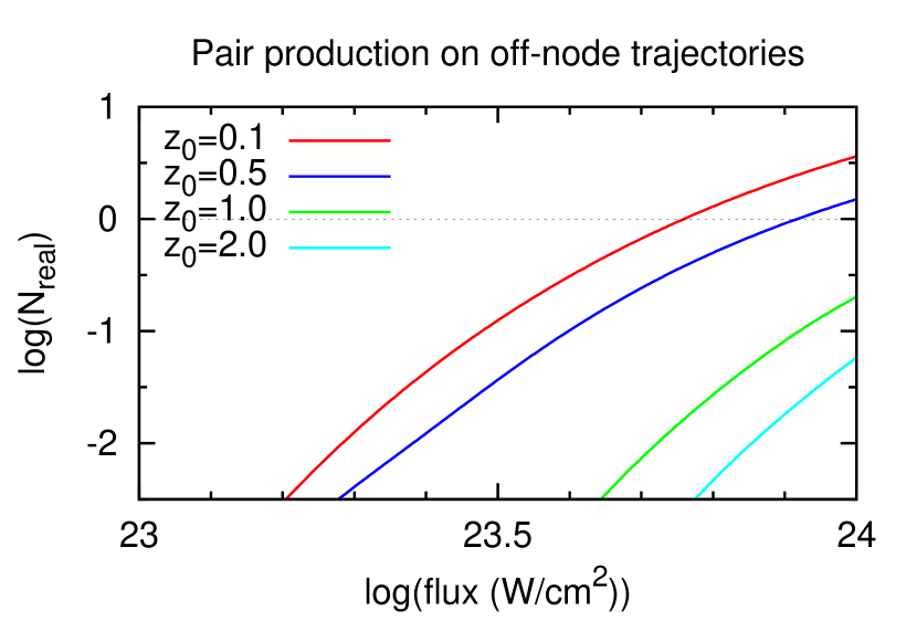
Figure 7: The number of pairs produced at $t=20$ (by which time this quantity has saturated) by an electron initialized at $t=0$ between the nodes of the standing wave, as a function of the intensity of (one of) the counter-propagating, circularly polarized beams. Only the real photon channel is shown. Initial conditions of the trajectories are as in figure 5

4 Results

Our results are divided into two parts. In the first, we consider counter-propagating, circularly polarized pulses of infinite duration. This enables us to compare with the results of [4]. Pair production in this case is treated using the approximation given in (31). In the second part, section 4.2, we consider a more realistic model, with pulses of finite duration. Pair production in this section is computed by integrating along the escape path of each photon at each timestep, and the laser fields are assumed to be confined to a cylindrical region.

4.1 Circularly polarized, long duration pulses

Bell & Kirk [4] analyzed a particularly simple trajectory: assuming two long pulses $L\rightarrow\infty$, they found that at the magnetic node ($B=0$), the particle settles into a circular orbit. This is illustrated in figure 3. The electron starts at $t=0$ at the origin, which is a node of the $B$ field, with velocity directed along the positive $y$ axis, and Lorentz factor $\gamma=10$. The intensity of a single laser pulse in this and the following examples is $6\times 10^{23}\,\textrm{W\,cm}^{-2}$. Within less than one hundredth of a laser period the particle turns to move in the negative $x$-direction, and, after a transient lasting less than one half of a laser period, the trajectory relaxes to a circle in the $x$-$y$ plane, with constant Lorentz factor $\gamma=760$.

Initializing an electron at a magnetic node is convenient for analytical calculations. However, it selects an electron trajectory that is particularly efficient at pair production. An electron initialized at rest at a node of the electric field, for example, remains at rest indefinitely. If a starting point in between the electric and magnetic nodes is chosen, the electron tends to drift towards the electric node, and lose energy in the process. This is illustrated in figure 4, which shows the trajectory of an electron initialized at $z=0.5$ (in units of $\lambda_{\rm laser}/2\pi$), with the same velocity as in figure 3. As well as a drift perpendicular to the laser beams towards positive $x$ and negative $y$, this trajectory starts to oscillate around the $E=0$ node at $z=\pi/2$, and slowly converges onto it. After a sharp rise associated with the rapid initial acceleration experienced by the electron, the parameter $\eta$, that controls pair production, decreases steadily with time.

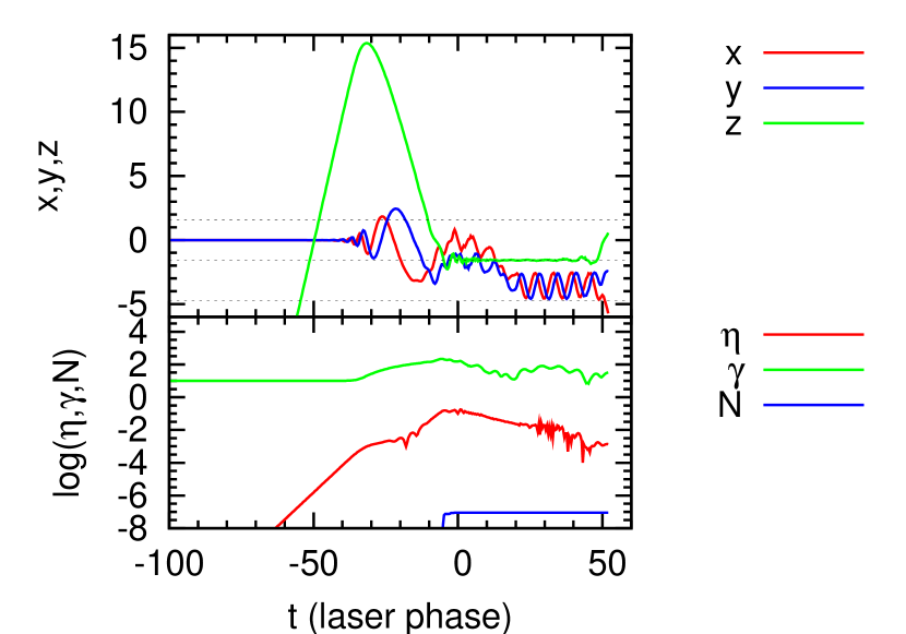
Figure 8: Sample trajectory in circularly polarized pulses of finite length, propagating along the $z$-axis. The upper panel shows position, the lower panel the Lorentz factor, the number $N$ of pairs produced per primary electron and the parameter $\eta$ defined in (2). When the pulses overlap the electric field vanishes at $z=(2n+1)\pi/2$, shown by dashed lines for $n=-2$, $-1$ and $0$.

Convergence on the $E=0$ node is a general property of the trajectories, as shown in figure 5. These examples demonstrate that the majority of the trajectories move swiftly to the vicinity of the $E=0$ mode, arriving in a zone around it of dimension less than one tenth of a wavelength within a single laser period. The subsequent motion is complex. As the electrons lose energy, their natural time and length scales decrease. After a long period close to such a node, this behaviour can place strong demands on the numerical integration method.

The number of pairs produced by a single electron following the trajectory illustrated in figure 3 for a range of laser intensities is shown in figure 6. The initial conditions were chosen to place the particle on the circular path analyzed in [4], thus avoiding short-lived transients. On such a trajectory, the parameter $\eta$ is constant. The number of pairs increases linearly with time, but, for comparison with [4], we select the value after one laser-period ($t=0$ to $t=2\pi$). This figure was computed using the approximate description of pair production described in section 3.3, with $L_{\pm}=2\pi c/\omega_{\rm laser}$. It is equivalent to the method used by Bell & Kirk [4] in their figure (1), in which, in addition, a monochromatic approximation to the synchrotron emission was adopted. As expected, allowing for the fact that even low energy electrons occasionally emit photons capable of pair producing leads to an increase in the number of pairs produced at low laser intensities. As a result, the pairs produced via virtual photons are overwhelmed by those produced by real photons, except at $I<10^{23}\,\textrm{W\,cm}^{-2}$, where the production rate is in any case very low. An additional factor contributing to the higher rate of pair production found in these calculations when compared to [4] is the inclusion of quantum corrections to the radiation reaction force via the factor $g(\eta)$ in (25). This leads to larger values of both $\gamma$ and $\eta$ for given laser intensity.

If the electron is initialized in between the nodes, pair production is reduced. This is shown in figure 7. In contrast with the circular trajectory at the $B=0$ node, the number of pairs produced when the particle is initialized off-node does not increase linearly with time, but saturates after a few laser periods. Consequently, figure 7 shows the time-asymptotic number of pairs, for the four initial conditions shown in figure 5.

The curve for $z_{0}=2.0$ demonstrates that, for circular polarization, electrons initialized close to the $E=0$ node move towards it rapidly without emitting as many pairs as those electrons initialized close to the $B=0$ node. Electrons with an unfavourable initial position do not contribute substantially to pair production. However, this negative effect is offset by the positive modifications illustrated in figure 6, The general conclusion of [4] that an ensemble of $N$ electrons produces approximately $N$ secondary pairs when the intensity of circularly polarized counter-propagating laser beams into which they are injected reaches $10^{24}\,\textrm{W\,cm}^{-2}$ remains unchanged.

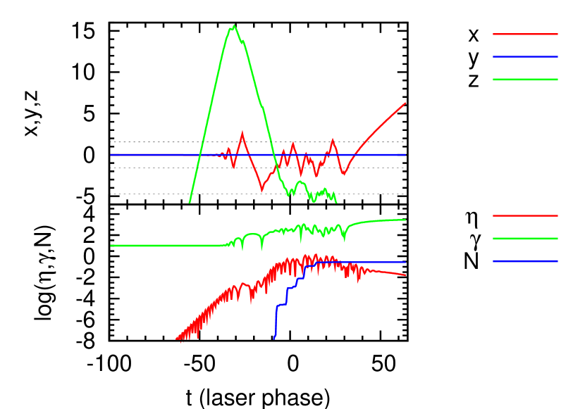
Figure 9: Sample trajectory in finite-length pulses with aligned, linear polarization.

4.2 Finite duration pulses in cylindrical geometry

The results of the previous section show that the position of a particle within a circularly polarized, long pulse train is important in determining the number of pairs it produces. In reality, however, pulse lengths are limited to a few laser wavelengths. As the pulses approach each other they pick up electrons and carry them forward on the front edge of the pulse until interaction starts. During interaction, the electron trajectory remains for an extended period at approximately constant $z$.

In the case of circular polarization, the particle stays close to a node of the electric field, but in the case of linear polarization, it samples a much larger region. In general terms, this is due to the characteristic figure-of-eight oscillation of an electron in a linearly polarized wave during which the electron oscillates in the direction parallel to beam propagation as well as in the perpendicular direction. In contrast, in a circularly polarized wave the electron can move smoothly, without parallel oscillation, towards the attracting $E=0$ node. This behaviour is illustrated in figures 8 and 9, in which the laser intensities and laser pulse shapes are the same but the polarizations differ. In each case, pulses of peak intensity $I_{24}=0.6$ with length $L=10\pi$ and thickness of the pulse edge $\Delta=10\pi/3$ were chosen. The trajectory was initialized at $t=-100$, when the pulses are well separated, at the position $x=y=0$, $z=-50$, moving in the positive $z$ direction with Lorentz factor $10$. The particle coasts at constant $\gamma$ until $t\approx-30$, when it encounters the leading edge of the leftward propagating wave. This wave picks it up, reversing its motion along $z$ and accelerating it until the pulses begin to interact at $t\approx 0$. In the circularly polarized case, the particle immediately drops onto the $E=0$ node at $z=-\pi/2$ (shown as a dashed line), the Lorentz factor falls and few pairs are created ($\sim 10^{-7}$ per primary particle). However, in the linearly polarized case, the particle performs substantial excursions in $z$, settling only briefly onto the $E=0$ node at $z=-3\pi/2$. During this time, the Lorentz factor fluctuates rapidly, with only a slight decrease in its average value. As a result, a relatively large number ($0.3$ per primary particle) of pairs are created. The trajectories terminate when the particle exits the cylinder containing the laser pulses at roughly $t=50$ for circular polarization and $t=65$ for linear polarization.

During the period when the pulses overlap, the electron trajectory is very complex, especially in the case of aligned linear polarisation. This makes it quite sensitive to the accuracy demanded of the integration algorithm, in the sense that a more stringent accuracy requirement leads to a trajectory that remains converged to larger times. For the trajectory shown in figure 9 we find that an error per step of less than $\delta=10^{-4}$ in position and in the angles (in radians) used to describe the unit vector $\bm{\mu}$ yields a converged trajectory up to $t=20$, whereas $\delta=10^{-6}$ extends this to $t=35$. (The example presented in figure 9 was computed with $\delta=10^{-8}$.) However, in both cases pair creation ceases well before accuracy is lost. We conclude that counter-propagating, circularly polarized beams are intrinsically inefficient at pair creation, at least when the fields rotate in the same direction, and do not consider them further.

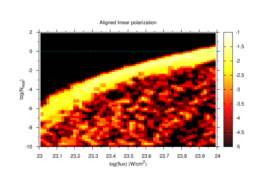
Figure 10: Pair production rates for a range of initial particle positions and for aligned linear polarization. Each pixel corresponds to a small range of laser intensity (“flux”, shown on the $x$-axis) and of the number $N_{\rm real}$ of pairs produced via the channel that involves an intermediate real photon (shown on the $y$-axis). The colour coding of a pixel indicates the logarithm (to base 10) of the probability that, given a flux in this interval, an electron with randomly chosen initial conditions (see text) will produce the corresponding number $N_{\rm real}$ of secondary pairs. Roughly $80\%$ of trajectories produce no pairs and so are not shown. At a laser flux of $10^{24}\,\textrm{W\,cm}^{-2}$, about $10\%$ of the particles reach the interaction region and the majority of these produce on average roughly one secondary pair.

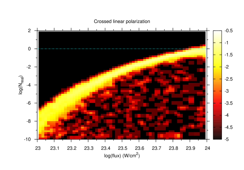
Figure 11: Pair production rates for a range of initial particle positions, as in figure 10, but for crossed linear polarization

Trajectories in linearly polarized pulses of finite length, contained in the cylindrical volume described above are sensitive to the point at which they are first picked up by a pulse, and to the time they subsequently spend at its leading edge, before they encounter the counter-propagating pulse. To take account of this, we present, in figures 10, 11 and 12, results obtained in pulses with $L=10\pi$ and $\Delta=10\pi/3$ by varying the initial $x$, $y$ and $z$ positions of the particle, whilst keeping the other initial conditions fixed. In each case, $3\times 10^{4}$ trajectories were computed, using randomly selected values of $x$ and $y$ uniformly distributed over the cross-section of the cylinder, random values of $z$ distributed uniformly over the range $-50$ to $0$, and random values of the pulse intensity, distributed uniformly in logarithm over the range $23<\log_{10}\left(I_{24}\right)<24$. The initial Lorentz factor is set to $10^{0.001}$, corresponding to an electron energy of about $1\,$keV, and the initial velocity is in the positive $z$-direction. In each of the three cases, roughly $80\,\%$ of the trajectories exit the cylinder before reaching the region where the laser beams interact, and so fail to produce pairs. The remaining trajectories were accumulated in 60 bins in intensity and 60 bins in pair yield, and are displayed as colour contour plots.

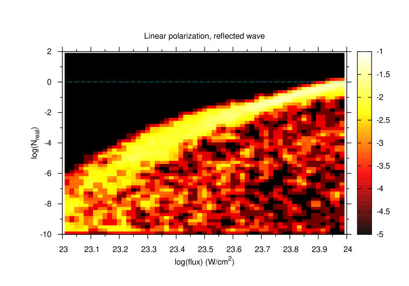
Figure 12: Pair production rates for a range of initial particle positions as in figure 10, but for aligned linear polarization with the leftward propagating wave modified to represent a reflected wave (with $n_{\rm max}=7$, see (22)).

The aim in figures 10, 11 and 12 is to test the sensitivity of pair production to polarization and pulse shape. In figure 11, “crossed polarization”, the electric field of one beam is in the $x$-direction whereas the field of the other beam is in the $y$-direction. In figures 10 and 12 the electric field of each pulse is in the $x$-direction. Figure 10 and 11 present results obtained using sinusoidal waves (modulated by the envelope function), whereas in figure 12 high harmonics are included in one of the waves, as illustrated in figure (2).

The possible advantage of the crossed configuration is that only at isolated points and times is the total electric field zero. When considering circular polarization in section 4.1, it was found that electrons congregated at the $E=0$ node and pair production was dramatically reduced. By eliminating the $E=0$ node this possibility is removed, which suggests that pair production might be increased. However, comparison of figures 10 and 11 shows that “aligned polarization” with both electric fields oscillating in the same direction performs nearly as well as crossed polarization –– possibly because the maximum electric field is larger by $\sqrt{2}$. In all three cases, (figures 10, 11 and 12) those trajectories that produce fewer than $10^{-10}$ pairs per primary electron are omitted. The remaining trajectories, show a large range in the number of pairs created, particuarly for aligned polarization at low laser intensity. However, most of the electrons sit on a band stretching from $N_{\rm real}\approx 10^{-8}$ at an intensity of $10^{23}\,\textrm{W\,cm}^{-2}$ to $N_{\rm real}\approx 1$ at $10^{24}\,\textrm{W\,cm}^{-2}$. This implies that pair production is effective for those particles that reach the interaction region, although only a minority of electrons do so if, as we assume here, they are injected uniformly over the beam cross-section just before the pulses meet.

In figure 12, the hypothesis is tested that pair production can be enhanced if the waveform contains high-frequency harmonics. At first sight, this is not implausible, because of the following argument: As discussed in [4], radiation losses prevent electrons reaching the Lorentz factor $\gamma_{\rm max}=eA_{\rm max}/mc^{2}$, where $A_{\rm max}$ is the maximum value of the electromagnetic vector potential. They do this by aligning the particle velocity and the accelerating force exerted by the field, and, therefore, not only reduce the Lorentz factor below $eA_{\rm max}/mc^{2}$, but also reduce the perpendicular component of the field and the parameter $\eta$ that controls both pair production and radiation losses. Prolific pair production would be much easier to achieve if radiation losses could be avoided whilst the electron is being accelerated. This suggests that if one of the counter-propagating waves contained abrupt changes in the electric or magnetic field it might be possible for the other wave to accelerate the electron in the direction of laser propagation to a high Lorentz factor but relatively small $\eta$. Subsequently, an abrupt change in the field direction caused by the first wave could lead to a large value of $\eta$ before radiation losses set in.

Such a situation might arise naturally when a sinusoidal wave is incident on a solid target since, as shown by [17], the reflected wave contains harmonics and abrupt changes in the electric field. According to PIC simulations [18], at an intensity of around $10^{21}\,\textrm{W\,cm}^{-2}$, the reflected waveform is generically similar to that in figure 2. The results presented in figure 12 are computed using this waveform for one of the waves while keeping the total intensity unchanged. However, at least in this example, our hypothesis is not confirmed: the presence of harmonics appears to make little difference and electrons produce roughly the same numbers of pairs as in sinusoidal waves with aligned linear polarization.

We conclude from figures 10, 11 and 12, that pair production is relatively insensitive to the orientation of the planes of linear polarization and to the waveform. While these results provide no indication that we can further increase pair production by a careful choice of waveform, they reinforce our general conclusion that strong pair production takes place whenever counter-propagating or reflected beams reach intensities around $10^{24}\,\textrm{W\,cm}^{-2}$.

5 Conclusions

In the above, we examine the possibility that an electron moving in counter-propagating laser beams of intensity $\sim 10^{24}\,\textrm{W\,cm}^{-2}$ could produce a substantial number of electron-positron pairs solely as a result of interaction with the laser fields. This is done using an accurate treatment of the physical processes, and embedding these in a numerical analysis of classical trajectories in realistic field configurations.

In the case of the photon production rate, we lift the monochromatic approximation used in [4] and take full account of quantum effects in the weak-field, quasi-stationary approximation (that is well-justified in the regime of interest). The result is shown in figure 6, where we examine a circular trajectory at the $B=0$ node of counter-propagating, monochromatic, circularly polarized beams and compare our results with [4]. Because even relatively low energy electrons produce a few hard photons that are subsequently capable of pair production, pairs start to appear at even lower intensities than previously predicted. The process of direct production via virtual intermediate photons, which was predicted to dominate over production via real photons for intensities less than $3\times 10^{23}\,\textrm{W\,cm}^{-2}$ is swamped by this effect for laser intensities exceeding $10^{23}\,\textrm{W\,cm}^{-2}$. At lower intensities, the virtual photon channel still dominates, but the overall rate of pair production is very small. At higher intensities, where the parameter $\eta$ is of the order of unity, classical synchrotron theory predicts the emission of photons whose energy exceeds that of the radiating electron. When this is corrected, (see figures 1 and 14), not only is the rate of emission of hard photons reduced, but the radiation reaction force acting on the electron is diminished. Radiation reaction significantly inhibits pair production on a circular trajectory, so that these two corrections have opposite effects on the pair production rate. Figure 6 shows that the overall effect is a slight enhancement of the pair production rate — we find the threshold above which an electron on this circular trajectory produces more than one pair per laser period is crossed at about $5\times 10^{23}\,\textrm{W\,cm}^{-2}$, compared to $10^{24}\,\textrm{W\,cm}^{-2}$ found in [4].

To take account of more realistic trajectories, we consider pulses of finite length and finite cross-section, with both linear and circular polarization, and inject electrons at a complete range of phases and positions. In addition to sinusoidal waveforms, we examine a laser pulse with harmonics, such as might be generated by reflection by an overdense plasma. The electron-laser interaction at the $B=0$ node considered in [4] is a special case, not least because the trajectory is unstable and the electrons migrate towards the $E=0$ node if the laser beams are circularly polarized. Nevertheless, under a wide range of laser pulse-shapes and polarizations with injection at random phases, we find that the conclusion is essentially unchanged: as the intensity of counter-propagating beams approaches $10^{24}\,\textrm{W\,cm}^{-2}$, the number of secondary pairs produced becomes roughly equal to the number of primary electrons interacting with the beams. Since each electron and positron so produced interacts further with the laser beams to produce further pairs, an avalanche of pair production is possible.

Further work is needed, particularly to remove the assumption that electron radiation losses are continuous, and to follow the interaction of primary and secondary particles with the complicated field structures produced by laser-solid interactions. However, our results strongly suggest that it may be possible to produce substantial pair plasmas with the next generation of extremely high-power lasers.

Appendix A Synchrotron emissivity

The function $F(\eta,\chi)$ is given in equations (2.5a…f) in [19]:

$$F(\eta,\chi) = \frac{8\chi^{2}}{3\sqrt{3}\pi\eta^{4}}\sum_{i=1}^{3}F_{i}(2\chi/\eta)\,J_{i}(y)$$ (34)

where

$$y = \frac{2\chi}{\left[3\eta\left(\eta-2\chi\right)\right]}$$ (35)

is the quantum equivalent of the classical parameter (photon frequency/characteristic synchrotron frequency). The $F_{i}$ are all positive, provided that the electron energy exceeds that of the photon, $\eta>2\chi$:

$$F_{1}(x) = 1+\left(1-x\right)^{-2}$$

$$F_{2}(x) = 2\left(1-x\right)^{-1}$$

$$F_{3}(x) = x^{2}\left(1-x\right)^{-2}$$ (36)

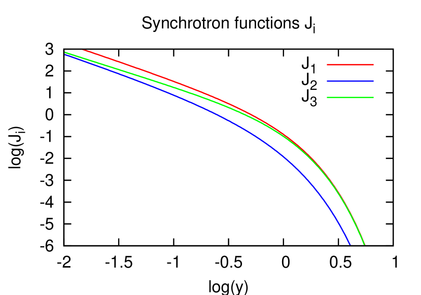
Figure 13: The synchrotron functions $J_{i}$ defined in (37)

The $J_{i}$ are also positive:

$$J_{1}(y) = \frac{1}{3y^{2}}\int_{y}^{\infty}\,\textrm{d}u\,\frac{u}{\sqrt{\left(u/y\right)^{2/3}-1}}K_{2/3}^{2}\left(u\right)$$

$$J_{2}(y) = \frac{1}{3y}\int_{y}^{\infty}\,\textrm{d}u\,\left(\frac{u}{y}\right)^{1/3}\sqrt{\left(u/y\right)^{2/3}-1}K_{1/3}^{2}\left(u\right)$$

$$J_{3}(y) = \frac{1}{3y^{2}}\int_{y}^{\infty}\,\textrm{d}u\,\frac{u}{\sqrt{\left(u/y\right)^{2/3}-1}}K_{1/3}^{2}\left(u\right)$$ (37)

For $y\ll 1$ they are well approximated by

$$J_{1}(y) \approx \frac{1}{3y^{5/3}}\int_{0}^{\infty}\,\textrm{d}u\,u^{2/3}K_{2/3}^{2}(u)$$ (38)

$$\approx 0.921y^{-5/3}$$

$$J_{2}(y) \approx \frac{1}{3y^{5/3}}\int_{0}^{\infty}\,\textrm{d}u\,u^{2/3}K_{1/3}^{2}(u)$$ (39)

$$\approx 0.307y^{-5/3}$$

$$J_{3}(y) \approx J_{2}(y)$$ (40)

These functions are plotted in figure 13

The function $g(\eta)$ defined in (15) that governs the total radiated energy can be written [24]:

$$g(\eta) = \frac{9\sqrt{3}}{8\pi}\int_{0}^{\infty}\,\textrm{d}y\,\left[\frac{2y^{2}K_{5/3}(y)}{\left(2+3\eta y\right)^{2}}+\frac{36\eta^{2}y^{3}K_{2/3}(y)}{\left(2+3\eta y\right)^{4}}\right]$$ (41)

This function is plotted in figure 14.

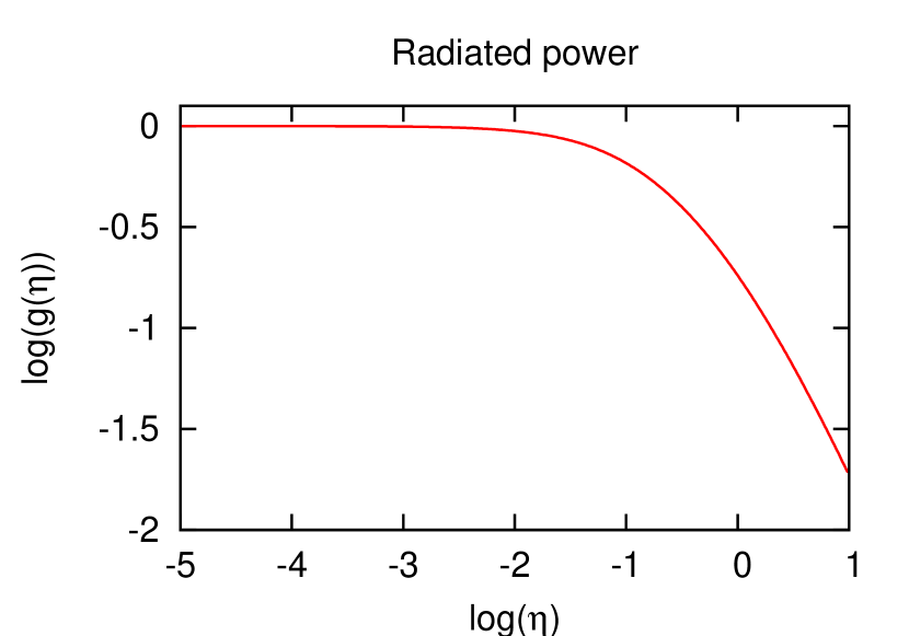
Figure 14: The function $g(\eta)$ defined in (15) that describes the quantum corrections to the total power in synchrotron radiation

A closely related alternative approximation to the synchrotron function is given by [25]:

$$F(\eta,\chi) = \frac{4\chi^{2}}{\eta^{2}}yK_{2/3}(y)+\left(1-\frac{2\chi}{\eta}\right)y\int_{y}^{\infty}\,\textrm{d}t\,K_{5/3}(t)$$ (42)

where $y$ is defined in (35).

Appendix B Pair-production via virtual photons

The function $\hat{\Omega}(\eta)$ can be evaluated starting from the expression given in [19] (equation A39):

$$\Omega^{\prime\prime}(x) = 4\pi\int_{0}^{\infty}\,\textrm{d}u\,K_{2}(4xu)K_{2/3}(1/u)$$ (43)

Mathematica gives an explicit expression for this integral in terms of the Meijer G function, and integrates it twice (using the boundary conditions $\Omega^{\prime}(\infty)=\Omega(\infty)=0$) to obtain

$$\hat{\Omega}(\eta) = \frac{\pi}{16}G^{6,0}_{2,6}\left(\frac{16}{9\eta^{2}}\!\!\!\!\!\!\!\!\!\!\!\!\!\!\!\!\begin{array}[]{ccc}&&\\ &&\\ &&\end{array}\right|\left.\begin{array}[]{cccccc}1,&3/2&&&&\\ &&&&&\\ 0,&0,&1/6,&1/2,&5/6,&2\end{array}\right)$$ (50)

References

References

- [1] J. Koga, T. Z. Esirkepov, and S. V. Bulanov. Nonlinear Thomson scattering with strong radiation damping. Journal of Plasma Physics, 72:1315–+, December 2006.
- [2] C. Müller, A. di Piazza, A. Shahbaz, T. J. Bürvenich, J. Evers, K. Z. Hatsagortsyan, and C. H. Keitel. High-energy, nuclear, and QED processes in strong laser fields. Laser Physics, 18:175–184, March 2008.
- [3] A. di Piazza and K. Z. Hatsagortsyan. Quantum interaction among intense laser beams in vacuum. European Physical Journal Special Topics, 160:147–155, July 2008.
- [4] A. R. Bell and J. G. Kirk. Possibility of Prolific Pair Production with High-Power Lasers. Physical Review Letters, 101(20):200403–+, November 2008.
- [5] J. W. Shearer, J. Garrison, J. Wong, and J. E. Swain. Pair Production by Relativistic Electrons from an Intense Laser Focus. Physical Review A, 8:1582–1588, September 1973.
- [6] E. P. Liang, S. C. Wilks, and M. Tabak. Pair Production by Ultraintense Lasers. Physical Review Letters, 81:4887–4890, November 1998.
- [7] T. E. Cowan, M. D. Perry, M. H. Key, T. R. Ditmire, S. P. Hatchett, E. A. Henry, J. D. Moody, M. J. Moran, D. M. Pennington, T. W. Phillips, T. C. Sangster, J. A. Sefcik, M. S. Singh, R. A. Snavery, M. A. Stoyer, S. C. Wilks, P. E. Young, Y. Takahashi, B. Dong, W. Fountain, T. Parnell, J. Johnson, A. W. Hunt, and T. Kühl. High energy electrons, nuclear phenomena and heating in petawatt laser-solid experiments. Laser Part. Beams, 17:773–783, October 1999.
- [8] K. Nakashima, T. E. Cowan, and H. Takabe. Electron-Positron Pair Production by Ultra-Intense Lasers. In K. Nakajima and M. Deguchi, editors, Science of Superstrong Field Interactions, volume 634 of American Institute of Physics Conference Series, pages 323–328, October 2002.
- [9] H. Chen, S. C. Wilks, J. D. Bonlie, E. P. Liang, J. Myatt, D. F. Price, D. D. Meyerhofer, and P. Beiersdorfer. Relativistic Positron Creation Using Ultraintense Short Pulse Lasers. Physical Review Letters, 102(10):105001–+, March 2009.
- [10] J. Schwinger. On Gauge Invariance and Vacuum Polarization. Physical Review, 82:664–679, June 1951.
- [11] S. S. Bulanov, N. B. Narozhny, V. D. Mur, and V. S. Popov. Electron-positron pair production by electromagnetic pulses. Soviet Journal of Experimental and Theoretical Physics, 102:9–+, January 2006.
- [12] M. Ruf, G. R. Mocken, C. Müller, K. Z. Hatsagortsyan, and C. H. Keitel. Pair production in laser fields oscillating in space and time. Physical Review Letters, 102:080402–+, 2009.
- [13] F. Hebenstreit, R. Alkofer, G. V. Dunne, and H. Gies. Momentum signatures for Schwinger pair production in short laser pulses with a sub-cycle structure. Physical Review Letters, 102:150404–+, 2009.
- [14] D. L. Burke, R. C. Field, G. Horton-Smith, J. E. Spencer, D. Walz, S. C. Berridge, W. M. Bugg, K. Shmakov, A. W. Weidemann, C. Bula, K. T. McDonald, E. J. Prebys, C. Bamber, S. J. Boege, T. Koffas, T. Kotseroglou, A. C. Melissinos, D. D. Meyerhofer, D. A. Reis, and W. Ragg. Positron Production in Multiphoton Light-by-Light Scattering. Physical Review Letters, 79:1626–1629, September 1997.
- [15] V. I. Ritus. Quantum effects in the interaction of elementary particles with an intense electromagnetic field. Moscow Izdatel Nauka AN SSR Fizicheskii Institut Trudy, 111:5–151, 1979.
- [16] V. N. Baǐer and V. M. Katkov. Processes Involved in the Motion of High Energy Particles in a Magnetic Field. Soviet Journal of Experimental and Theoretical Physics, 26:854–+, April 1968.
- [17] T. Baeva, S. Gordienko, and A. Pukhov. Theory of high-order harmonic generation in relativistic laser interaction with overdense plasma. Phys. Rev. E, 74(4):046404–+, October 2006.
- [18] T. Baeva. Coherent X-rays from relativistic plasmas. Annual report of the UK Central Laser Facility, pages 103 – 106, 2008.
- [19] T. Erber. High-Energy Electromagnetic Conversion Processes in Intense Magnetic Fields. Reviews of Modern Physics, 38:626–659, October 1966.
- [20] D. B. Melrose. Plasma Astrohysics. Nonthermal processes in diffuse magnetized plasmas - Vol.1: The emission, absorption and transfer of waves in plasmas; Vol.2: Astrophysical applications. New York: Gordon and Breach, 1980, 1980.
- [21] L. D. Landau and E. M. Lifshitz. The Classical Theory of Fields. Course of theoretical physics - Pergamon International Library of Science, Technology, Engineering and Social Studies, Oxford: Pergamon Press, 1975, 4th rev.engl.ed., 1975.
- [22] N. P. Klepikov. Methodological Notes: Radiation damping forces and radiation from charged particles. Soviet Physics Uspekhi, 28:506–520, June 1985.
- [23] A. di Piazza. Exact solution of the Landau-Lifshitz equation. Lett. Math. Phys., 83:305–313, 2008.
- [24] A. A. Sokolov and I. M. Ternov. Synchrotron Radiation. Berlin: Akademie-Verlag, 1968.
- [25] A. I. Akhiezer, N. P. Merenkov, and A. P. Rekalo. On a kinetic theory of electromagnetic showers in strong magnetic fields. Journal of Physics G Nuclear Physics, 20:1499–1514, September 1994.