The solar Ba ii  4554 Å  line as a Doppler diagnostic: NLTE analysis in 3D hydrodynamical model

Abstract

Aims. The aim of this paper is to analyse the validity of the Dopplergram and $\lambda$-meter techniques for the Doppler diagnostics of solar photospheric velocities using the Ba ii 4554 Å line.

Methods. Both techniques are evaluated by means of NLTE radiative transfer calculations of the Ba ii 4554 Å line in a three-dimensional hydrodynamical model of solar convection. We consider the cases of spatially unsmeared profiles and the profiles smeared to the resolution of ground-based observations.

Results. We find that: (i) Speckle-reconstructed Dopplergram velocities reproduce the “true” velocities well at heights around 300 km, except for intergranular lanes with strong downflows where the velocity can be overestimated. (ii) The $\lambda$-meter velocities give a good representation of the “true” velocities through the whole photosphere, both under the original and reduced spatial resolutions. The velocities derived from the inner wing of smeared Ba ii 4554 Å line profiles are more reliable than those for the outer wing. Only under high spatial resolution does the inner wing velocities calculated in intergranular regions give an underestimate (or even a sign reversal) compared with the model velocities. (iii) NLTE effects should be taken into account in modelling the Ba ii 4554 Å line profiles. Such effects are more pronounced in intergranular regions.

Conclusions. Our analysis supports the opinion that the Dopplergram technique applied to the Ba ii 4554 Å line is a valuable tool for the Doppler diagnostics of the middle photosphere around 300 km. The $\lambda$-meter technique applied to this line gives us a good opportunity to “trace” the non-thermal motions along the whole photosphere up to the temperature minimum and lower chromosphere.

1 Introduction

First studies of the barium lines in stellar spectra started in the 1930s. One of the examples of these earlier studies is by Bidelman & Keenan (1951), who pointed out that the anomalous strength of the Ba ii  4554 Å line in some stars could be explained by a deviation from local thermodynamic equilibrium (NLTE). At the present time stellar studies are aimed at the abundance determination of barium isotopes using one-dimensional (1D) plane–parallel atmospheric models and the NLTE assumption (Gigas, 1988; Mashonkina & Gehren, 2000; Mashonkina et al., 2003, 2008; Mashonkina & Zhao, 2006; Short & Hauschildt, 2006). Such studies play important role in estimating the yields of s- and r-processes in the nucleosynthesis of heavy elements in the Galaxy.

Barium lines in the solar spectrum have been studied since 1960s. Until the mid-seventies most the studies aimed at determining the solar barium abundance using a 1D$+$LTE approach (Goldberg, Müller, & Aller, 1960; Lambert & Warner, 1968; Holweger & Müller, 1974). The only exception was the publication of Tandberg-Hanssen (1964); Tandberg-Hanssen & Smythe (1970), who had shown the importance of NLTE effects for the formation of the Ba ii 4554 Å  line. Later, Rutten (1977, 1978); Rutten & Milkey (1979) tackled in detail the NLTE Ba ii line formation problem. Empirical analyses of centre-to-limb observations by Rutten (1978) have shown that the source function of the Ba ii 4554 Å  line deviates significantly from the Planck function. The effects of partially coherent scattering have also to be taken into account in order to reproduce observations away from the disc centre. The hyperfine structure and isotopic shift play a very important role in the analysis of this line as well.

For several reasons, a new debate has arisen in the recent literature on the solar Ba ii 4554 line. Firstly, a more realistic representation of the solar atmosphere by three-dimensional (3D) hydrodynamical simulations has become available. Relaxing the constraints of the plane–parallel (1D) modelling a new LTE abundance analysis by Asplund et al. (2005) resulted in a photospheric barium abundance of $A_{\rm Ba}=2.17$, close to the meteoritic value $A_{\rm Ba}=2.16$. While the recent NLTE analysis by Olshevsky et al. (2008) based on a 3D model lowers the value of $A_{\rm Ba}$ strictly to the meteoritic one. Note that the classical 1D-approach resulted in a rather wide spread of the solar barium abundance $A_{\rm Ba}=2.09$ (Ross & Aller, 1976), $A_{\rm Ba}=2.13$ (Grevesse, 1984), and $A_{\rm Ba}=2.40$ (Rutten, 1978).

Secondly, according to the atlas of the “Second Solar spectrum” (Gandorfer, 2002), the linear polarization $Q/I$ of this line close to the limb ($\mu=0.1$) is very strong ($0.6\%$). The recently published theoretical investigation on the role of resonance scattering and magnetic fields in the polarization signals of both Ba ii  4934 Å, and 4554 Å  resonance lines by Belluzzi et al. (2007) has demonstrated their importance for the measurements of weak magnetic fields on Sun and stars.

Finally, several properties of the Ba ii 4554 Å line have drawn attention to it as a diagnostic tool for the velocity field of the solar atmosphere. Due to the large atomic weight of barium (137.4 a.u.), one might expect low sensitivity of the line opacity to temperature variations and line-width insensitivity to thermal broadening. In addition, the Ba ii  4554 Å line has steep wings and a deep core. In a standard 1D model the core of this line is formed around 700 km in the chromosphere while the wings are photospheric (Olshevsky et al., 2008; Sütterlin et al., 2001). As a result, the Ba ii 4554 Å line gives an excellent opportunity to “trace” non-thermal motions (granulation and supergranulation velocity field and waves) throughout photosphere and even in the lower chromosphere. Noyes (1967) was one of the first to draw attention to the Doppler diagnostic potential of this line. Later, Rutten (1978) confirmed the Ba ii 4554 Å line to be a perfect tool for investigating the velocity structure of the solar photosphere and lower chromosphere. Recently, Sütterlin et al. (2001) have made the first serious attempt to use the Ba ii 4554 Å line for mapping the line-of-sight (LOS) velocities (Dopplershift map) of different structures in the solar photosphere. They presented observations with the Dutch Open Telescope (DOT) testing the Dopplergram capability of narrow-band (80 mÅ) Lyot filter (Skomorovsky et al., 1976) imaging the solar surface in the wings of this line in combination with speckle reconstruction. The Ba ii 4554 Å line is found to be an excellent tool for high-resolution Doppler mapping.

Summarizing all the above, the Ba ii 4554 Å line provides a valuable diagnostic tool for the solar and stellar atmospheres. It is thus extremely important to investigate carefully the validity of the different data-processing techniques and interpretations applied to this line to obtain information on physical conditions in the solar atmosphere. Our paper presents an example of such an investigation. Below we analyse two techniques used for recovering the solar velocity field from observations in this line. The aim of our analysis is to consider the advantages and disadvantages of these techniques and to evaluate to what extent the LOS velocities provided by them give a correct measure of the solar values. We keep in mind that, besides the techniques themselves, there is another important source of uncertainties that can affect Doppler diagnostics. The ground-based observations are typically affected by the Earth’s atmospheric turbulence (seeing) and instrumental effects due to light diffraction on the telescope aperture (the finite spatial resolution of the telescope), the finite instrumental width of the filters used, stray light, etc. So we tackle the problem taking into account seeing and instrumental effects. The first technique analysed in this paper is a 5-point Dopplergram method used by Sütterlin et al. (2001). The second technique is known as a $\lambda$-meter, first proposed by Stebbins & Goode (1987). In subsequent years it has been adopted by several researchers (see Kostik & Khomenko, 2007; Kostyk & Shchukina, 2004; Khomenko et al., 2001, and more references therein) for spectral observations of different Fraunhofer lines.

The organization of this paper is as follows. Subsections 2.1 and 2.2 describe the 3D hydrodynamical model, atomic data and numerical methods needed for the NLTE radiative transfer calculations with the barium atomic model. In Subsections 2.3 and 2.4 we discuss the procedure used to simulate spatial smearing of the two-dimensional maps of the synthetic Ba ii 4554 Å  line profiles. We focus on seeing and instrumental effects. We establish theoretical calibration dependences between the granulation contrast and the Fried parameter (which specifies the characteristic size of atmospheric turbulence cells) based on a 3D-approach. Subection 2.5 defines artificial datasets employed in the paper while Section 3 presents obsevations. In Section 4 we discuss the validity of the 5-point Dopplergram technique used to obtain LOS velocities from the speckle-reconstructed observations of the Ba ii 4554 Å line. Section 5 presents the results for the $\lambda$-meter method. We discuss the granulation velocity field that one would expect from observations of this line under perfect spatial resolution (Subsection 5.1) and under different seeing conditions of the ground-based observations (Subsection 5.2). An extra point of particular interest has been to establish heights from which the information on the velocity and intensity variations originate. We discuss this problem in Subsection 5.3. Finally, Section 6 presents our conclusions, while the Appendix gives a brief description of our NLTE modelling with emphasis on the NLTE mechanisms of formation of the Ba ii 4554 Å  line. We show population departure coefficients, NLTE source functions and profiles of this line to illustrate the difference in NLTE results for granules and intergranules.

2 Method

2.1 3D atmospheric model

We use a 3D snapshot from realistic radiation hydrodynamical simulations of solar convection (Stein & Nordlund, 1998; Asplund et al., 1999, 2000a, 2000b). This simulation is based on a realistic equation of state, opacities and detailed radiative transfer. The size of the simulation box is $6\times 6\times 3.8$ Mm, with 1.1 Mm being located above the continuum optical depth equal to one. To reduce the amount of time-consuming NLTE radiative transfer calculations, the snapshot was interpolated from the original resolution of 200 grid points in the horizontal direction to a coarser resolution of 50 grid points. At the same time, we increased the resolution in the vertical direction, taking only the upper 1.1 Mm part of the snapshot between $-200$ km and 900 km and interpolating from 82 to 121 grid points. Thus, the final 3D model has $50\times 50\times 121$ grid points or $50\times 50$ 1D models.

It was concluded from previous studies that the 3D model used here performs very satisfactory in terms of spectral line formation both for line shape and asymmetries (Asplund et al., 1999, 2000a, 2000b, 2004; Shchukina et al., 2005; Shchukina & Trujillo Bueno, 2001, 2009; Trujillo Bueno et al., 2004). The model reproduces all the main features of solar convective velocities and intensities (Kostyk & Shchukina, 2004). It reproduces as well the root-mean-square (r.m.s.) contrast of solar granulation at the 6301 Å continuum wavelength (as obtained by HINODE), centre-to-limb variation of continuum intensity, and the polarization of the solar continuum (Trujillo Bueno & Shchukina, 2009).

Figure 1: Grotrian diagram of an atomic model for for Ba i +Ba ii. Solid lines indicate radiative bound–bound transitions. The Ba ii $\lambda$4554 Å line arises from the $6s\,\rm{{{}^{2}}S}_{1/2}-6p\,\rm{{{}^{2}}P}_{3/2}$ transition.

Figure 2: Hyperfine and isotopic structure of the Ba  ii 4554 Å  line. Top: splitting profile patterns (thin solid lines) and resulting profile (thick solid line) in the 1D MACKKL model (Maltby et al., 1986). Two blends are shown by dotted (Cr i 4553.945 Å) and dashed (Zr ii 4553.970 Å) lines. Middle: equivalent widths and isotopic shift of the patterns. Bottom: bisector due to isotopic shift (small open circles) calculated in the MACKKL model and bisector of the spatially averaged profile (3D model) caused by the granular velocity field (solid line).

2.2 Spectral synthesis

According to Rutten (1978); Rutten & Milkey (1979); Olshevsky et al. (2008) NLTE is the crucial factor that should be taken into account when calculating the Ba ii 4554 Å solar line profile. Here we considered the NLTE barium line formation problem neglecting the effects of horizontal radiative transfer (1.5D approximation). A self-consistent solution of the kinetic and radiative transfer equations has been obtained with an efficient multilevel transfer code “NATAJA” developed by Shchukina & Trujillo Bueno (2001) to facilitate NLTE radiative transfer simulations with very complex atomic models. Before the code was successfully used for NLTE interpretation of iron, oxygen, titanium, and strontium solar spectra (Shchukina & Trujillo Bueno, 2001, 2009; Shchukina et al., 2005; Trujillo Bueno & Shchukina, 2007; Trujillo Bueno et al., 2004; Kostyk et al., 2006; Kostyk & Shchukina, 2004; Khomenko et al., 2001). The code is based on iterative methods for radiative transfer calculations (see Trujillo Bueno & Fabiani Bendicho, 1995; Socas-Navarro & Trujillo Bueno, 1997, and more references therein) that allow a fast and accurate solution of NLTE transfer problems.

Our atomic model includes 40 energy levels of Ba i and Ba ii (see Fig. 1). Note that all levels with hyperfine structure (HFS) were treated as a single level, i.e. for the HFS sublevels the population departure coefficients $\beta$ were taken to be equal. The levels are interconnected by 99 bound–bound and 39 bound–free radiative transitions. All levels are coupled via collisions with electrons. The atomic model and atomic data, including oscillator strengths, bound–free cross-sections, electron collisional rates, etc., are described in detail by Olshevsky et al. (2008).

The departure coefficients $\beta$ found from the self-consistent solution of the kinetic and radiative transfer equations were used as input to carry out the formal solution of the radiative transfer equation for the Ba ii $\lambda$4554 Å line. At this step of the solution we took into account the hyperfine structure (HFS) and isotopic shift of the Ba ii $\lambda$4554 Å line (see Fig. 2). Note that because of non-zero nuclear spin only two isotopes ($\rm{{{}^{135}}Ba}$ and $\rm{{{}^{137}}Ba}$) have HFS-splitting. The energies of HFS-sublevels are calculated according to a formula given by Radzig and Smirnov (1985). The hyperfine structure constant $A$ needed for these calculations was taken from Rutten (1978). We neglected the interaction of electrons with a nuclear electric quadrupole momentum of because this effect is rather small. The isotopic shift was derived using mass shift and field shift constants from Berengut et al. (2003) and mean square nuclear radii from Sakakihara & Tanaka (2001). We synthesized the Ba ii $\lambda$4554 Å line profiles employing the isotopic abundance ratio (Radzig & Smirnov, 1985) for 17 sub-components. We included 2 blends (Cr i 4553.945 Å and Zr ii 4553.970 Å) and 6 spectral lines of other elements observed in the far wings of this line. The upper panel of Fig. 2 shows that these blends produce only minor effects on the synthesized profile.

We calculated the emergent intensities $I_{\Delta\lambda}$ along the Ba ii 4554 Å line profile for the set of ${\Delta\lambda}$ wavelength points and for every $(x_{i},y_{i})$ vertical column of the 3D snapshot corresponding to the solar disc centre $\mu=cos\Theta=1$ ($\Theta$ being the heliocentric angle). The profiles were normalized to the mean continuum intensity $\left<I_{c}\right>$ averaged over the snapshot. The continuum intensity was also used as a criterion to separate granular and intergranular regions. The $(x_{i},y_{i})$-grid points with continuum intensity greater than $\left<I_{c}\right>$ were taken as granules (and the opposite for intergranules).

Since we are doing calculations for the disc centre, we assume complete frequency redistribution (CRD) for the Ba ii 4554 Å line. According to Rutten (1978); Rutten & Milkey (1979) the effects of partial frequency redistribution (PRD) increase towards the limb, where the frequency-dependent wing source structure becomes noticeable. At the disc centre the differences between the PRD and CRD profiles of this line are small (1% of the continuous intensity in the core) so we can safely neglect the effects of PRD.

We do not use any ad hoc parameters such as micro- or macroturbulence for the synthesis since the profiles are broadened in a natural way by the velocity field existing in the 3D model. The damping constant for the barium lines was determined as the sum $\gamma={\gamma}_{6}+{\gamma}_{\rm rad}$ of van der Waals collisional broadening ${\gamma}_{6}$ by neutral hydrogen and helium atoms and radiative broadening ${\gamma}_{\rm rad}$. The other collisional broadening processes (Stark broadening, quadrupole broadening) are negligible (Rutten, 1978). We employ the ${\gamma}_{6}$ based on a theory in which the van der Waals potential is replaced by a Smirnov–Roueff potential for the close interactions (Deridder & van Rensbergen, 1976). In view of the uncertainty of collisional damping, we treat the ${\gamma}_{6}$-value as a free parameter by introducing the usual enhancement factor $E$. In this study we use $E=1.3$ and $A_{\rm Ba}=2.16$ derived earlier by Olshevsky et al. (2008) from the Ba ii 4554 Å  1.5D NLTE line modelling in the same 3D snapshot. For these values of $E$ and $A_{\rm Ba}$ the authors obtained excellent agreement between the spatially averaged synthetic profile and the observed one taken from Liége atlas (Delbouille et al., 1973). We understand the limitations of the Smirnov–Roueff potential approximation for the close interactions. These limitations might be overcome using the semi-classical theory of Barklem & O’Mara (1998). The introduction of the broadening for P-D states given by these authors can be important for a proper modelling of the Ba ii 4554 Å line, particularly, for any accurate calculation of the polarization Stokes amplitudes $(Q/I)$ produced by scattering processes in the solar atmosphere. The elastic collisions with neutral hydrogen atoms are known to be efficient in modifying the atomic level population of long-lived levels, like Ba ii $\rm{5{{}^{2}}D}$. Recent investigation of the role of collisional depolarization of the Ba ii 4554 Å line in the low chromosphere by Derouich (2008) shows that this line is clearly affected by isotropic collisions with neutral hydrogen atoms through the effect of collisions on the $\rm{5{{}^{2}}D}$ level. However, the impact of depolarizing elastic collisions on the emergent intensity $(I)$ profiles in a weekly anisotropic medium like the solar photosphere is expected to be negligible (e.g., see the book by Landi Degl’Innocenti & Landolfi, 2004).

In Appendix A we summarize the NLTE effects on the formation of the Ba ii 4554 Å line in the 3D snapshot and the compare NLTE and LTE calculations.

Below, we use the concept of the Eddington–Barbier height of line formation, i.e. we evaluate the height $H$ where the line optical depth at a given wavelength point ${\Delta\lambda}$ is unity: $\tau({\Delta\lambda})=1$. We then assume that the information about vertical velocity $V_{z}$ at wavelength point ${\Delta\lambda}$ originates from height $H$. The reader should be aware of the practical limitations of such a concept (see Sánchez Almeida et al., 1996). However, for the purposes of statistical quantification of the errors in Doppler diagnostic methods it is reasonable and convenient to use the concept of the Eddington–Barbier height of formation. We assumed that two-dimensional maps of the synthesized intensity profiles represent observations in the case of perfect seeing conditions and no instrumental effects. We then use such “perfect observations” to compute Dopplergrams and $\lambda$-meter velocities and to compare them to the “true” snapshot velocities at the corresponding heights $H$.

2.3 Spatial smearing

Since “perfect observations” are only of theoretical interest to an observer, we study here the case of several degrading effects applied to the profiles. Observed images are degraded because of the Earth’s atmospheric turbulence (seeing) and light diffraction b ythe telescope aperture (the finite spatial resolution of the telescope). There are other factors, such as stray light, but we expect that the observations are corrected for them during the reduction process.

Mathematically, the Fourier transform of the image registered by detector is related to the Fourier transform of the original image via the modulation transfer function (MTF) as follows:

$$I(\@vec{f})=O(\@vec{f})\left<\tau(\@vec{f})\right>,$$ (1)

where $\@vec{f}$ is the spatial frequency in ($\rm{rd^{-1}}$), and $\left<\,\right>$ denotes the ensemble average. $O(\@vec{f})$ is the Fourier transform of the observed object, $I(\@vec{f})$ is the Fourier transform of the image registered with a telescope camera, $\tau(\@vec{f})$ is the MTF of the atmosphere and telescope. Following Fried (1966), for exposures longer than the characteristic lifetime of the atmospheric turbulence, the MTF is given by:

$$\left<\tau(f)\right>_{LE}=\tau_{0}(f)\exp(-3.44(\lambda f/R_{0})^{5/3}),$$ (2)

where $f=|\@vec{f}|$, and $\tau_{0}(f)$ is the autocorrelation function of the telescope pupil:

$$\tau_{0}(f)={2\over\pi}\left[{\rm cos}^{-1}\left({\lambda f\over D}\right)-{\lambda f\over D}\left(1-\left({\lambda f\over D}\right)^{2}\right)^{1/2}\right],$$ (3)

if ${\lambda f/D}\leq 1$. In such an interpretation only two parameters define the resulting image quality: telescope diameter $D$ and Fried’s parameter $R_{0}$ (Fried, 1966; Korff, 1973). The latter parameter depends on seeing conditions and describes characteristic size of atmospheric turbulence cells.

At each wavelength, the original 2D intensity maps were Fourier-transformed and multiplied by the MTF calculated for a known telescope diameter and Fried’s parameter $R_{0}$. An inverse Fourier transform gives us the images registered by detector, i.e. the “observed” images, affected by the diffraction by the telescope aperture and the seeing effects.

2.4 Determination of Fried’s parameter

In order to make a direct comparison between the synthetic and observed spectra we have to know Fried’s parameter $R_{0}$. There is no direct way to measure such a parameter in observations. Ricort et al. (1981) proposed determining $R_{0}$ from the observed r.m.s. continuum contrast $\delta I_{\rm r.m.s.}$ of solar granulation. Their computations are based on using an analytical form for the power spectrum of the intensity distribution at $\lambda=5050$ Å obtained by Ricort & Aime (1979) from speckle interferometric observations of the solar granulation. To establish calibration dependence between $R_{0}$ and $\delta I_{\rm r.m.s.}$ at other wavelengths Ricort et al. (1981) used simplified assumptions that the solar photosphere behaves as a blackbody, and that the differences in formation heights of continuum radiation as a function of wavelength can be ignored.

Here we propose another way to set up calibration curves for determination of $R_{0}$ from granular contrast in observations. Our calculations use a 3D radiative transfer solution for the solar continuum intensity obtained by Trujillo Bueno & Shchukina (2009) in the same 3D snapshot as was employed above for the Ba ii profile synthesis (see Sec. 2.1). Note that such a 3D approach gives a possibility of avoiding the simplification used by Ricort et al. (1981). The theoretical calibration curves for the wavelengths between 4000 Å and 8000 Å are plotted in Figure 3.

In order to verify the 3D approach we compare the empirical calibration curve at $\lambda=5050$ Å taken from figure 1 of Ricort et al. (1981) with our theoretical curve. The analysis of the results presented in Fig. 3 allows us to conclude that at $\lambda=5050$ Å both the empirical (open circles) and the theoretical (dash line) curves in fact coincide. Keeping in mind such a good agreement we use our theoretical 3D approach for determination of $R_{0}$ in Section 3.

Figure 3: Root-mean-square continuum contrast $\delta I_{\rm r.m.s.}$ as a function of Fried’s parameter $R_{0}$ for different wavelengths and for telescope diameter $D=70$ cm. $\delta I_{\rm r.m.s.}$ curves were calculated using the 3D radiative transfer formal solution for continuum intensity obtained by Trujillo Bueno & Shchukina (2009) in the 3D HD model. Dashed and thick solid line: $\delta I_{\rm r.m.s.}$ at $\lambda=5050$ Å and $\lambda=4554$ Å, respectively. Thin solid lines: $\delta I_{\rm r.m.s.}$ for wavelengths from $\lambda=4000$ Å till $\lambda=8000$ Å plotted with step 200 Å. Filled circles correspond to $R_{0}=10,14,19,29,38$ cm. Open circles represent the data for $\lambda=5050$ Å obtained by Ricort et al. (1981) using an empirical approach.

Figure 4: Calculated and observed intensity disc-centre profiles of the Ba ii 4554 Å line. Solid line: the spatially averaged NLTE profile for the 3D model. Small open circles: the profile from the Liège Atlas (top); spatially averaged profile obtained from observations at the VTT with TESOS in 2006 (bottom).

Figure 5: Root-mean-square contrast at different wavelengths along the Ba ii 4554 line profile. Dashed line: $\delta I_{\rm r.m.s.}(\delta\lambda)$ in unsmeared synthetic data. Thick solid line: $\delta I_{\rm r.m.s.}(\delta\lambda)$ in the synthetic data smeared using Fried’s parameter $R_{0}=9$ cm. Circles correspond to the observations at the VTT with TESOS in 2006.

2.5 Definition of artificial datasets

Here we define the nomenclature for the artificial datasets to be used in the rest of the paper.

DOT-like data. Sütterlin et al. (2001) used an Irkutsk barium filter (Skomorovsky et al., 1976) installed on the Dutch Open Telescope to obtain Dopplergrams in the Ba ii 4554 Å line. We have calculated Dopplergrams from the synthetic profiles in order to model the results of Sütterlin et al. (2001). To do that, we smeared the original profiles using the DOT’s diameter of $D=48$ cm. In addition, spectral smearing was performed by convolving the profiles in wavelength with a Gaussian of FWHM (full width half maximum) of 80 mÅ, corresponding to the barium filter spectral profile. The Dopplergrams were constructed as a second-order polynomial fit to the five points on the line profile situated at $\Delta\lambda=-70$, $-35$, 0, 35 and 70 mÅ. The observations of Sütterlin et al. (2001) were speckle-reconstructed, so we assumed that the influence of the Earth’s atmosphere was minimized, and that no smearing with the Fried parameter was applied.

VTT-like data. The second type of artificial data represents observations done with the German Vacuum Tower Telescope (VTT) and Triple Etalon SOlar Spectrometer (TESOS; Tritschler et al., 2002). The synthetic profiles were convolved using the telescope diameter $D=70$ cm, and a spectral bandwidth of TESOS of FWHM=15 mÅ. The Fried parameters in this case ranged from $R_{0}=10$ cm (medium seeing) to $R_{0}=38$ cm (excellent seeing). According to Fig. 3 (thick solid line and filled circles) the corresponding root-mean-square continuum contrast $\delta I_{\rm r.m.s.}$ of solar granulation at the wavelength of the Ba ii 4554 Å line varies from 7.5% to 16.5%.

3 Comparison to observations

In this paper we used observations of the Ba ii 4554 Å  line, obtained in September 2006 by E. Khomenko, M. Collados and R. Centeno at the 70-cm German Vacuum Tower Telescope (VTT) at the Observatorio del Teide in Tenerife with the help of Triple Etalon SOlar Spectrometer (TESOS; Tritschler et al., 2002). The quiet Sun region close to the disc centre was observed, the presence of the magnetic activity was controlled by the simultaneous observation with the Tenerife Infrared Polarimeter II (TIP II; Collados et al., 2007) in Fe i lines at 1.56 $\mu$m. We took a single TESOS wavelength scan in Ba ii 4554 Å  line made on September 2, which represents a series of 36 narrow-band filter images (FWHM=15 mÅ) obtained with 10 mÅ interval along the 4554 Å line profile. Each image was taken with a 500 $\mu$s exposure, taking around 26 s to scan the complete line profile. The pixel resolution of the TESOS camera was 0.089 arcsec. Due to the instrument specifics, the TESOS field of view is circular. Taking into account that the image quality towards its edge is worse we have chosen a $256\times 256$ pixel square cut from the central part of each image. By spatially averaging each of the 36 filter images we got the mean intensity profile of the Ba ii 4554 Å line normalized to the mean continuum intensity of the Liège Atlas (Delbouille et al., 1973).

Figure 4 shows observed and computed spatially averaged profiles of the Ba ii 4554 Å line. The top panel of Fig. 4 demonstrates that the profile computed using the 3D snapshot is in a good agreement with the observed one taken from the Liége atlas (Delbouille et al., 1973). The central part of the line is reproduced very well while the fit for the outer red wing of the computed profile is a little worse. The averaged line profile obtained in 2006 with the TESOS instrument at the VTT is shown in the bottom panel of Figure 4. Again, both computed and observed profiles agree well. The saw-tooth shape of far wings of the observed profile arises because of tuning effects of the TESOS etalons (Tritschler et al., 2002). We would like to stress that such a good match of the observations is not based on free parameter fitting but has been achieved self-consistently through the NLTE plane–parallel modeling combining a realistic atomic model and the 3D hydrodynamical snapshot.

Figure 5 shows the run of the r.m.s. contrast with wavelength along the Ba ii 4554 Å line for three sets of single-wavelength images: observed, smeared, and non-smeared synthetic data. The synthetic profiles were smeared employing the method developed in Section 2.3. We applied the theoretical calibration curve at $\lambda=4554$ Å shown in Fig. 3 (thick solid line) to define the Fried parameter from the VTT observations of the Ba ii 4554 Å line. We found that during observations the r.m.s. continuum contrast $\delta I_{\rm r.m.s.}$ at the wavelength of this line was around 7%. Thus, we estimate $R_{0}$ to range range between 9 and 10 cm. Synthetic data in Fig. 5 are smeared using $R_{0}=9$ cm.

Seeing effects influence the r.m.s. contrast in the line wings, while in the line core its influence is not so significant, although the wing contrast is much higher than the contrast in the line core. Two local maxima near $\Delta\lambda=\pm 50$ mÅ are not so high and sharp in the observed data as in the smeared computed profiles. While at other wavelengths the agreement is fairly good. Such blurring of the maxima may be due to the wider bandwidth of TESOS filter system than given by Tritschler et al. (2002).

Comparison of the synthetic and observed line profiles performed in this section suggests that 3D atmospheric model of Asplund et al. (2000a) together with our NLTE calculations and treating of atmospheric and instrumental influence, reproduce well the average characteristics of the observed granulation pattern in Ba II 4554 Å  line.

4 Dopplergram technique

We discuss in this Section the range of validity of the 5-point Dopplergram technique used by Sütterlin et al. (2001) at the DOT to obtain LOS velocities. The comparison between the Dopplergram velocities from the DOT-like data $V_{P}$ and the “true” snapshot velocities $V_{z}$ is given in Figure 6. The velocities $V_{P}$ were corrected for the asymmetry caused by the hyperfine structure (the bottom panel of Figure 2).

When applying the Dopplergram technique, it is important to identify the height in the atmosphere from where the velocities originate. We assumed that the information about velocities at different points around the snapshot comes from nearly the same heights. Then we calculated the correlation coefficient between the maps of $V_{P}$ and $V_{z}$, taking the latter at different heights, as shown in Figure 6a. This correlation tells us at what height the Dopplergram velocities of the DOT-like data measure the real solar velocities. As we can see, the correlation coefficient strongly depends on the atmospheric height, for both the smeared and non-smeared data. The maximum correlation reaches the value $\sim$0.9 at heights around 300 km. Thus, we can identify a rather narrow layer where the Dopplergram velocities originate.

Figure 6b gives the scatter plot of $V_{P}$ and $V_{z}$, the latter taken at the height of maximum correlation (285 km). It demonstrates that in general the speckle-reconstructed Dopplergram velocities correspond to the true snapshot velocities rather well, with the standard deviation being less than 0.4 km/s. The surface maps of $V_{P}$ and $V_{z}$ also agree rather well (panels c and d). Thus, the Dopplergram velocities reproduce in many details the “true” granulation velocity structure existing at heights around 300 km. Nevertheless, it can be seen from the maps that at some locations in intergranular lanes the Dopplergram velocities overestimate the snapshot velocities. These are the locations with strong downflows. The difference between $V_{P}$ and $V_{z}$ can be as high as 1 km/sec at these locations. Such an excess manifests itself in Dopplergram velocity maps as patches of enhanced brightness (Fig. 6c, location marked by (1)), being absent in the snapshot velocity maps.

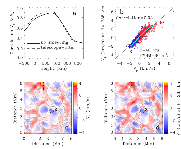
Figure 6: Comparison of the snapshot vertical velocities $V_{z}$ with the Dopplergram velocities $V_{P}$ inferred from the DOT-like data. (a): Correlation coefficients between $V_{P}$ and $V_{z}$ as a function of height for the case of no smearing (solid line) and telescope+filter smearing (dashed line). (b): Dopplergram velocities $V_{P}$ vs. snapshot velocities $V_{z}$. The latter were taken at heights where the correlation between $V_{P}$ and $V_{z}$ reaches maximum. Blue crosses are granular points and red circles are intergranular points. The light blue curve is the average over bins with 100 surface points. (c): Map of the Dopplergram velocities $V_{P}$. Circles with numbers (1), (2) correspond to the spatial points where the emergent profiles have high red and blue shifts, respectively. Those profiles are shown in Figure 8. Red denotes downflows and blue, upflows. (d): Map of the snapshot velocities $V_{z}$.

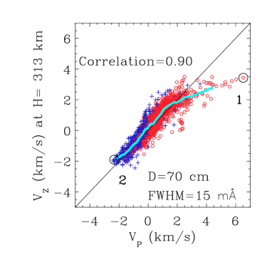
Figure 7: Comparison of the snapshot vertical velocities $V_{z}$ with the Dopplergram velocities $V_{P}$ inferred from the “speckle-reconstructed” VTT-like data.

Interestingly, with the narrower bandwidth and larger diameter of the telescope than in the case of the DOT observations the overestimation of the Doppler velocities $V_{P}$ in intergranular areas with strong downflows found from the “speckle-reconstructed observations” turns out to be appreciably larger. We display such a case for VTT-like data in Figure 7. As follows from the Figure, the deviation reaches approximately 3 km/s.

Figure 8: Ba ii 4554 Å line profiles at two selected locations corresponding to a high downflow (left) and a high upflow (right), marked by (1) and (2) in Figure6. (a, c): profiles without smearing. Thin lines with dots: parabolic fit to the five wavelength positions $\Delta\lambda=-70$, $-35$, 0, 35 and 70 mÅ indicated by black circles. Open circles: bisector of the Ba ii  profile; thin vertical line: bisector of the parabolic fit. The horizontal lines are full spectral line widths $\Delta{\lambda}_{W}=\Delta{\lambda}_{r}-\Delta{\lambda}_{b}$ specifying the wavelength distances between equal intensity points in the red and blue line wings. (b, d): same but for the DOT-like smeared profiles. $x_{i}$ and $y_{i}$ are the locations of the selected grid-points in the 3D-snapshot.

Figure 8 explains why such bright patches can arise in speckle-reconstructed observations and why it happens specifically in intergranular areas. It displays examples of the parabolic fit to the five fixed wavelength points of the original profiles (top) and DOT-like smeared profiles (bottom). The profiles are taken at the spatial locations marked (1) and (2) in Figure 6b, c, d. The profile marked (1) originates from the area with a high intergranular downflow (left) and the profile marked (2) originates from the area with a high granular upflow (right). According to Fig. 8a, it seems impossible to measure correctly the velocity from the weak twisted intergranular profile provided that the strong redshift forces four of the five wavelength points used for fitting to be situated in the blue wing. As a consequence, the parabola turns out to be much more redshifted than the original profile. So the Dopplergram velocity derived from the wavelength position of the parabola bisector (thin vertical line) will be considerably greater compared to the velocity inferred from the bisector of the original profile (small open circles). Smearing caused by the telescope and filter to some degree smoothes the irregular shape of the intergranular profile and decreases the redshift of the parabola (Fig. 8b). Nevertheless, the velocity remains overestimated. Thus, we conclude that the Dopplergram velocities calculated from the speckle-reconstructed DOT-like data in intergranular lanes can be appreciably greater than the real ones.

Contrary to the intergranular profile the deep and more symmetric granular profile allows us to estimate the velocity from the parabolic fit rather well (Fig. 8c). The effects of smearing are less pronounced in this case (Fig. 8d). So in granular areas with strong upflows one can expect a reasonable agreement between the “true” velocities $V_{z}$ and velocities $V_{P}$ recovered from the DOT-like data.

Summarizing the conclusion of this Section, the five-point Dopplergram technique applied to the Ba ii 4554 Å line profiles in speckle-reconstructed DOT-like data is a valuable tool for the diagnostic of the solar velocity field at heights around 300 km. Only in intergranular lanes with strong downflows can the velocity be overestimated producing artificially bright points at the Dopplergram velocity maps like those obtained by Sütterlin et al. (2001). These authors interpreted the bright points as locations of the magnetic flux tubes. However, our calculations show that at least part of such bright points may be simply an artefact caused by the parabolic fit.

5 $\lambda$-meter technique

The $\lambda$-meter method of Stebbins & Goode (1987) can be considered as a form of the “bisector shift” technique proposed earlier by Kulander & Jefferies (1966) to evaluate the atmospheric velocity field from the asymmetries in observed line profiles. The $\lambda$-meter method deals with two line profile parameters such as the line bisector and the full spectral line width $\Delta{\lambda}_{W}$.

The displacement of a midpoint of a section of the line profile of a certain width $\Delta{\lambda}_{W}$ is assumed to be a result of the Doppler shift of the line opacity coefficient caused by the non-thermal velocities in the layer where this section is formed. According to Stebbins & Goode (1987) the velocities and intensities from progressively deeper sections of the line profile correspond to progressively higher layers in the atmosphere. Following the $\lambda$-meter procedure we introduced a set of line profile widths $\Delta{\lambda}_{W}$ ranging from 306 to 78 mÅ (see Fig. 8). Due to the irregular shape of the Ba ii 4554 Å line core, a significant number of synthetic profiles never have a spectral line width lower than 78 mÅ. At the same time shallow far wings of many profiles do not allow us to detect and analyse velocities at widths above $\Delta{\lambda}_{W}=306$ mÅ. The selected $\Delta{\lambda}_{W}$ range corresponds to the intensities of spatially averaged profile varying between 0.86 and 0.16. The corresponding range of the mean formation heights lies between $\sim-50$ and $\sim 500$ km.

Figure 9: Correlation coefficients between $\lambda$-meter velocities $V_{\lambda M}$ and snapshot velocities $V_{z}$ as a function of the line profile width $\Delta{\lambda}_{W}$. The snapshot velocities are taken at heights $H$ where optical depth at the corresponding wavelength $\tau(\Delta{\lambda}_{b(r)})$ equals unity (see Sect. 2.2). Each line corresponds to a different value of $R_{0}$. The uppermost solid line refers to the case of no smearing. Left panel: blue wing velocities; right panel: red wing velocities. The VTT-like data are used.

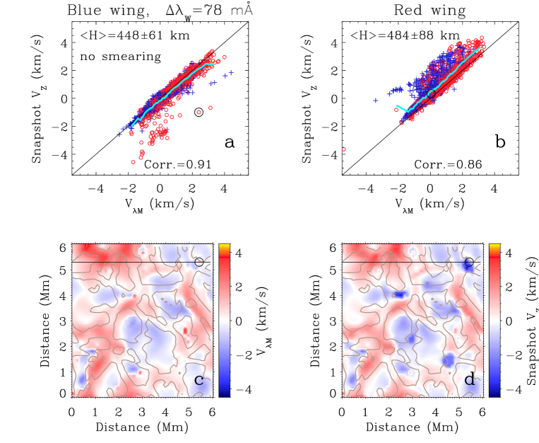
Figure 10: Comparison between the $\lambda$-meter velocities $V_{\lambda M}$ at $\Delta\lambda_{W}=$ 78 mÅ and snapshot velocities $V_{z}$, measured at corresponding heights $H$ for the case of no smearing. (a): Scatter plot of $V_{\lambda M}$ and $V_{z}$ in the blue wing. Black open circle marks the location $x_{i}=5.5$ Mm, $y_{i}=5.4$ Mm. (b): Same for the red wing velocities. (c): Map of the blue wing $V_{\lambda M}$. (d): Map of the snapshot velocities $V_{z}$ corresponding to the blue wing. The colour coding is the same as in Figure 6.

We slightly modified the standard $\lambda$-meter procedure keeping in mind that velocity field shifts the line opacity coefficients of various atmospheric layers towards one wing of the static line and away from the other. Such a shift expands the optical line depth $\tau(\Delta{\lambda})$ on one side of the line and compresses on the other side. As a consequence, the height of formation of the equal intensity points in the blue $\Delta{\lambda}_{b}$ and red $\Delta{\lambda}_{r}$ wings belonging the same spectral width $\Delta{\lambda}_{W}$ tends to be different. Our modified $\lambda$-meter procedure is the following. We applied the above set of spectral widths both to the spatially averaged profile and to the individual profiles over the snapshot. The spatially averaged profile corrected for asymmetry due to granulation velocity field (see Fig. 2, bottom) was considered as a reference profile representing a stationary case. Since our study deals only with the relative changes of the Ba ii 4554 Å line parameters no correction for the asymmetry caused by the hyperfine structure and isotopic shift was made. We derived the $\lambda$-meter velocities $V_{\lambda M}$ in the blue wings by measuring the Doppler shift of the blue intensity point belonging a certain spectral width relatively the corresponding blue point of the spatially averaged profile (same applies to the red wings).

The velocities $V_{\lambda M}$ obtained by this method were compared to the corresponding snapshot velocities $V_{z}$. The $V_{z}$ values were specified separately for the blue $\Delta{\lambda}_{b}$ and red $\Delta{\lambda}_{r}$ wavelengths belonging the same line width. These velocities were taken at heights where the optical depth at the corresponding wavelength points was equal to unity (see Sect. 2.2). The results of these calculation are displayed in Figs 9 to 14.

5.1 $\lambda$-meter: original resolution

Figure 9 shows the correlation coefficients between the maps of $\lambda$-meter velocities $V_{\lambda M}$ and the snapshot velocities $V_{z}$ taken at corresponding heights. It gives several cases for different seeing conditions (value of the parameter $R_{0}$) for the VTT-like data and also the case of no smearing. When the smearing is absent, the correlation coefficient for both blue and red wing velocities is rather high. It reaches a maximum value of $\sim 0.97$ around $\Delta{\lambda}_{W}=200$ mÅ, being slightly smaller in the inner wing of the line.

The scatter plots and maps of the $V_{\lambda M}$ and $V_{z}$ velocities in the inner wing of the line at $\Delta{\lambda}_{W}=78$ mÅ are presented in Fig. 10 for the case of no smearing. As follows from panel (a) of this figure, in the inner blue wing $\lambda$-meter velocities agree essentially with the true snapshot velocities at that height in most of the grid points. The correlation coefficient between them is very high and is close to 0.9. The comparison of the velocity maps in panels (c) and (d) supports this conclusion. Nevertheless, there is a set of grid points belonging mainly to intergranular lanes where the fit is fairly bad. The map of the true velocities $V_{z}$ in Fig. 10d reveals the presence of a number of intergranular lanes (as defined by the continuum intensity) where the upflowing velocities are observed at heights of formation of the blue wing intensity at $\Delta{\lambda}_{W}=78$ mÅ. The $\lambda$-meter velocities do not recover such upflowing points well, suggesting significantly smaller absolute value of the velocities or even their sign reversal. An example of such a location is marked by an open circle in Figure 10.

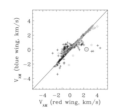
Figure 11: Scatter plot of the red and blue wing $\lambda$-meter velocities at $\Delta\lambda_{W}=$ 78 mÅ in the case of no smearing. Black crosses are granular points and light circles are intergranular points. the black open circle marks the point corresponding the location $x_{i}=5.5$ Mm, $y_{i}=5.4$ Mm shown in Fig. 10.

Figure 10b demonstrates that in the red inner wing the match between $V_{z}$ and $V_{\lambda M}$ is appreciably worse. The $\lambda$-meter velocities tend to be more redshifted. According to Fig. 11, the blue and the red wing $V_{\lambda M}$ are essentially the same (except for a few grid points), whereas the corresponding $V_{z}$ are not. The reason for that lies in the different formation heights of the blue and red wing intensities at the same $\Delta{\lambda}_{W}$ (we discuss this point in more details in Sect. 5.3). The velocities measured by the $\lambda$-meter technique correspond better to the heights where the blue-wing intensities are formed.

Figure 12a, b gives two more examples of the correlation between the $\lambda$-meter velocities and the snapshot velocities in the outer wings of the line. The match is typically rather good and the correlation is high, except that the amplitudes of the $\lambda$-meter velocities are systematically lower. The latter is easy to understand bearing in mind that the method gives the average information over a certain height range, thus leading to a decrease in the amplitude.

In summary, under perfect conditions, the $\lambda$-meter technique allows us to obtain information about the LOS velocities with a rather good precision over the whole photosphere, the agreement being a little worse for the inner wings of the line. The blue and the red wing $V_{\lambda M}$ velocities are very close to each other.

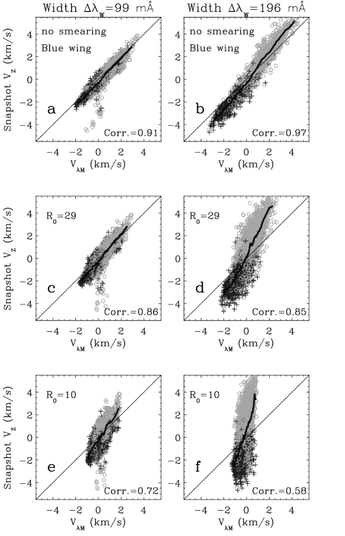
Figure 12: Scatter plot of the $\lambda$-meter velocities $V_{\lambda M}$ and the snapshot velocities $V_{z}$ in the wings of the line at $\Delta{\lambda}_{W}=99$ mÅ (left panels) and $\Delta{\lambda}_{W}=196$ mÅ (right panels) for the VTT-like data. (a and b): no smearing; (c and d): Fried’s parameter $R_{0}=29$; (e and f): $R_{0}=10$. The gray scale coding is the same as in Fig. 11.

5.2 $\lambda$-meter: reduced resolution

Apart from the case of the original resolution discussed above, Fig. 9 contains the calculation of the correlation coefficients between $V_{z}$ and $V_{\lambda M}$ for the VTT-like data smeared to have a different spatial resolution by varying the Fried parameter from 38 to 10 cm. As expected, the correlation coefficient gets lower compared to the case of perfect seeing conditions. Nevertheless, even for the medium spatial resolution ($R_{0}=10$ cm) the correlation for the inner wings ($\Delta{\lambda}_{W}=100$ mÅ) is rather high ($\sim 0.7$). For the higher values of $R_{0}$ the correlation coefficient increases up to 0.8–0.9. Opposite the case for no smearing, the correlation coefficient decreases from the inner to the outer wings. The velocity measured in the outer wings ($\Delta{\lambda}_{W}>120$ mÅ) is less precise.

The effects produced by the spatial smearing on the amplitudes of the measured velocities $\Delta{\lambda}_{W}$ are shown in Figure 12. The following points can be underlined from this Figure:

• In the original data the maximum absolute values of the velocities are higher above intergranular lanes than above granules. Spatial smearing reduces both the absolute values of the velocities and the asymmetry in the scatter plots. Nevertheless, the velocity asymmetry is still present.

• Even under excellent seeing conditions ($R_{0}=29$ cm) the outer wing $\lambda$-meter velocities for $\Delta{\lambda}_{W}>120$ mÅ are less reliable that the inner wing velocities.

• The inner wing velocities ($\Delta{\lambda}_{W}<120$ mÅ) still give a fairy good measure of the true velocities for the Fried parameter ($R_{0}=10$ cm).

• As the inner wings of the line are less sensitive to spatial smearing, the Ba ii 4554 Å line can be useful to measure velocities mainly in the upper photosphere.

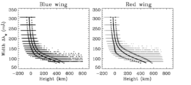
Figure 13: Formation heights of the intensity along the line profiles calculated for a set of spectral widths in the blue (left) and red (right) wings for all grid points from the 3D snapshot. Thick solid lines and open circles: mean formation heights and their standard deviation, respectively.

5.3 Intensity formation heights along the line profile

The $\lambda$-meter technique only yields qualitative results as long as it is not accompanied by the knowledge of heights where the information on the velocity and intensity variations comes from. In this section we give the results of the calculation of such heights. We calculated the Eddington–Barbier formation heights (see Sect. 2.2) for the intensity at each section of the Ba ii 4554 Å line profile having a certain spectral width $\Delta{\lambda}_{W}$. Below we use the notation $H_{b}$ for the blue wing intensity formation heights calculated at $\Delta{\lambda}_{b}$ positions in the blue wing, and similarly for the red wing intensity formation heights $H_{r}$, calculated at $\Delta{\lambda}_{r}$ positions in the red wing. Both $H_{b}$ and $H_{r}$ correspond to the same $\Delta{\lambda}_{W}$. We repeated the calculation for the all grid points of the 3D snapshot. The results of such calculations are presented in Figures 13 and 14. These figures give an answer to several important questions.

Firstly, how realistic is to assume that $H_{b}$ and $H_{r}$ belonging to the same $\Delta{\lambda}_{W}$ are constant over the 3D snapshot? The results shown in Fig. 13 suggest that this assumption is far from reality. At each fixed $\Delta{\lambda}_{W}$, both $H_{b}$ and $H_{r}$ vary in a rather wide range. In outermost sections of the profile ($\Delta{\lambda}_{W}=306$ mÅ) the heights vary between about $-175$ km and $+75$ km, while in the inner section ($\Delta{\lambda}_{W}=78$ mÅ) the range of the variations is larger and lies between $+300$ km and $+800$ km. Despite the large scatter, the mean formation heights of the each section of the profile $\left<H\right>$ have a well pronounced dependence on $\Delta{\lambda}_{W}$ (thick solid curves in Fig. 13). This makes it possible to assign in, a certain way, a height dependence to the velocity measurements by $\lambda$-meter technique. This can be done by ascribing the response of each $\Delta{\lambda}_{W}$ section of the spectral line to the mean height $\left<H\right>$.

Secondly, is it correct to assume that the $H_{b}$ and $H_{r}$ formation heights belonging to the same $\Delta{\lambda}_{W}$ are equal? In order to answer this question, we show in Fig. 14 two representative cases for $H_{b}$ and $H_{r}$ calculated at two positions in the inner ($\Delta{\lambda}_{W}=99$ mÅ) and the outer ($\Delta{\lambda}_{W}=196$ mÅ) wings of the line. The $\Delta{\lambda}_{W}=196$ mÅ corresponds to the section of the Ba ii 4554 Å where the line opacity profile is shallow. So one can expect the difference in heights of formation $H_{b}$ and $H_{r}$ caused by the Doppler shift of the opacity profile to be small. The width $\Delta{\lambda}_{W}=99$ mÅ belongs to the inner section of the Ba ii 4554 Å characterized by a steeper part of the line opacity profile. It is expected that the same Doppler shifts produce a more important difference in the optical depths on opposite sides of the Ba ii 4554 Å line and, hence, a somewhat greater difference between the $H_{b}$ and $H_{r}$ heights. What is the magnitude of this difference?

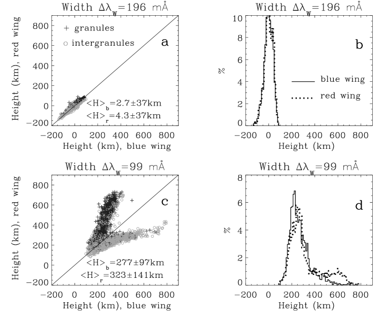
Figure 14: (a, c): Formation heights of the blue wing intensities vs. formation heights of the red wing intensities at two spectral widths: $\Delta{\lambda}_{W}=196$ mÅ and $\Delta{\lambda}_{W}=99$ mÅ. Dark crosses - granular points; light circles - intergranular points. (b, d): Histograms of the formation heights of the blue wing intensities (solid line) and red wing intensities (dotted line) for the same $\Delta{\lambda}_{W}$.

As follows from Fig. 14a, in the outer wings of the Ba ii 4554 Å line the blue $H_{b}$ and red $H_{r}$ heights are indeed very close to each other, both varying over the 3D snapshot. The histograms displayed in Fig. 14b demonstrate that the distributions of $H_{b}$ and $H_{r}$ are similar and have a sharp cut off. It means that outer wings are formed in a narrow atmospheric layer with mean heights $\left<H_{b}\right>$ and $\left<H_{r}\right>$ of the blue and red wings being very close to each other.

Figure 14c shows a similar calculation for the inner sections of the Ba ii 4554 Å line. The Doppler shift of the line opacity profile leads to a complex behaviour of the $H_{b}$ and $H_{b}$ heights. Two groups of points can be distinguished in the scatter plot of $H_{r}$ vs. $H_{b}$ calculated over the snapshot. For the first group (symbols above diagonal), the $H_{b}$ heights are concentrated in a rather narrow band around $+200$ km while the $H_{r}$ heights extend for several hundreds of kilometres from nearly $+100$ km to $+800$ km. This group of points belong largely to the profiles coming from granular regions. For the second group of points (symbols below the diagonal) the behaviour is the opposite. This group originates mostly in intergranular lanes. Only a relatively small number of the profiles have approximately the same $H_{b}$ and $H_{r}$ heights (symbols along the diagonal).

The histograms of the $H_{b}$ and $H_{r}$ heights for the inner sections of the Ba ii 4554 Å line (Fig. 14d) are not symmetric. The histograms have a maximum at heights around $+200$ km and a sharp cut-off below this height. There is a long tail toward 600–800 km. This tail is more pronounced for the red wing heights $H_{r}$. Such an asymmetry suggests that the information in the inner wing comes from two distinct layers. In most of the grid points the intensity at $\Delta{\lambda}_{W}=99$ mÅ is formed around $+300$ km, whereas in a smaller but still appreciable number of points the intensity comes from higher layers between $+400$ and $+800$ km. On the whole, the mean formation height of the inner red wing is larger than that of the inner blue wing.

6 Conclusions

In this paper we have analysed the range of validity of the two Doppler diagnostic techniques using the Ba ii 4554 Å line, i.e. the 5-point Dopplergram technique (Sütterlin et al., 2001) and the $\lambda$-meter technique (Stebbins & Goode, 1987). We have performed NLTE radiative transfer calculations of the Ba ii 4554 Å intensity profiles in the 3D snapshot of hydrodynamical simulations of solar convection (Asplund et al., 2000a), neglecting the effects of horizontal radiative transfer, but considering a realistic barium atomic model and taking into account the hyperfine structure and isotopic shift. The original resolution profiles were smeared to reproduce the DOT-like and VTT-like data and study the effects of the limited resolution into the reliability of the results produced by the two Doppler diagnostic techniques.

Our results for the 5-point Dopplergram technique can be summarized as follows:

• The NLTE simulations using the 3D hydrodynamical model support the opinion that the speckle-reconstructed Dopplergram velocities obtained from the DOT-like data give appropriate representation of the solar photospheric velocity field.

• The information on the velocities obtained from such Dopplergrams comes from a thin atmospheric layer located at heights around 300 km. The speckle-reconstructed Dopplergram velocity maps reproduce in many details the “true” velocity structures existing in this layer.

• The Dopplergram technique can overestimate the velocities in intergranular areas with strong downflows. This excess appears in the speckle-reconstructed maps as localized points with enhanced brightness. The interpretation of such bright points in terms of magnetic fields has to be carried out with caution. At least some of them may be an artefact caused by the Dopplergram technique itself.

Our conclusions regarding the $\lambda$-meter technique are the following:

• Under perfect seeing conditions the $\lambda$-meter technique allows us to obtain information about the LOS velocities throughout the photosphere with rather good precision. Only in the upper photosphere is the particular velocity structure with upflowing points in intergranular lanes not always well reproduced.

• The velocities measured by the $\lambda$-meter technique correspond better to the “true” snapshot velocities taken at heights of formation of the blue line wing, rather that the red wing.

• Even for rather medium seeing conditions the inner wings of the Ba ii 4554 Å line give reliable information about the velocity field in the upper photosphere. The results from the outer wings are less reliable.

• The mean formation heights of each section of the Ba ii 4554 Å line profile have a well-pronounced dependence on the spectral width of the section. This gives the possibility to assign height dependence to the velocity measurements by the $\lambda$-meter technique. The non-thermal motions can be reliably measured with the $\lambda$-meter technique applied to the Ba ii 4554 Å line throughout the photosphere up to the temperature minimum.

Appendix A NLTE modeling

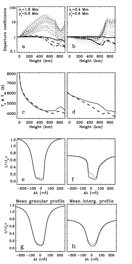
Figure 15: (a, b): Departure coefficients $\beta$ of the Ba ii atomic levels vs. height in a representative granular (left) and intergranular (right) models. Thick solid and thick dash lines: the $\beta$-coefficients for the ground $6s\,\rm{{{}^{2}}S}_{1/2}$ and upper $6p\,\rm{{{}^{2}}P}_{3/2}$ levels of the Ba ii 4554 Å line, respectively. Dash-dotted lines: the $\beta$-coefficients for the upper level of the Ba ii 4934 Å resonance line. Dotted lines: the $\beta$-coefficients for the Ba ii levels with excitation potentials above 5 eV. (c, d): The line source function $S_{L}$ of the Ba ii 4554 Å line (dash) and Planck function $B$ (solid) in units of the temperature vs. height for the same models. (e, f): The Ba ii 4554 Å line profiles for the representative granule and itergranule. Solid and dotted lines: NLTE and LTE, respectively. (g, h): Spatially averaged granular and intergranular profiles.

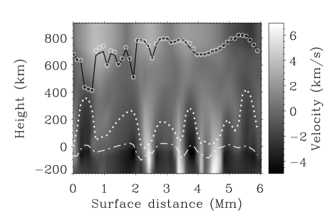
Figure 16: The NLTE (solid line) and LTE (open circles) heights of formation of the core of the Ba ii 4554 Å line along the slice of the snapshot $y_{i}=0.6$ Mm. Dash-dotted line: continuum height of formation at 4554 Å. Dotted line: height of formation of the line wing for the wavelength position $\Delta\lambda=-76.5$ mÅ. The background image is the snapshot vertical velocity $V_{z}$. Negative (upflow) velocities $V_{Z}$ correspond to granules (dark), while positive (downflow) velocities to intergranules (light).

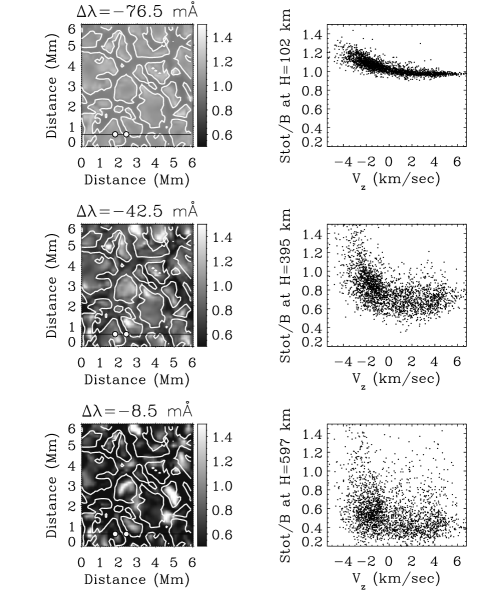
Figure 17: The total source function $S_{tot}(\Delta\lambda)/B$ measured in the Planck function units for three wavelength points $\Delta\lambda=-76.5;-42.5;-8.5$ mÅ situated in the blue wing of the Ba ii 4554 Å line profile. Left: Maps of the $S_{tot}(\Delta\lambda)/B$ at the mean intensity formation heights at these wavelengths. Horizontal line corresponds to the slice $y_{i}=0.6$ Mm and the filled circles to the surface positions $x_{i}=1.8$ Mm (granule), $x_{i}=2.4$ Mm (intergranule). Right: Scatter plots of $S_{tot}(\Delta\lambda)/B$ and velocities $V_{z}$ for the same wavelengths. The velocities are taken at heights of formation of continuum intensity.

Figure 15 (panels a to f) shows the population departure coefficients, the Ba ii $\lambda$4554 Å line source functions and line profiles for two spatial grid points of the 3D snapshot representing the typical granular and intergranular models. We use these models to illustrate the difference in the NLTE results for granules and intergranules. The population departure coefficients are defined as $\beta=n_{\rm NLTE}/n_{\rm LTE}$ where $n_{\rm NLTE}$ and $n_{\rm LTE}$ are the NLTE and LTE atomic level populations, respectively. The Complex behaviour of the $\beta$-coefficients shown in Fig. 15a, b is a result of the interaction of several NLTE mechanisms described in detail by Carlsson et al. (1992); Bruls et al. (1992); Shchukina & Trujillo Bueno (2001). Here we just point out that for the barium atom the most important of them are ultraviolet line pumping, ultraviolet overionization, resonance line scattering and photon losses. The resonance line scattering and photon losses manifest themselves as a divergence of the lower $6s\,\rm{{{}^{2}}S}_{1/2}$ and upper $6p\,\rm{{{}^{2}}P}_{1/2}$, $6p\,\rm{{{}^{2}}P}_{3/2}$ levels of the Ba ii resonance lines. This divergence results from the surface losses near the layer where the optical depth is equal to unity. The losses propagate by scattering to far below that layer. Interestingly, for the integranule the divergence of the $\beta$-coefficients arises in the innermost layers. This happens because the photon losses occur mainly through the line wings of the Ba ii 4554 Å line. As follows from Fig. 16 the line wings in integranules are formed considerably deeper than in granules. Such a difference in the formation heights is a result of the Doppler shift of the line opacity coefficient caused by the velocity field. As a consequence, in the intergranular model (see Fig. 15, a, b) the divergence starts already in the lower photosphere while in the granular model it happens only in upper photosphere at heights around 400 km.

Another important conclusion that follows from Fig. 16 concerns the height of formation of the Ba ii 4554 Å line. The lower departure coefficient $\beta_{l}$ is close to unity. So the scaling of the line opacity with this coefficient cannot lead to an appreciable difference between the NLTE and LTE heights of formation of this line.

The excess of Ba ii  ions at the levels with excitation potentials above 5 eV visible in the granule model is produced by the pumping via the ultraviolet Ba ii  lines starting at $6s\,\rm{{{}^{2}}S}$, $5d\,\rm{{{}^{2}}D}$, $6p\,\rm{{{}^{2}}P}^{o}$ levels. For the intergranule model the overpopulation arises only in the uppermost layers. Such behaviour of the $\beta$-coefficients corresponds to the temperature stratification of the models. The overpopulation of the high excitation levels of Ba ii in granules occurs because here the excitation temperature of the ultraviolet pumping radiation field appreciably exceeds the electron temperature. In integranules such superthermal radiation, and hence the level overpopulation, is present only above the temperature minimum region. In addition, in the intergranular photospheric layers the photon losses in the ultraviolet lines are more pronounced than in granules.

The ${\beta}_{u}/{\beta}_{l}$ ratio of the upper and lower level departure coefficients of the Ba ii 4554 Å line sets the departure of its line source function $S_{L}$ from the Planck function $B$. Figure 15 (c, d) shows that this departure (reflecting the corresponding departure coefficient divergence in the upper panels of this Figure) is larger in the intergranular than in the granular model.

Figure 17 demonstrates that such behaviour is typical also for the total source function $S_{\rm{tot}}$ at the wavelengths corresponding to the inner wings ($\Delta\lambda<76.5$ mÅ). On average, in intergranular regions it drops below the Planck function while in granules the effect is less pronounced. Moreover, in granular areas with strong upflows the total source function can exceed the Planck function. This excess can be understood if one takes into account that the resonance source line function is described by the two-level approximation, i.e. it approximately equals mean intensity $J$. In the regions with small photon losses (like granules) the $J>B$, hence, $S_{L}$ and $S_{\rm{tot}}$ have to be greater than $B$ as well.

Figure 15 (e, f) show the NLTE and LTE disc-centre line profiles for the individual granular and integranular models. The profiles displayed in Fig. 15 (g ) result from averaging of the emergent intensities corresponding only to the granular models. Averaged intergranular profiles are shown in Figure 15 (h). These two bottom panels quantify the statistical effect produced by the deviation from the LTE in two such types of the atmospheric models. The main conclusions that may be drawn from the results presented in Fig. 15, 16, 17 are the following:

• The source function deficit, as compared to the LTE assumption, is the main mechanism that controls the formation of the Ba ii $\lambda$4554 Å  line. The line opacity deficit is small and, hence, unimportant.

• The divergence between $S_{tot}$ and $B$ changes the shape of the individual profiles, particularly the intergranular ones.

• On average, the deviations from the LTE lead to deepening (i.e. strengthening) of the spatially averaged Ba ii $\lambda$4554 Å line profiles. The NLTE effects are most pronounced around the line core and are generally more important in the intergranular regions than in the granular ones. The mean difference between the NLTE and LTE line core residual intensities does not exceed 5% for granules and 10% for intergranules.

• Towards the wings, the LTE becomes a valid description for the Ba ii $\lambda$4554 Å  line profile.