Localization properties of one-dimensional Frenkel excitons:
Gaussian versus Lorentzian diagonal disorder

Abstract

We compare localization properties of one-dimensional Frenkel excitons with Gaussian and Lorentzian uncorrelated diagonal disorder. We focus on the states of the Lifshits tail, which dominate the optical response and low-temperature energy transport in molecular J-aggregates. The absence of exchange narrowing in chains with Lorentzian disorder is shown to manifest itself in the disorder scaling of the localization length distribution. Also, we show that the local exciton level structure of the Lifshits tail differs substantially for these two types of disorder: In addition to the singlets and doublets of localized states near the bare band edge, strongly resembling those found for Gaussian disorder, for Lorentzian disorder two other types of states are found in this energy region as well, namely multiplets of three or four states localized on the same chain segment and isolated states localized on short segments. Finally, below the Lifshits tail, Lorentzian disorder induces strongly localized exciton states, centered around low energy sites, with localization properties that strongly depend on energy. For Gaussian disorder with a magnitude that does not exceed the exciton bandwidth, the likelihood to find such very deep states is exponentially small.

I Introduction

The term ”exciton”, introduced seventy-five years ago in the pioneering works of Frenkel Frenkel32 and Wannier, Wannier37 has become widely used to explain optical and transport properties of a large variety of organic and semiconductor materials. Knox63 ; Davydov71 ; Agranovich82 Within this general context, low-dimensional (nanoscale) systems currently attract particular attention.Scholes06

In low-dimensional systems, an important factor influencing the exciton states is the presence of disorder, which results from static fluctuations in the host, different growth conditions, as well as imperfections of the systems themselves. Disorder induces localization of the exciton states Anderson58 ; Kramer93 on certain segments of the system; the linear extent of such segments is usually referred to as the localization length. These localized states consequently lead to the appearance of tails in the density of states (DOS) outside of the bare exciton band, which are commonly known as Lifshits tails. Halperin66 These states play a key role in the low-temperature energy transport as well as in the optical properties of a wide spectrum of materials, such as conjugated oligomer aggregates Spano06 and polymers, Hadzii99 molecular J-aggregates, Kobayashi96 semiconductor quantum wells and quantum dots, Takagahara03 semiconductor quantum wires, Akiyama98 as well as photosynthetic light harvesting complexes vanAmerongen00 and proteins. Berlin07

In discrete materials, characterized by interacting sites (molecular aggregates, conjugated polymers, photosynthetic complexes, spin systems), various types of disorder may be considered. Commonly used are uncorrelated diagonal (on-site) and off-diagonal disorder, where different choices still can be made for the types of disorder distributions; a Gaussian distribution and a box-like distribution are the most common choices. An interesting alternative is provided by a Lorentzian distribution, because the tight-binding model with diagonal uncorrelated Lorentzian disorder (known as the Lloyd model) is one of the few disorder models that allows for analytical calculation of several physical quantities, such as the averaged one-particle Green’s function Lloyd69 and the variance of the Lyapunov exponent, which is a measure of the localization length. Deych00 The details of the disorder model affect the optical response and transport properties of the above mentioned systems, sometimes substantially. While in comparison to Gaussian and box-like distributions the choice of Lorentzian disorder is not very common, it is worth noting that the latter naturally occurs in random systems dominated by dipolar interactions (see Appendix A).

In this paper, we perform a comparative study of uncorrelated Gaussian and Lorentzian diagonal disorder in one-dimensional excitonic systems, with particular interest in the localization properties, level structure, and statistics of the wave functions of the exciton states in the Lifshits tail. We will only consider moderate disorder magnitudes, where the exciton states still correspond to electronic excited states that are coherently shared by a number of molecules. There is an important difference between Gaussian and Lorentzian disorder: the former is characterized by a bounded second moment, while the second moment of the latter diverges. Distributions with a finite second moment give rise to exchange narrowing: Knapp84 because the exciton wave functions are coherently shared by a number ($N^{*}$) of monomers, they feel an effective disorder of magnitude $\sqrt{N^{*}}$ times smaller than the bare value. This effect explains the narrowness of the optical spectra of molecular J-aggregates as compared to their monomeric counterparts. Knapp84 Exchange narrowing does not occur for Lorentzian disorder. Eisfeld06 As we will show, this difference strongly affects the disorder scaling of the localization properties of the excitons, resulting in differences in the optical and transport properties. In addition, for Lorentzian disorder the relatively high density of sites with a very low energy (well outside of the exciton band), also plays an important role in the exciton optical dynamics.

The outline of this paper is as follows. In the next section, we present our model and analyze the exchange narrowing effect. Section III contains the results of numerical simulations and discusses the local level structure and the statistics of the wave functions in the Lifshits tail for Lorentzian disorder, which we compare to previously obtained results for Gaussian disorder. In Sec. IV, we discuss the scaling properties of the average as well as the standard deviation of the localization length in the Lifshits tail for both types of disorder. Section V summarizes the paper. In Appendix A we show that systems with random dipolar interactions provide physical realizations of the Lorentzian disorder model that is analyzed in this paper. Finally, in Appendix B, we present some mathematical details of derivations outlined in Sec. II.2.

II Theoretical background

II.1 Frenkel Hamiltonian

We consider a disordered Frenkel exciton chain of $N$ molecules, described by the Hamiltonian

$$\hat{H}=\sum_{n=1}^{N}E_{n}\left|n\rangle\langle n\right|-J\sum_{n=1}^{N-1}\left(\left|n\rangle\langle n+1\right|+\left|n+1\rangle\langle n\right|\right)\ .$$ (1)

Here $|n\rangle$ denotes the state in which molecule $n$ is excited, while all other molecules are in their ground state. $E_{n}$ denote the molecular excitation energies and $-J~{}(J>0)$ is the nearest-neighbor interaction. We neglect interactions beyond the nearest-neighbor, as this allows for an analytical discussion of several important quantities. In Sec. IV we will briefly comment on extension of the model to include long-range dipole-dipole interactions. We account for disorder by including a stochastic component in the site energies $E_{n}$. Two distributions of $E_{n}$ will be considered, a Gaussian and a Lorentzian, both with zero mean (the transition energy of an isolated molecule is set to zero)

$$G(E_{n})=\frac{1}{\sqrt{2\pi}\Delta_{G}}\ \exp\left(-\frac{E_{n}^{2}}{2\Delta_{G}^{2}}\right)\ ,$$ (2)

$$L(E_{n})=\frac{1}{\pi}\frac{\Delta_{L}}{E_{n}^{2}+\Delta_{L}^{2}},$$ (3a)

where $\Delta_{G}$ and $\Delta_{L}$ denote the standard deviation and half width at half maximum (HWHM), respectively, which are measures of the disorder strength.

For a given disorder realization, diagonalizing the Hamiltonian (1) yields the $N$ exciton wave functions $|\nu\rangle=\sum_{n=1}^{N}\varphi_{\nu n}|n\rangle$ and the corresponding energies $E_{\nu}$. For nonzero disorder strength, these exciton states will be localized on a length scale that depends on the energy. The linear optical response is dominated by the states with a large transition dipole to the ground state, i.e. with a large oscillator strength $O_{\nu}=\left(\sum_{n=1}^{N}\varphi_{\nu n}\right)^{2}$, where we have assumed that all molecular transition dipoles are equal, and the oscillator strength of a monomer is set to unity. These states occur in the neighborhood of the lower exciton band edge for the disorder-free system, $E_{b}=-2J$, mostly in the Lifshits tail, i.e., just below $E_{b}$. Their typical extension (localization length) is indicated by $N^{*}$. This quantity can also be interpreted as the typical number of coherently bound molecules participating in a particular exciton state.

There are various measures for the localization length of a particular exciton state. We will consider the one based on the inverse participation ratio Thouless74 ; Schreiber82 ; Fidder91 or participation number. The latter is defined as

$$N_{\nu}=\left(\sum_{n=1}^{N}\varphi_{\nu n}^{4}\right)^{-1}\ ,$$ (4)

which reflects the number of molecules that contribute to the exciton state $\left|\nu\right>$.

II.2 Exchange narrowing

A common property of systems of interacting molecules is that their delocalized excited states give rise to much narrower spectral peaks than an ensemble of noninteracting molecules. This phenomenon is referred to as exchange narrowing. Knapp84 Its origin lies in the fact that the delocalized excited states do not feel the local disorder magnitude, but rather an average over its variations, which leads to a reduced effective disorder. More specifically, for an exciton state spread over a localization segment of length $N^{*}$, the residual disorder strength is $\sigma=\Delta/\sqrt{N^{*}}$, where $\Delta$ is the standard deviation ($\Delta^{2}$ is the second moment of the disorder distribution).

For Lorentzian disorder, exchange narrowing does not occur because the second moment diverges, which results in the absence of the exchange narrowing effect. Eisfeld06 Below, we briefly sketch these arguments. For this purpose, we will use the Hamiltonian (1) on the basis of the exciton wave functions of a disorder-free linear chain,

$$|\nu\rangle=\left(\frac{2}{N+1}\right)^{1/2}\sum_{n=1}^{N}\sin\left(\frac{\pi\nu n}{N+1}\right)|n\rangle\ ,$$ (5)

with $\nu=1,2,...,N$. This yields

$$\hat{H}=\sum_{\nu=1}^{N}E_{\nu}|\nu\rangle\langle\nu|+\sum_{\nu\nu^{\prime}=1}^{N}H_{\nu\nu^{\prime}}|\nu\rangle\langle\nu^{\prime}|\ ,$$ (6a)

with

$$E_{\nu}=-2J\cos\left(\frac{\pi\nu}{N+1}\right)\ ,$$ (6b)

and

$$H_{\nu\nu^{\prime}}=\frac{2}{N+1}\sum_{n=1}^{N}E_{n}\sin\left(\frac{\pi\nu n}{N+1}\right)\sin\left(\frac{\pi\nu^{\prime}n}{N+1}\right)\ .$$ (6c)

$H_{\nu\nu^{\prime}}$ is a stochastic matrix fluctuating from one realization of the disorder to another. Its diagonal elements $H_{\nu\nu}$ describe fluctuations of the exciton energies due to disorder, while the off-diagonal part describes the scattering of excitons between different states, which eventually results in their localization. We are interested in the distribution functions $P(H)$ of these fluctuation matrix elements.

For Gaussian diagonal disorder, it is given by (see Appendix B)

$$P_{\nu\nu^{\prime}}(H)=\frac{1}{\sqrt{2\pi}k_{\nu\nu^{\prime}}\Delta_{G}}\exp\left(-\frac{H^{2}}{2k_{\nu\nu^{\prime}}^{2}\Delta_{G}^{2}}\right)\ ,$$ (7)

where $k_{\nu\nu}=1/\sqrt{(3/2)(N+1)}$ and $k_{\nu\nu^{\prime}}=1/\sqrt{N+1}~{}~{}(\nu\neq\nu^{\prime})$. Thus, the distribution function $P_{\nu\nu^{\prime}}$ is also a Gaussian with standard deviation $k_{\nu\nu}\Delta_{G}=\Delta_{G}/\sqrt{(3/2)(N+1)}$ and $k_{\nu\nu^{\prime}}\Delta_{G}=\Delta_{G}/\sqrt{N+1}$ for the diagonal and off-diagonal elements, respectively. The observed suppression of the bare disorder magnitude $\Delta_{G}$ by a factor of $\sqrt{N+1}$ reflects the exchange narrowing effect. Knapp84

By contrast, for Lorentzian diagonal disorder $P(H)$ reads (see, again, Appendix B)

$$P_{\nu\nu^{\prime}}(H)=\frac{1}{\pi}\>\frac{k_{\nu\nu^{\prime}}\Delta_{L}}{H^{2}+k_{\nu\nu^{\prime}}^{2}\Delta_{L}^{2}}\ ,$$ (8a)

where

$$k_{\nu\nu^{\prime}}=\frac{2}{N+1}\sum_{n=1}^{N}\left|\sin\left(\frac{\pi\nu n}{N+1}\right)\sin\left(\frac{\pi\nu^{\prime}n}{N+1}\right)\right|\ .$$ (8b)

As is seen, the distribution function of $H_{\nu\nu^{\prime}}$ is also a Lorentzian. For the diagonal elements, $k_{\nu\nu}=1$, independently of $\nu$, i.e., $P_{\nu\nu}(H)$ has the same width as the bare distribution (3a), which implies that there is no exchange narrowing in this case. The off-diagonal elements are distributed differently, depending on $\nu$ and $\nu^{\prime}$. For our purpose, namely theoretically estimating the localization length in the neighborhood of the lower band edge, only $k_{12}$ is relevant (see below). The analytical result reads $k_{12}=8/(3\pi)$, which does not show an exchange narrowing effect either. For arbitrary $\nu$ and $\nu^{\prime}$ the sum in Eq. (8b) can not be evaluated analytically. However, it can be seen that for large $N$ it scales linearly with $N$. Thus, in the limit of large $N$ the exchange narrowing effect is absent for all $H_{\nu\nu^{\prime}}$.

II.3 Estimates of the localization length

The expressions in the preceding section are valid generally. However, only in the perturbative limit, when $H_{\nu\nu^{\prime}}<|E_{\nu}-E_{\nu^{\prime}}|$, does it make sense to consider $|\nu\rangle$ as the (approximate) eigenstates and to interpret the widths of the distributions $P_{\nu\nu}(H)$ as linewidths for the absorption peak of that state. If this inequality does not hold, the off-diagonal matrix elements $H_{\nu\nu^{\prime}}$ mix the exciton states, resulting in their localization on segments of the chain. Obviously, the perturbative limit is never reached for infinite chains, as then the energy separations of states adjacent in energy get infinitesimally small. It has been shown, however, that the above mixing arguments lead to an excellent estimate of the typical exciton localization length near the bare band bottom if applied self-consistently to states within finite localization segments.Malyshev91 ; Malyshev95

The self-consistent argumentation is valid for states localized on chain segments much smaller than the chain length and much bigger than a single molecule ($1\ll N^{*}\ll N$). Two notions underly the reasoning: (i) States localized on the same chain segment undergo level repulsion, i.e., they have a finite energy difference. In particular, the energy separation between the two bottom states in a localization segment of length $N^{*}$ is approximately given by the energy difference $E_{2}^{*}-E_{1}^{*}$, where $E_{\nu}^{*}$ is given by Eq. (6b) for $N=N^{*}$. Here we used the fact that the states resemble those of a finite homogeneous chain with length $N^{*}$, in particular in the sense that the lowest exciton state on the segment has a wave function without nodes, while the next higher state has one node.Malyshev95 (ii) Two homogeneous basis states $\nu$ and $\nu^{\prime}$ localized on a chain segment of length $N^{*}$ are mixed by $H_{\nu,\nu^{\prime}}^{*}$ given by Eq. (6c) with $N$ replaced by $N^{*}$. The central argument in estimating the localization size near the band bottom is now that this size adjusts itself such that $H^{*}_{21}=E_{2}^{*}-E_{1}^{*}$. Namely, if $H^{*}_{21}<E_{2}^{*}-E_{1}^{*}$, the disorder would only be perturbative and the states would increase their spread. On the other hand, if $H^{*}_{21}>E_{2}^{*}-E_{1}^{*}$, the disorder would strongly mix the two states and would localize the exciton wave functions further.

As we have seen above, for Gaussian disorder, or any other disorder distribution with a bounded second moment, exchange narrowing of $H_{21}$ takes place, such that its typical value is $H^{*}_{21}=\Delta_{G}/\sqrt{N^{*}}$. Furthermore, assuming that $N^{*}\gg 1$ we have $E_{2}^{*}-E_{1}^{*}=3\pi^{2}J/N^{*2}$. Thus, the requirement $H^{*}_{21}=E_{2}^{*}-E_{1}^{*}$ leads to the estimate Malyshev91 ; Malyshev95

$$N^{*}=\left(3\pi^{2}\frac{J}{\Delta_{G}}\right)^{2/3}\ .$$ (9)

for the typical localization size. This power-law behavior is in excellent agreement with previous numerical calculations, Schreiber82 ; Fidder91 as well as with the analytical scaling relation obtained within the Coherent Potential Approximation (CPA). Boukahil90

For systems with Lorentzian disorder, no exchange narrowing occurs, i.e., $H^{*}_{21}=8\Delta_{L}/(3\pi)$. Now the requirement $H^{*}_{21}=E_{2}^{*}-E_{1}^{*}$ yields

$$N^{*}=\left(\frac{9\pi^{3}}{8}\frac{J}{\Delta_{L}}\right)^{1/2},$$ (10)

which reveals a different power-law scaling than for Gaussian disorder. In Sec. IV we will find that the $\Delta_{L}^{-1/2}$ scaling indeed agrees with numerical results.

While our main interest is in the optically dominant band-edge states, it is interesting to apply the above arguments also to the band center, and compare to previous results. Kramer93 ; Fyodorov92 Near the band center, $E_{\nu}^{*}-E_{\nu^{\prime}}^{*}\propto 2\pi J/N^{*}$, with $N^{*}$ now indicating the typical localization size at the band center. Equating this quantity to the exchange narrowed disorder strength, $\Delta_{G}/\sqrt{N^{*}}$, we find $N^{*}\propto(J/\Delta_{G})^{2}$. This indeed is the well known disorder scaling of the localization length in one-dimensional systems with Gaussian site disorder, Kramer93 which in Ref. Fyodorov92, has also been obtained by an analytical calculation of the inverse participation ratio, performed within the framework of a one-dimensional nonlinear supermatrix $\sigma$ model.

III Hidden spectral structure for Lorentzian disorder

As we mentioned above, the optically dominant states in a disordered exciton chain with negative transfer interactions occur in the neighborhood of the band bottom, predominantly in the Lifshits tail. The exciton states in this tail exhibit a hidden structure, Malyshev95 where doublets of $s$- and $p$-like states often occur on the same localization segments (and more rarely, triplets). As a result the low-temperature optical response of the chain behaves approximately as that of a collection of segments with typical size $N^{*}$ equal to the typical localization length of the optically dominant states. More detailed statistics were obtained in Ref. Malyshev01, , where the disorder scaling of the localization length, the oscillator strength, and the energy spacings $E_{2}^{*}-E_{1}^{*}$ were scrutinized numerically for Gaussian diagonal disorder. In this section, we report the results of similar numerical calculations with Lorentzian diagonal disorder and show that this both alters the hidden structure near the bare band bottom and induces a relatively high density of strongly localized low energy wave functions.

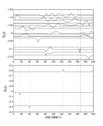
Figure 1: A realization of the low energy wave functions near the band bottom (upper panel) and well below it (lower panel) for a chain of $N=200$ sites and a Lorentzian distribution of site energies (HWHM $\Delta_{L}=0.05J$). In the upper panel three types of states are observed: (i) Multiplets of states (upper panel), (ii) states strongly localized on short segments, and (iii) states that form a conventional hidden level structure (see text for details). The solid vertical lines indicate the sites with large negative energy fluctuations, around which states deep in the tail are localized (lower panel): $n=5$, $n=16$, $n=40$, $n=125$, and $n=162$, while the dashed vertical line corresponds to the high energy site $n=168$. Two low energy exciton states (at $n=5$ and $n=162$) are not shown.

The exciton wave functions for a given realization of the disorder are straightforwardly obtained by diagonalizing the Hamiltonian Eq. (1), where we pick the site energies $E_{n}$ from a Lorentzian distribution Eq. (3a). In Fig. 1, we show a typical realization of the wave functions in the neighborhood of the bare exciton band edge $E_{b}=-2J$ (upper panel) and well below it (lower panel), calculated for $\Delta_{L}=0.05J$. It is clearly seen that the localization properties of these two subsets of wave functions differ substantially. The states near the band edge are much more extended than those deep in the tail and exhibit a hidden multiplet structure, similar to the case of Gaussian disorder. Malyshev95 ; Malyshev01 The important difference is that for Gaussian disorder, one usually finds only singlets and doublets of states localized on a particular chain segment. In the case of a Lorentzian distribution, on the other hand, we see the occurrence of multiplets of three and even four states, often on segments with sharply defined boundaries. It should be stressed that this situation is typical; looking at various realizations, we always found higher order multiplets. Below, we provide an explanation for this special property of Lorentzian disorder.

As we mentioned above, the states deep in the tail of the DOS (lower panel in Fig. 1) look different from those in the neighborhood of the band edge. They are, first, localized much more strongly (in fact, on a few sites, as can be seen by the eye and is confirmed by the participation number) and they are always represented by $s$-like singlets. These states originate from a large negative fluctuation of one particular site energy. For moderate disorder magnitudes, such fluctuations occur frequently for Lorentzian disorder, in contrast to Gaussian disorder.

Such outliers in energy have another consequence: they act as natural barriers, providing a segmentation of the chain into smaller subchains. In the realization of Fig. 1, these outliers occur at the positions $n=5$, $n=16$, $n=40$, $n=125$, $n=162$ and $n=168$. Segments between such barriers that happen to have a length of around the typical localization length $N^{*}$ of the band-edge states (upper panel), can easily support the formation of multiplets. For instance, a triplet of localized states occurs between $n=125$ and $n=162$, and a quartet is observed between $n=168$ and $n=200$. On the other hand, more strongly localized states may occur near the band edge as well. This happens if two closely spaced sites acquire large energy fluctuations, creating a segment considerably smaller than $N^{*}$. The states localized between $n=5$ and $n=16$ and between $n=162$ and $n=168$ represent two examples of this second type of exciton state. Finally, the segments that are appreciably larger than $N^{*}$ show a hidden level structure similar to that for Gaussian disorder, that is, where the localization segments have poorly defined boundaries and can be seen to overlap each other. This third type of exciton state can be seen in the segment between $n=40$ and $n=125$ in Fig. 1.

We proceed with a brief analysis of the wave functions of the exciton states deep in the tail of the DOS, which coincide with (some of) the aforementioned segment boundaries. These strongly localized states are centered around very low energy sites, and typically have localization lengths, as defined by the participation ratio in Eq. (4), of around a few sites. The wave functions decay approximately exponentially when one moves away from the central low energy site.

A simple model for these wave functions is given by a particle of mass $m$ moving in a $\delta$-function potential well. It is well known that such a well supports one bound state (with negative energy $E$), the wave function of which behaves proportionally to $\exp(-|x|/\xi)$ (see, e.g., Ref. Griffiths95, ). The relation between the penetration depth $\xi$ and the energy is given by Griffiths95

$$\xi=\sqrt{\frac{\hbar^{2}}{m}}\left(-E\right)^{-1/2}\ .$$ (11)

Clearly, the meaning of $\xi$ is similar to the localization length $N^{*}$; both are measures of the extent of the wave function. The localization length calculated through the participation number Eq. 4 is more suited for wave functions of unknown, arbitrary shapes. The known shape of the wave functions for the low-energy states, however, suggests to consider their exponential decay lengths and investigate whether their energy scaling resembles Eq. 11.

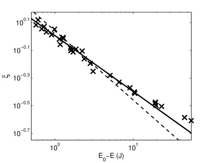
Figure 2: Double logarithmic plot of the numerically obtained penetration depth $\xi$ (in lattice units) as a function of energy $E_{0}-E$. The expected decay of the penetration depth with energy is clearly seen. The solid line shows a power law fit, while the dashed line represents the $\xi\propto\left(E_{0}-E\right)^{-1/2}$ behavior suggested by the $\delta$-function potential model.

As was shown in Refs. Klugkist08, and Klugkist07, , in the neighborhood of the bare exciton band edge, a universal energy variable $\tilde{\varepsilon}$ exists, which is given by

$$\tilde{\varepsilon}=\frac{\varepsilon-\varepsilon_{b}+a\sigma^{\alpha}}{b\sigma^{\alpha}}\ ,$$ (12)

where $\varepsilon=E/J$, $\varepsilon_{b}=E_{b}/J$ is the bare exciton band edge energy ($\varepsilon_{b}=-2$ for nearest-neighbor interactions), and the disorder strength $\sigma$ is either $\Delta_{G}/J$ or $\Delta_{L}/J$ for Gaussian and Lorentzian disorder, respectively. In terms of $\tilde{\varepsilon}$, functions of energy, like the DOS, become universal. The numerical coefficients $a$, $b$, and $\alpha$ depend on the type of disorder considered as well as on whether we include only nearest-neighbor or all dipole-dipole interactions. In particular, for nearest-neighbor interactions and Gaussian diagonal disorder, this set is given by $a=0$, $b=1$, and $\alpha=4/3$, Klugkist07 while in the case of nearest-neighbor interactions and Lorentzian diagonal disorder, we should use $a=1$, $b=4$ and $\alpha=1$. Klugkist07 We define a reference energy $E_{0}$ that is dependent on the disorder magnitude, which is the energy that corresponds to $\tilde{\varepsilon}=0$ on the universal energy scale.

An analysis of the numerically determined wave functions indeed confirms the expected general trend that the lower energy states are localized more strongly than the band edge states. For the deep tail energy states, the penetration depth $\xi$ was calculated by fitting an exponential to the numerically determined wave function. The result is plotted in Fig. 2 against the state’s energy measured from the reference energy $E_{0}$. We observe that these data approximately obey a power law, although not with quite the same exponent as suggested by Eq. (11). The best fit was obtained using the power law $\xi(E)=1.017\left[(E_{0}-E)/J\right]^{-0.405}$. The deviation of the numerically determined exponent from the estimated power law is most likely caused by the fact that the $\delta$-function model assumes a continuous position variable and an infinitely narrow and infinitely deep well, while our model Hamiltonian is discrete and can thus only approximately behave as in the $\delta$-function model. We also note that the very low energy states are very symmetric, while the exciton states that are closer to the band edge show more asymmetry; this makes sense, since for the more energetic states the surrounding sites become more important, at the expense of the central low-energy site. As the energies of the surrounding sites are random, this leads to the observed asymmetry.

Summarizing this section, we point out that the nature of the localization in the Lifshits tail of the DOS for Lorentzian disorder clearly differs from the usual Gaussian model in a number of aspects, in particular, it alters the hidden level structure and introduces strongly localized states deep in the tail which are far less likely to occur for Gaussian stochastic variables. Close to the bare exciton band edge, we observe three types of states: strongly localized $s$-like states on segments much smaller than the localization length $N^{*}$, multiplets on segments of lengths comparable to $N^{*}$, and finally, states that resemble the conventional hidden level structure that is also found for Gaussian disorder. In the next section we provide a more detailed analysis of the scaling of the localization length for both types of disorder in the neighborhood of the bare exciton band edge.

IV Localization length distributions and scaling

The localization length of a given exciton state $|\nu\rangle$ can be calculated numerically using the participation number $N_{\nu}$, Eq. (4). It is a fluctuating quantity and is thus more accurately described by analyzing its probability distribution. We focus on the energy range where the optically dominant states reside, i.e., in the neighborhood of the bare exciton band edge, $E_{b}=-2J$, and predominantly, just below it. To ensure a fair comparison, we fix the endpoints of the energy interval under consideration in terms of the universal energy variable mentioned in Section III. In the following simulations, it ranges from $\tilde{\varepsilon}_{i}=-0.1$ to $\tilde{\varepsilon}_{f}=0$.

The probability distribution of the localization length collected in this energy region, $P(N_{loc})=\sum_{\nu}^{\prime}\delta(N_{loc}-N_{\nu})$ (the prime restricting the summation to the selected energy interval), are plotted in the insets of Fig. 3 (Gaussian disorder with $\Delta_{G}=0.2J$) and Fig. 4 (Lorentzian disorder with $\Delta_{L}=0.05J$). They show an asymmetric shape, similar to the one presented in Ref. Malyshev01, . The asymmetry is caused by the fact that on average, the states with smaller localization lengths reside deeper in the DOS tail, where the DOS itself is small. If we instead go towards the exciton band edge, the situation is reversed.

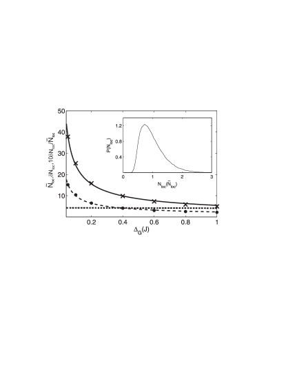
Figure 3: Disorder scaling of the average localization length (denoted by crosses) and its standard deviation of the distribution (denoted by the dots) for a chain of length $N=250$ sites with Gaussian disorder. Power law fits for both have been included: the solid line corresponds to $\bar{N}_{loc}=5.43\left(\Delta_{G}/J\right)^{-0.65}$, and the dashed line gives $\delta N_{loc}=2.33\left(\Delta_{G}/J\right)^{-0.63}$. Additionally, the quotient of the standard deviation and the average localization length is shown by the dotted line (multiplied by a factor of 10 for better visibility), which clearly shows this ratio to be constant to a good approximation. In the inset, we show the localization length distribution for $\Delta_{G}=0.2J$, plotted on a $N_{loc}$ scale which is normalized to $\bar{N}_{loc}$. The resulting function is universal, as it does not depend on $\Delta_{G}$ (see text).

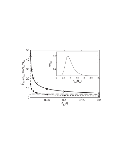
Figure 4: Same as in Fig. 3, but now for Lorentzian disorder with HWHM $\Delta_{L}$. The power law fits for the average localization length (solid line) and the standard deviation (dashed line) shown in the figure correspond to $\bar{N}_{loc}=2.19\left(\Delta_{L}/J\right)^{-0.48}$ and $\delta N_{loc}=0.80\left(\Delta_{L}/J\right)^{-0.46}$, respectively. The distribution in the inset was obtained for $\Delta_{L}=0.05J$.

Analyzing the moments of the various distributions indeed highlights the difference between the localization behavior for the two types of disorder, as predicted in Sec. II. In particular, for Gaussian disorder, we find $\bar{N}_{loc}=5.43\left(\Delta_{G}/J\right)^{-0.65}$, which has an exponent that is in good agreement with the theoretical power law Eq. (9). Lorentzian disorder, on the other hand, leads to the scaling with a different exponent, $\bar{N}_{loc}=2.19\left(\Delta_{L}/J\right)^{-0.48}$, again in good agreement with the theoretical estimate of Eq. (10), $N^{*}\approx 5.91\left(\Delta_{L}/J\right)^{-1/2}$. There is a deviation in the numerical prefactors, which is not surprising given the arbitrariness in defining the localization length. Most important are the different powers found for both types of disorder, owing to the absence of exchange narrowing for Lorentzian disorder.

It is remarkable that for both types of disorder, the standard deviation is observed to scale with almost the same exponent as the first moment. While the disorder amplitude varies over two orders of magnitude, the standard deviation divided by the first moment changes by less than ten percent (see Figs. 3 and 4). This implies that on the scale of the first moment the localization length distributions have universal shapes, which are presented in the insets in Figs. 3 and 4. The Lorentzian disorder model is observed to yield a narrower distribution.

All the results presented above were obtained using nearest-neighbor interactions. Obviously, a similar analysis can be performed when accounting for all dipole-dipole interactions. Doing so induces a shift in the band bottom ($\varepsilon_{b}=-2.404$ in this case) and modifies the DOS in the Lifshits tail. Fidder91 In turn, this changes the exponents in disorder scalings, Fidder91 ; Malyshev01 however it does not influence the physics that is responsible for the differences in localization properties of Gaussian and Lorentzian disorder.

V Summary

In this study, we performed a comparison of the localization properties of a one-dimensional Frenkel exciton model with Gaussian and Lorentzian uncorrelated diagonal disorder, with a special focus on the energy region below the bare exciton band edge. We have found that the divergent second and higher moments of Lorentzian distributions lead to a number of interesting modifications of the localization behavior as compared to Gaussian disorder. A striking example is the absence of exchange narrowing, which, as we have shown, results in a different disorder scaling of the localization length from the one obtained for Gaussian disorder. This theoretical prediction is supported by numerical calculations, which reveal power law scalings with exponents that are in excellent agreement with the theoretical estimates. Moreover, the standard deviation of the localization length distribution scales with disorder with almost the same exponent as the average localization length, implying that the shape of the distribution is universal.

We have also shown that the wave functions in a chain with Lorentzian disorder have a hidden structure that differs substantially from the one found for Gaussian disorder. First of all, Lorentzian disorder gives rise to a relatively high density of strongly localized exciton states deep in the DOS tail. They resemble the bound states of a $\delta$-function potential and occur as a result of large fluctuations of certain monomer transition energies; this is a special properety of Lorentzian distributions, resulting from the fact that their second and higher moments diverge. These exciton wave functions are localized on only a few monomers; their spatial extent decreases with decreasing energy. The more extended states in the Lifshits tail, close to the band bottom, form manifolds of states localized on various segments of the chain. Lorentzian disorder produces a higher amount of multiplets as compared to Gaussian disorder, where only singlets and doublets are commonly encountered. In addition, we have also shown that strongly localized $s$-like singlet states may occur near the band edge on segments that are appreciably smaller than the localization length $N^{*}$, while an exciton level structure that is comparable to the one for a Gaussian disorder model is found for segments that are considerably larger than the localization length. These changes may result in different behavior of the temperature-dependent energy transport in J-aggregates for these two types of disorder.

Appendix A Dipolar interactions as a source of Lorentzian disorder

In this Appendix, we show that random dipolar interactions may result in Lorentzian disorder. Consider a (transition) dipole $d_{0}{\bf l}_{0}$ surrounded by other dipoles $d_{1}{\bf l}_{i}$ (all of the same magnitude), where $d_{0}$ and $d_{1}$ are their magnitudes, while ${\bf l}_{0}$ and ${\bf l}_{i}$ denote their orientations. We assume that the surrounding dipoles are randomly distributed in a volume ${\cal V}$ and also oriented within the solid angle $4\pi$ according to a probability density $f({\bf l}_{i})$, so that the joint probability density to find any of them somewhere in space and somehow oriented is $f({\bf l}_{i})/{\cal V}$. The object of our interest is the probability distribution of the total dipole-dipole interaction of the central dipole $d_{0}{\bf l}_{0}$ with the surrounding dipoles $d_{1}{\bf l}_{i}$.

$$V=\sum_{i=1}^{\cal N}\frac{V_{0}}{r_{i}^{3}}\phi({\bf l}_{0},{\bf l}_{i},{\bf n}_{i})\ ,$$ (13a)

$$\phi({\bf l}_{0},{\bf l}_{i},{\bf n}_{i})={\bf l}_{0}{\bf l}_{i}-3({\bf l}_{0}{\bf n}_{i})({\bf l}_{i}{\bf n}_{i})\ ,$$ (13b)

where $V_{0}=d_{0}d_{1}/a^{3}$ is a constant, $r_{i}$ is the (dimensionless) distance between the dipoles $d_{0}{\bf l}_{0}$ and $d_{1}{\bf l}_{i}$, and $\phi({\bf l},{\bf l}_{i},{\bf n}_{i})$ is the orientational factor with ${\bf n}_{i}$ the unit vector along ${\bf r}_{i}$. The quantity $V$ can be associated with the so-called solvent-induced shift of the monomer transition energy in molecular aggregates (see, e.g., the textbooks Davydov71, and Agranovich82, ).

The probability distribution of $V$ reads

$$P(V)=\left\langle\delta\left(V-\sum_{1=1}^{\cal N}\frac{V_{0}}{r_{i}^{3}}\phi({\bf l}_{0},{\bf l}_{i},{\bf n}_{i})\right)\right\rangle\ ,$$ (14)

where the angular brackets denote the average over the distribution of surrounding dipoles,

$$\left\langle...\right\rangle=\prod_{i=1}^{\cal N}\int\frac{d{\bf r}_{i}}{\cal V}\int d{\bf l}_{i}f({\bf l}_{i})....$$ (15)

Furthermore, using the integral representation for the $\delta$-function and performing the average in Eq. (14), we obtain

$$P(V)=\frac{1}{2\pi}\int_{-\infty}^{\infty}dt\,e^{iVt}\left[\int\frac{d{\bf r}}{{\cal V}}\int d{\bf l}_{i}f({\bf l}_{i})\exp\left(-i\frac{V_{0}t}{r^{3}}\phi\right)\right]^{\cal N}\\$$

$$=\frac{1}{2\pi}\int_{-\infty}^{\infty}dt\,e^{iVt}\left\{1-\frac{n_{0}}{{\cal N}}\int d{\bf r}\int d{\bf l}_{i}f({\bf l}_{i})\left[1-\exp\left(-i\frac{V_{0}t}{r^{3}}\phi\right)\right]\right\}^{\cal N}$$ (16)

where $n_{0}={\cal N}/{\cal V}$ is the number density of the surrounding dipoles. In the thermodynamic limit ${\cal N}\to\infty$, ${\cal V}\to\infty$, while $n_{0}={\cal N}/{\cal V}=\mathrm{const}$, Eq. (A) reduces to

$$P(V)=\frac{1}{2\pi}\int_{0}^{\infty}dt\,e^{iVt}\exp\left[-\frac{4\pi}{3}\xi n_{0}V_{0}t\right]+\mathrm{c.c.}\ .$$ (17)

Here, $\xi=\int_{0}^{\infty}dz\,z^{-2}\int d{\bf n}\int d{\bf l}f({\bf l}_{i})[1-\exp(-iz\phi)]$ and we made the substitution $z=V_{0}t/r^{3}$. The integral in Eq. (17) can be evaluated analytically. The result is a Lorentzian distribution

$$P(V)=\frac{1}{\pi}\frac{\Gamma}{(V-V_{0})^{2}+\Gamma^{2}}$$ (18)

shifted from zero by $V_{0}=(4\pi/3)$Im$\xi\,n_{0}V_{0}$ and having a HWHM $\Gamma=(4\pi/3)$Re$\xi\,n_{0}V_{0}$. Both magnitudes are determined by the dipole-dipole interaction at the average distance between dipoles, $(4\pi/3)n_{0}V_{0}$

Appendix B Derivations of Eqs. 7 and 8b

Here, we present the derivation of the probability distribution for the matrix elements $H_{\nu\nu^{\prime}}$ given by Eq. (6c). By definition,

$$P_{\nu\nu^{\prime}}(H)=\left\langle\delta({H-H_{\nu\nu^{\prime}}})\right\rangle=\frac{1}{2\pi}\int_{-\infty}^{\infty}\,dte^{iHt}\left\langle e^{-iH_{\nu\nu^{\prime}}t}\right\rangle\ ,$$ (19)

where the angular brackets $\left<...\right>=\prod_{n=1}^{N}\int dE_{n}p(E_{n})....$ denote the average over disorder realizations, with $p(E_{n})$ being either a Lorentzian or a Gaussian distribution function. Further, we use for $p(E_{n})$ a representation through the characteristic function:

$$p(E_{n})=\frac{1}{2\pi}\int_{-\infty}^{\infty}dt_{n}e^{iE_{n}t_{n}}\exp(-|\Delta t_{n}|^{\alpha})\ .$$ (20)

For $\alpha=1$, this formula gives a Lorentzian with HWHM equal to $\Delta$, while for $\alpha=2$ we get a Gaussian with standard deviation $\Delta$. Using this representation in Eq. (19), we obtain

$$P_{\nu\nu^{\prime}}(H)=\frac{1}{2\pi}\int_{-\infty}^{\infty}dt\>e^{iHt}\prod_{n=1}^{N}\int_{-\infty}^{\infty}dt_{n}\exp(-|\Delta_{\alpha}t_{n}|^{\alpha})\>\frac{1}{2\pi}\int_{-\infty}^{\infty}dE_{n}\>e^{iE_{n}[t_{n}-t\beta_{\nu\nu^{\prime}}(n)]}$$ (21)

with

$$\beta_{\nu\nu^{\prime}}(n)=\frac{2}{N+1}\sin\frac{\pi\nu n}{N+1}\sin\frac{\pi\nu^{\prime}n}{N+1}\ .$$ (22)

The integral over $E_{n}$ yields a $\delta$-function, which finally gives us

$$P_{\nu\nu^{\prime}}(H)=\frac{1}{2\pi}\int_{-\infty}^{\infty}dt\>e^{iHt}\exp\left(-\left|k_{\nu\nu^{\prime}}\Delta t\right|^{\alpha}\right)\ ,$$ (23)

where

$$k_{\nu\nu^{\prime}}=\left(\sum_{n=1}^{N}\left|\beta_{\nu\nu^{\prime}}(n)\right|^{\alpha}\right)^{1/\alpha}\ .$$ (24)

As is seen from Eq. (23), the distribution $P_{\nu\nu^{\prime}}(H)$ is a Lorentzian and a Gaussian for $\alpha=1$ and $\alpha=2$, respectively, only with renormalized HWHM and standard deviation, given by $k_{\nu\nu^{\prime}}\Delta$.

For $\alpha=2$, the summation in Eq. (24) can be performed analytically for any $\nu$ and $\nu^{\prime}$. The result reads: $k_{\nu\nu}=1/\sqrt{(3/2)(N+1)}$ and $k_{\nu\nu^{\prime}}=1/\sqrt{N+1}$ for $\nu\neq\nu^{\prime}$. In the case of $\alpha=1$, we get $k_{\nu\nu}=1$, while at $\nu\neq\nu^{\prime}$ the sum in Eq. (24) depends on $\nu$ and $\nu^{\prime}$ and does not have a simple expression.

References

- (1) Ya. I. Frenkel, Phys. Rev. 37, 17 (1931); Phys. Rev. 37, 1276 (1931).
- (2) G. H. Wannier, Phys. Rev 52, 191 (1937).
- (3) R. S. Knox, Theory of Excitons (Academic Press, New York and London, 1963).
- (4) A. S. Davydov, Theory of Molecular Excitons (Plenum, New York, 1971).
- (5) Agranovich, V. M.; Galanin, M. D. Electronic Excitation Energy Transfer in Condensed Matter; North-Holland: Amsterdam, 1982.
- (6) G. D. Scholes and G. Rumbles, Nature Mat. 5, 683 (2006); G. D. Scholes, ACS Nano 2, 523 (2008).
- (7) P. W. Anderson, Phys. Rev. 109, 1492 (1958).
- (8) B. Kramer and A. MacKinnon, Rep. Prog. Phys. 56, 1469 (1993).
- (9) B. Halperin and M. Lax, Phys. Rev. 148, 722 (1966); I. M. Lifshits, Zh. Experim. Theor. Fiz. 53, 743 (1967) [Sov. Phys. JETP 26, 462 (1968)]; I. M. Lifshits, S. A. Gredeskul, and L. A. Pastur, Introduction to the Theory of Disordered Systems (Wiley, New York, 1988).
- (10) F. C. Spano, Annu. Rev. Phys. Chem. 57, 217 (2006).
- (11) See, e.g., contributions to Semiconducting Polymers - Chemistry, Physics, and Engineering, eds. G. Hadziioannou and P. van Hutten (VCH, Weinheim, 1999).
- (12) See contributions to J-aggregates, ed. T. Kobayashi (World Scientific, Singapore, 1996); J. Knoester, in Organic Nanostructures: Science and Application, Eds. V. M. Agranovich and G. C. La Rocca, IOS Press: Amsterdam, 2002; p. 149; see also contributions to a special issue of Int. J. Photoenergy, volume 2006, ed. J. Knoester.
- (13) see contributions to Quantum Coherence, Correlation and Decoherence in Semiconductor Nanostructures, ed. T. Takagahara, (Elsevier Science, USA, 2003).
- (14) H. Akiyama, J. Phys.: Condens. Matter 10, 3095 (1998); X.-L. Wang and V. Voliotis, J. Appl. Phys. 99, 121301 (2006).
- (15) H. van Amerongen, L. Valkunas and R. van Grondelle, Photosynthetic Excitons (World Scientific, Singapore, 2000); R. van Grondelle and V. I. Novoderezhkin, Phys. Chem. Chem. Phys. 8, 793 (2005); T. Renger, V. May, and O. Kühn, Phys. Rep. 343, 137 (2001).
- (16) Y. Berlin, A. Burin, J. Friedrich, and J. Köhler, Phys. Life Rev. 3, 262 (2006); 4, 64 (2007).
- (17) P. Lloyd, J. Phys. C 2, 1717 (1969).
- (18) L. I. Deych, A. A. Lisyansky, and B. L. Altshuler, Phys. Rev. Lett. 84, 2678 (2000); Phys. Rev. B. 64, 224202 (2001).
- (19) E. W. Knapp, Chem. Phys. 85, 73 (1984).
- (20) A. Eisfeld and J. S. Briggs, Phys. Rev. Lett. 96, 113003 (2006); P. B. Walczak, A. Eisfeld, and J. S. Briggs, J. Chem. Phys. 128, 044505 (2008).
- (21) D. J. Thouless, Phys. Rep., Phys. Lett. 13C, 93 (1974).
- (22) M. Schreiber and Y. Toyozawa, J. Phys. Soc. Jpn. 51, 1528 (1982).
- (23) H. Fidder, J. Knoester, and D. A. Wiersma, J. Chem. Phys. 95, 7880 (1991).
- (24) V. A. Malyshev, Opt. Spektrosk. 71, 873 (1991) [Opt. Spectrosc. (USSR) 71, 505 (1991)]; J. Lumin. 55, 225 (1993).
- (25) V. Malyshev and P. Moreno, Phys. Rev. B 51, 14587 (1995).
- (26) A. Boukahil and D. L. Huber, J. Lumin. 45, 13 (1990).
- (27) Y. V. Fyodorov and A. D. Mirlin, Phys. Rev. Lett. 69, 1093 (1992).
- (28) A. V. Malyshev and V. A. Malyshev, Phys. Rev. B 63, 195111 (2001); J. Lumin. 94-95, 369 (2001).
- (29) D. J. Griffiths, Introduction to Quantum Mechanics, Prentice Hall, 1995.
- (30) J. A. Klugkist, V. A. Malyshev, and J. Knoester, Phys. Rev. Lett. 100, 216403 (2008).
- (31) J. A. Klugkist, Ph.D. Thesis, Rijksuniversiteit Groningen, (2007).