Boolean networks with reliable dynamics

Abstract

We investigated the properties of Boolean networks that follow a given reliable trajectory in state space. A reliable trajectory is defined as a sequence of states which is independent of the order in which the nodes are updated. We explored numerically the topology, the update functions, and the state space structure of these networks, which we constructed using a minimum number of links and the simplest update functions. We found that the clustering coefficient is larger than in random networks, and that the probability distribution of three-node motifs is similar to that found in gene regulation networks. Among the update functions, only a subset of all possible functions occur, and they can be classified according to their probability. More homogeneous functions occur more often, leading to a dominance of canalyzing functions. Finally, we studied the entire state space of the networks. We observed that with increasing systems size, fixed points become more dominant, moving the networks close to the frozen phase.

I Introduction

Boolean networks (BNs) are used to model the dynamics of a wide variety of complex systems, ranging from neural networks Rosen-Zvi et al. (2001) and social systems Moreira et al. (2004) to gene regulation networks Lagomarsino et al. (2005). BNs are composed of nodes with binary states, coupled among each other. The state of each node evolves according to a function of the states from which it receives its inputs, similarly to what is done when using cellular automata Wolfram (2002), but in contrast to cellular automata, BNs have no regular lattice structure, and not all nodes are assigned the same update function.

The simplest type of BNs are random BNs Kauffman (1969), where the connections and the update functions are assigned at random to the nodes. These random models have the advantage of being accessible to analytical calculations, thus permitting a deep understanding of such systems Drossel (2008). Random BNs can display three types of dynamical behavior, none of which is very realistic: in the “frozen” phase, most or all nodes become fixed in a state which is independent of the initial conditions. In the “chaotic” phase, attractors of the dynamics are extremely long, and dynamics is very sensitive to perturbations. At the critical point between these two phases, attractor numbers are huge and depend strongly on the update scheme used Greil and Drossel (2005); Klemm and Bornholdt (2005a).

In contrast to random BNs, real biological networks typically display a highly robust behavior. For instance, the main dynamical trajectory of the yeast cell-cycle network model derived by Li et al. Li et al. (2004) changes little when the nodes are updated in a different order, and the system returns quickly to this trajectory after a perturbation. In fact, whenever the functioning of a system depends on the correct execution of a given sequence of steps, the system must be robust with respect to the omnipresent effects of noise.

Motivated by this requirement, we focus in the present paper on the robustness of dynamical trajectories under fluctuations in the time at which the nodes are updated. We consider the extreme case, where we require the system to have a trajectory that is completely robust under a change in the update sequence. This means that at any time all but one node would remain in their present state when they are updated.

In contrast to the standard approach to BNs, where first the network structure (i.e., the topology and update functions) is defined and then the dynamics is investigated, we define first the dynamical trajectory and then construct networks that satisfy this trajectory, with the trajectory being robust under changes in the update sequence. A similar method has been used in Lau et al. (2006). In the next section, we will define the model and methods used. Then, we will discuss the properties of the networks constructed by this methods, considering the topology, the update functions, and the state space structure. Finally, we will outline directions for further investigations.

II The model

A BN is defined as a directed network of $N$ nodes representing Boolean variables $\mathbold{\sigma}\in\{1,0\}^{N}$, which are subject to a dynamical update rule,

$$\sigma_{i}(t+1)=f_{i}\left(\mathbold{\sigma}(t)\right)u_{i}(t)+\sigma_{i}(t)\left[1-u_{i}(t)\right]$$ (1)

where $f_{i}$ is the update function assigned to node $i$, which depends exclusively on the states of its inputs. The binary vector $\mathbold{u}(t)$ represents the update schedule, and has components $u_{i}(t)=1$ if node $i$ should update at time $t$, or $u_{i}(t)=0$ if it should retain the same value. The update functions $f_{i}$ are conveniently indexed by the outputs of their truth table as follows: Given an arbitrary input ordering, each input value combination $\mathbold{\sigma}_{j}=\{\sigma_{0},\sigma_{1},\dots,\sigma_{k-1}\}$ will have an associated index $c(\mathbold{\sigma})=\sum_{i}\sigma_{i}2^{i}$ which uniquely identifies it. Any update function $f$ can in turn be uniquely indexed by $f=\sum_{j}f(\mathbold{\sigma}_{j})2^{c(\mathbold{\sigma}_{j})}$, where $f(\mathbold{\sigma}_{j})$ is the output of the indexed function, given the input value combination $\mathbold{\sigma}_{j}$.

The update schedule can be chosen in three different ways: (a) Synchronous (parallel update), where $\mathbold{u}(t)=\mathbb{1}$, and all nodes are updated simultaneously every time step; (b) Asynchronous and deterministic, where, for instance, $\mathbold{u}(t)=\{1-\Theta((t+t^{0}_{i})\mod t_{i})\}$, where $t_{i}$ is the period with which vertex $i$ is updated, $t^{0}_{i}$ is a local phase, and $\Theta(x)$ is the Heaviside step function; and finally (c) Asynchronous and stochastic, where $u_{j}=1$ and $u_{i\neq j}=0$; in the fully stochastic case $j$ is a random value in the range $[1,N]$, chosen independently at each time step.

The choice of update schedule should take into account the fact that processes in biological (cellular) networks are subject to stochastic fluctuations which can affect the timing of the different steps. In principle, a network could be organized such that the time interval between subsequent updates is so large that the update sequence is not affected by a small level of noise in the update times. In this case, an asynchronous deterministic updating scheme would be appropriate. However, more generally, the noise will also affect the sequence in which nodes are updated, suggesting an updating scheme that contains some degree of stochasticity.

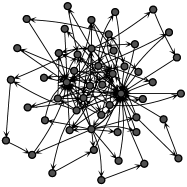
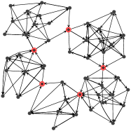
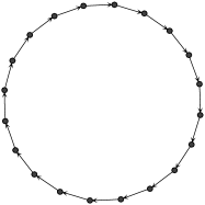
In principle, networks can respond in different ways to stochasticity in the update sequence (see Fig. 1): (a) The system has no specific sequence of states, and it quickly looses memory of its past states. (b) The system has some degree of ordering in the sequence of states, with “checkpoint” states that occur in a given order, and with certain groups of states occurring in between. (c) The system has entirely reliable dynamics, where the sequence of states is always the same on the attractor, no matter in which order the nodes are updated.

In this paper, we will focus on systems that have an attractor that has entirely reliable dynamics. Many cellular processes, such as the response to some external signal, or the cell cycle, can only function correctly if the system goes through the required sequence of states in the correct order. Therefore, considering the idealization of fully reliable dynamics is biologically motivated. Furthermore, studying networks with entirely reliable dynamics is also of theoretical interest, since it is an idealized situation on which one can build when studying more complicated cases. Entirely reliable dynamics can be implemented by enforcing that consecutive states of the attractor trajectory differ only in the value of one node. In other words, the Hamming distance between successor states is always 1. It is obvious that this is the only possible type of trajectory that can be entirely independent of the update schedule. If two subsequent states differed by the state of two or more nodes, then it would be possible to devise an update sequence which would update one node but not the other, in contradiction to our assumption.

Entirely reliable attractors are represented in state space as simple loops. We denote the number of different states on the attractor by $L=\sum_{i}l_{i}$, where $l_{i}$ is the number of times node $i$ changed its state during a full period (since the trajectory is periodic, $l_{i}$ must be equal to 0 or a multiple of 2). Furthermore, if the states of the system were represented by the corners of a $N$-dimensional Hamming hypercube, the trajectory should follow its edges (see Fig. 2). The shortest possible trajectory length, considering that no node remains at a constant value, is $L=2N$, with $l_{i}=2$ for all nodes. The longest possible trajectory length is $L=2^{N}$, where all states of the system are visited, and the trajectory corresponds to a Hamiltonian walk on the $N$-dimensional Hamming hypercube .

(a) Stochastic dynamics

(b) “Checkpoint” states

(c) Entirely reliable trajectory

Figure 1: (Color online) Ilustration of levels of dynamical reliability. Each node on the graphs above is a state of the system, and the edges represent possible transitions between them.

Figure 2: Example of reliable trajectory of length $6$ on a system of size $N=3$.

III Minimal reliable networks

III.1 Construction rule

The goal of this section is to construct BNs that have a given entirely reliable trajectory, and to investigate their properties. A fully reliable trajectory has the property that the sequence of states is independent of the updating scheme, which means that under parallel update only one node at a time changes its state. How networks that go through a given sequence of states can be constructed, was demonstrated by Lau et al Lau et al. (2006), who investigated all possible networks which exhibit the main trajectory of the Yeast cell cycle regulatory network. Thus, we first define the dynamics, from which we obtain the topology and functions, opposite to what is usually done in the literature on Boolean Networks.

In fact, there exist many networks that display a given trajectory. Even when the full state space structure is specified, which defines the successor state of each of its $2^{N}$ possible states, it is possible to construct a network that has this state space structure. This can be done by constructing a fully connected graph with $k=N$ and by assigning to each node the function that has the required output for each of the $2^{N}$ input states. In the end, inputs that never affect the output can be removed. If there are different sets of inputs that can be simultaneously removed, different networks are obtained.

When not the entire state space structure, but only one reliable trajectory is specified, there exist consequently many networks with different topology and functions which have this trajectory and may differ in the rest of their state space. We will restrict ourselves to minimal networks, i.e., networks with the smallest possible number of inputs for each node and the simplest possible functions, which have the maximum possible number of identical entries in the truth table. This minimality condition is motivated by the putative cost associated with more connections or more complicated functions, which would decrease the fitness of an organism. This is in contrast to what was done in Lau et al. (2006), where all possible networks were considered, which is only feasible on very small systems.

Such minimal networks can be constructed by a straightforward algorithm, because the inputs and the function required for each node can be determined independently from those of all the other nodes. The inputs for a given node must include all predecessor nodes, which change their state 1 time step before the given node changes its state. Additional inputs are required if the given node assumes, during the course of the trajectory, different binary states for the same configuration of the predecessor nodes. The choice of these “excess” inputs is usually not unique and may include self inputs. We perform this choice at random, but only from the possibilities which minimize the number of inputs to each node. If not all possible configurations of the states of the input nodes occur during the course of the trajectory, the update function of the given node is not unique. We first assign those truth table entries of the update function that are specified by the trajectory. Then, we assign to all remaining entries the same output value, and we choose the majority of output values assigned so far. (If there is no majority, we choose either value with probability 1/2.)

The algorithm used for choosing the minimal set of inputs proceeds as follows: To each node, we first assign all predecessor nodes as inputs. Then, if needed, we choose “excess” inputs. We first set the number of excess inputs to $k^{\prime}=1$, and we test in a random order the ${N\choose k^{\prime}}$ possible node combinations until we find a node set which, together with the predecessors, is a valid input set. If no valid combination is found, we increase $k^{\prime}$ by 1 and repeat the search. Once a valid combination is found, the corresponding truth table is completed by applying the minimality condition to its unspecified entries. The run time of this algorithm increases as $O(lN^{\max(\max(k^{\prime}),1)})$, where $l$ is the average number of flips per node, and $\max(k^{\prime})$ is the maximum value of $k^{\prime}$ for all nodes. We have observed that the run times are feasible for networks of size up to $N=400$ and $l=12$. 

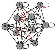
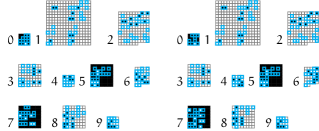
An example for a reliable trajectory and two possible networks with their functions, obtained with the above algorithm, is given in Figure 3.

Figure 3: (Color online) Example of a random reliable trajectory for $N=10$ and $l=4$, and two possible minimal networks. The edges with dashed (red) lines represent the inputs that are different between the two networks. Below each network are the outputs of the truth table of each node, ordered from top to bottom, and left to right, according to their input combination indices. Outputs marked in grey (cyan) correspond to input combinations present in the given trajectory.

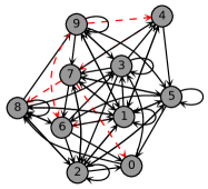
We choose the reliable trajectory at random, without taking into consideration possible particular features of biological networks, such as different temporal activation patterns of the different nodes, which reflect the function that the network must fulfill. Instead, we will consider a null model, where the values of the nodes change randomly. The only restriction which is imposed is that the trajectory is reliable. The only two parameters of this trajectory are the number of nodes $N$, and the average number of flips per node $l$. We generate a random ensemble of reliable trajectories in the following way: First, we determine how often each node shall be flipped. To this purpose, for each node $i$ a random number $\lambda_{i}$ is chosen from a Poisson distribution with mean $(l-2)/2$, implying that node $i$ shall be flipped $l_{i}\equiv 2\lambda_{i}+2$ times. The average number of flips of each node is thus identical to $l$, and each node is flipped at least twice. The length of the trajectory is then $L=2N+2\sum_{i}\lambda_{i}=\sum_{i}l_{i}$. Then, we arrange these flips in a randomly chosen order. If the resulting trajectory contains the same network state twice, it is discarded, and a new sequence of flips is chosen.

III.2 Topological characteristics

We first present results for the topological characteristics of the obtained networks. We evaluate the degree distribution and the local correlations. The degree distribution is of course strongly dependent on $l$. Local correlations can arise when two nodes that are influenced by the same nodes are more likely to influence each other.

Unless stated otherwise, we averaged the results from several independent realizations of the minimal trajectories and minimal networks, for different $N$ and $l$. The number of realizations for small $N$, up to $20$, were at least $2000$. For intermediary values of $N$, up to $100$, it varied from 50 to 300, depending on $l$. For the larger networks, $N>100$, it ranged from 200 to 6 networks for $l<12$, and one realization for $N=400$ and $l=12$.

III.2.1 Degree distribution

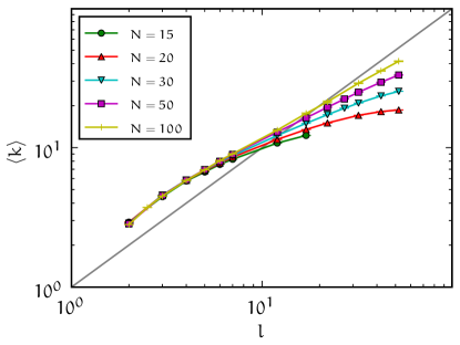
The number of inputs of a node is at least as large as the number of its predecessors. Whenever the state of the node cannot be written as a function of the predecessors alone, “excess” inputs must be chosen, as already mentioned before. The number of different predecessors $n_{p}$ per node approaches, for large $N$, on average $l$, since it becomes unlikely for large $N$ that the same node is chosen twice as predecessor. The typical truth table size grows therefore with $l$ as $2^{l}$. Since the number of different predecessor states grows only quadratically as $n_{p}l\sim l^{2}$, one can expect the number of “excess” inputs to be small, and number of inputs per node should be

$${\left<k\right>}\simeq l,$$ (2)

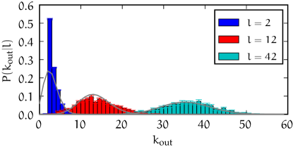
for sufficiently large $N$. This is confirmed by our numerical investigations, as is shown in Fig. 4.

Figure 4: (Color online) Average degree ${\left<k\right>}$ as function of $l$ for networks of different size $N$. The straight line is the function ${\left<k\right>}=l$.

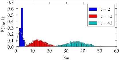
The degree distribution mirrors the distribution of the number of predecessors. Since all nodes flip on average the same number of times, the distribution is expected to follow a Poisson distribution for large enough $l$. This is indeed the case, as Fig. 5 shows. For small $l$ however, the distributions are more narrow, because we imposed the condition that each node flips at least twice, leaving little freedom for additional predecessors when $l$ is close to 2.

Figure 5: (Color online) In-degree and out-degree distributions of minimal networks for different values of $l$, for $N=100$. The solid lines correspond to Poisson distributions with the same average.

III.2.2 Local correlations

We obtained information about the local topology of the minimal networks by evaluating the probability that the neighbours of a given node are connected to each other. This probability is the so-called clustering coefficient ${\left<c\right>}$ Newman (2003). Random uncorrelated networks show absence of clustering only in the limit $N\to\infty$. Thus, for finite $N$, it is necessary to compare the obtained value with a random network of equal size and with equal degree distribution. In order to do this, we calculated the clustering coefficient ${\left<c_{s}\right>}$ on shuffled networks, where the links were rewired randomly, preserving the in- and out-degree of each node. We then calculated the ratio ${\left<c\right>}/{\left<c_{s}\right>}$, for networks of different size and average flip number $l$. If the ratio approaches $1$, the network does not exhibit any special clustering. The results for several values of $N$ and $l$ are shown in Fig. 6.

Figure 6: (Color online) Clustering ratio ${\left<c\right>}/{\left<c_{s}\right>}$ as a function of the average number of flips per node $l$, for different network sizes $N$. The gray straight line corresponds to a decay of the type $1/N$.

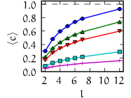
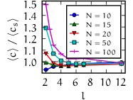
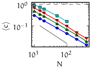
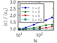
The most evident feature of Fig. 6 is that clustering is stronger for smaller $l$, i.e., for sparse networks. For larger $l$ (and hence larger ${\left<k\right>}$), the average distance between nodes decreases, and the shuffled and original networks have a similar degree of clustering. This difference between networks with smaller and larger average degree becomes more pronounced when the size of the networks $N$ is increased. From the data in Fig. 6, it appears that that the ratio ${\left<c\right>}/{\left<c_{s}\right>}$ increases slowly with $N$. We will argue in the following that this ratio will reach a finite asymptotic value in the limit $N\to\infty$.

The finding that the clustering coefficients are larger than for random networks can be explained by considering the above-mentioned excess inputs that are required when the function assigned to a node cannot be based on its predecessor nodes alone. Let us consider two consecutive flips of a node $j$ on a given trajectory. These flips are preceded by flips of the predecessor nodes, which we call $v$ and $w$. The average time between the two considered flips of node $j$ is $\sim L/l=N$, implying that there is a considerable probability that node $v$ flips again before the second flip of node $j$, giving the sequence

$$vj\cdots v\cdots wj\,.$$

The update function assigned to node $j$ needs an excess input if neither node $w$ nor any other predecessor of node $j$ (which can exist only for $l>2$) flips between the first flip of $j$ and the second flip of $v$. The simplest choice of this excess input is node $j$ itself. Indeed, self-inputs occur more often than in the shuffled networks, as is shown in Fig. 7. Since the number of different possible excess inputs is proportional to $N$, we expect that the fraction $n_{l}$ of nodes with self-inputs decreases as $n_{l}\sim 1/N$ for large $N$, but remains larger than that of shuffled networks by a constant multiplicative factor.

Figure 7: (Color online) Fraction $n_{l}$ of nodes with self-input, as a function of $N$, for different values of $l$. The dashed curves are obtained for shuffled networks, with the same degree sequence. The inset shows the ratio $n_{l}/n^{s}_{l}$, where $n^{s}_{l}$ is the self-input ratio for the shuffled networks.

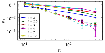
The excess input cannot be a self-input if node $w$ flips also in the same interval, giving the sequence

$$vj\cdots v\cdots w\cdots wj\,.$$

In this case, an excess input $u$ must be chosen among those nodes that flip between the two consecutive flips of node $w$, if none of the other predecessors of $j$ flips in this interval, giving the sequence

$$vj\cdots v\cdots w\cdots u\cdots wj\,.$$

Now, the average distance between the flips of node $w$ and node $u$ is smaller than that between two randomly chosen nodes, since $w$ is required to flip in the indicated interval. Therefore, the probability that $w$ is an input to $u$ or vice versa is larger than random, and it scales as $1/N$ in the limit $N\to\infty$. Since $w$ and $u$ are inputs to $j$, it follows that the clustering coefficient is larger than the random value ${\left<c_{s}\right>}$.

From this consideration, it follows that the ratio ${\left<c\right>}/{\left<c_{s}\right>}$ approaches a constant value in the limit $N\to\infty$. Furthermore, it follows that this ratio is larger for smaller $l$, since it is less likely that there exist additional inputs to $j$ that flip in the required interval and make excess inputs unnecessary. The slight increase seen in Fig. 6 can probably be attributed to a finite-size effect.

Figure 8: (Color online) The $z$-score of the different three-node subgraphs of minimal reliable networks, for different values of $l$ and $N=100$. The profile $z_{\text{st}}$ corresponds to the the signal-transduction interaction network in mammalian cells Milo et al. (2004).

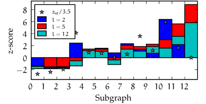
In order to determine which three-node subgraphs contribute to the increased clustering, we evaluated their $z$-score, which indicates to what extent the frequency of each subgraph is different compared to the random case. The $z$-score is defined as

$$z_{i}=\frac{{\left<N_{i}\right>}-{\left<N^{s}_{i}\right>}}{\sqrt{{\left<(N^{s}_{i})^{2}\right>}-{\left<N^{s}_{i}\right>}^{2}}},$$ (3)

where $N_{i}$ is the number of occurrences of subgraph $i$, and $N_{i}^{s}$ is the number of occurrences of the same subgraph on a shuffled network with the same degree sequence. Fig. 8 shows the different possible subgraphs and their $z$-score. Subgraphs with more links have a higher $z$-score and are therefore network motifs. Sparser subgraphs, where there is no link between two of the nodes, are rarer than at random, as predicted by the clustering coefficient. The abundance of denser motifs increases with $l$, as the network itself becomes more dense, but the overall trend of the $z$-score is the same. One peculiar feature is the absence of simple loops (subgraph 6), also know as feedback loops Alon (2007). As was described above, the clustering is mostly due to the correlations between the inputs of a given node. A simple loop does not have this type of correlation. Furthermore, it was shown by Klemm et al Klemm and Bornholdt (2005b) in a study of the reliability of small Boolean networks, that feedback loops are harmful to reliable dynamics. These authors obtained a $z$-score profile very similar to Fig. 8 (see Fig. 4 of Klemm and Bornholdt (2005b)). They also showed that this profile is qualitatively similar to real biological networks studied in Milo et al. (2004). A direct comparison is shown in Fig. 8, with the motif profile of the signal-transduction interaction network in mammalian cells Milo et al. (2004).

(a) $k=2$

(b) $k=3$

(c) $k=3$, without self-loops.

(d) $k=4$, without self-loops.

Figure 9: (Color online) Distribution of the different update functions, for different numbers of inputs, $k$, and for different flip numbers, $l$, for networks of size $N=20$.

In Fig 8, we did not keep track of the self-inputs, for simplicity. When self-loops are included in the subgraphs, their number increases from 13 to 86, which makes the analysis and presentation more elaborate. We performed this analysis and found that a subgraph with a specific number of self-loops has a larger $z$-score than its counterpart with less or no self-loops. The $z$-score pattern of Fig. 8, on the other hand, is repeated for subgraphs which share the same number of self-loops, which shows that motif occurrence and self-regulation are largely independent.

III.3 Properties of update functions

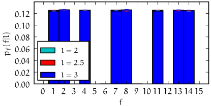
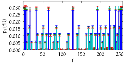
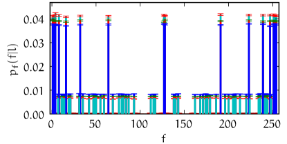
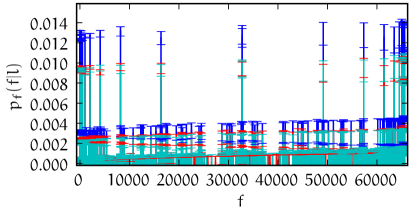
We evaluated the frequency of the different types of update functions in minimal networks, for different values of $l$, see Fig. 9. Unless otherwise stated, the results were obtained from $10^{4}$ independent realizations of networks with $N=20$. We compared the results with those obtained for larger values of $N$, with no discernible difference other than the reduced statistical quality. Functions with different numbers of inputs were evaluated separately.

The functions seem to be distributed according to different classes, where functions of the same type occur with the same probability, while some do not occur at all. In order to understand this distribution, it is necessary to describe in detail what conditions need to be met by the functions, according to the imposed dynamics and construction rules.

The subsystem composed only of the inputs of a given node follows a certain “local trajectory” (i.e., sequence of states), which determines, together the minimality condition described in Sec. III, the update function of the considered node. The probabilities of the different possible trajectories depend on the way the global trajectory is specified, and on the rules for choosing excess inputs. The restrictions imposed on the local trajectories of the inputs are as follows:

1. The local trajectory of the inputs must correspond to a periodic walk on the $k$-dimensional hypercube representing their states, since the Hamming distance at each step must be $1$. We note that in this subsystem, the same input state is allowed to repeat within a period (only the global state cannot). The vertices of the hypercube can be annotated with the output value of the function at the corresponding input state (see Fig. 10 for examples).

2. For large $N$, the trajectories of any two different nodes will be approximately random and uncorrelated. The only restriction is that every face of the hypercube will be visited exactly $l_{v}$ times, where $v$ is the index of the input node that has a fixed state on this face. On average we have ${\left<l_{v}\right>}=l$.

3. The output values of the function can be distributed on the vertices of the hypercube that are visited during the walk in any possible way, with the restriction that the output value must change $l_{j}$ times along the walk, where $j$ is the index of the considered node. An exception are functions with self-inputs: the vertices on the hypercube face corresponding to the self-input must all have the same output value.

4. The output values at the vertices of the hypercube which are not visited by the walk must be equal to the majority of the output values on the walk (this is the minimality condition defined in section III).

5. Functions that can be reduced to a function with smaller $k$ cannot occur due to the minimality condition, and the corresponding trajectory can be confined to a hypercube of smaller dimension.

Fig. 10 shows examples of trajectories that are allowed or not allowed for the case $k=3$.

(a) Valid trajectory

(b) Invalid (restriction 2)

(c) Invalid (restriction 4)

(d) Invalid (restriction 5)

Figure 10: Example of input and output trajectories on the $k$-hypercube representing the states of the inputs, for functions with $k=3$. Allowed transitions are represented by arrows. The color on each vertex represent the output value. Fig. (a) represents one type of valid trajectory. Figs. LABEL:sub@fig:traj_r2 to LABEL:sub@fig:traj_r4 represent invalid trajectories according to the indicated restriction: LABEL:sub@fig:traj_r2 not all sides of the cube are visited; LABEL:sub@fig:traj_r3 the function is not minimal; LABEL:sub@fig:traj_r4 the function can be reduced to $k=2$.

The listed restrictions result in the observed distribution of update functions. We will describe in detail all the possibilities for $k=2$, and discuss in a more general and approximate manner the functions with $k>2$.

III.3.1 Functions with $k=2$

Fig. 9 shows that only 8 of the 16 possible functions occur, and all of them with equal probability. They are all canalyzing functions, with three entries 1 (or 0) in the truth table, and one entry 0 (or 1). The hypercube representation of all functions is shown in Fig. 11. The functions that are not possible are obviously the constant functions (first row of Fig. 11, from left to right), and the functions which are insensitive to one of their inputs, due to restriction 4 (second and third row). The other functions which do not occur are the reversible functions, which change the output at every change of an input (fourth row). Those functions, however, are not entirely impossible: It is possible to construct a trajectory that meets all the listed requirements, with the specification that the output flips as often as all inputs together (restrictions 2 and 3). Such trajectories follow the pattern

$$vj\cdots wj\cdots vj\cdots wj,$$

where $v$ and $w$ are the inputs of $j$. This pattern is impossible for $l=2$, but can occur for larger $l$, albeit with a small probability, since $k=2$ functions are less likely for larger $l$; furthermore, the probability that a node has two predecessors which occur twice decreases with $N$ as $\sim 1/N^{2}$.

Figure 11: Representation of all 16 functions with $k=2$ on the 2-hypercube. On the left are the functions which do not (or rarely) occur in the minimal networks, and on the right are the canalysing functions which occur with equal probability.

III.3.2 Functions with $k>2$

Functions with $k>2$ seem to fall into different classes, which occur with different probabilities. This can be seen by plotting the distribution of the probabilities $p_{f}$ of the different functions, as shown in Fig. 12LABEL:sub@fig:all-classes for $k=5$. The different classes seem to correspond to different function homogeneity values, defined as the number of minority output values in the truth table, $d$. This can be verified by selecting only those functions with a given value of $d$, and plotting their distribution of probabilities, as shown in Figs 12LABEL:sub@fig:class-d1 to LABEL:sub@fig:class-d4. The most frequent class comprises the functions with only one entry in the truth table deviating from the others ($f=2^{i}$ and $f=2^{k}-2^{i}$), with $d=1$ (see Fig 12LABEL:sub@fig:class-d1). Those are canalysing functions, where all inputs are canalysing inputs. Functions with the same homogeneity fall into subclasses which have different probabilities. Those functions are often negated functions ($f^{\prime}=2^{k}-f$) of one another, and this is due to the existence of self-inputs: Self-regulated functions are not equivalent functionally when they are negated (the input corresponding its own output must be negated as well), despite sharing the same homogeneity. The $0\leftrightarrow 1$ symmetry, however, is always preserved. When self-loops are ignored, the distribution becomes symmetric with respect to negation of the output (see Fig 9LABEL:sub@fig:fhist-k3-nl), and the homogeneity classification becomes the predominant criterion to distinguish between the classes (compare Figs 12LABEL:sub@fig:all-classes and LABEL:sub@fig:all-classes-nl). But even in the absence of self-loops, the probability classes are not uniquely defined by the homogeneity, and there are overlaps between the different classes, as Figs 12LABEL:sub@fig:class-d2 to LABEL:sub@fig:class-d4 show. Nevertheless, there is a general tendency that functions with larger $d$ are less likely.

(a) All functions

(b) No self-loops

(c) $d=1$, no self-loops

(d) $d=2$, no self-loops

(e) $d=3$, no self-loops

(f) $d=4$, no self-loops

Figure 12: (Color online) Distribution of function weights $p_{f}$, subdivided according to the value of the truth table homogeneity $d$, for different values of the average flip number $l$, for fixed values $k=5$ and $N=20$.

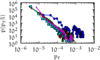
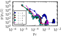
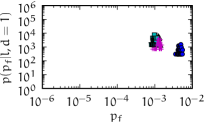
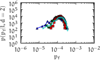
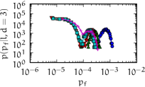
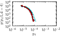
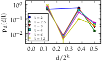
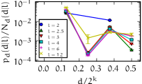
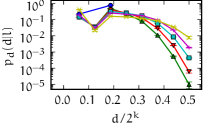
Fig. 13 shows the probability of finding a function with a given value of $d$. Since the number of different functions in a given class increases rapidly with $d$ for small $d$, the maximum of this distribution is shifted to values of $d$ larger than $1$. If this distribution is corrected by the number $N_{d}$ of different functions found with the same value of $d$, an overall decreasing function of $d$ is obtained, as shown in the graphs in the left column of Fig. 13).

(a) $k=3$

(b) $k=4$

(c) $k=6$

Figure 13: (Color online) Distribution of functions with different values of the truth table homogeneity $d$, for different average flip number $l$, and $N=20$.

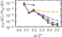
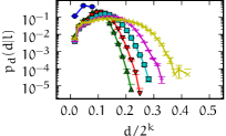
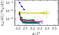
The observed difference in probability due to different homogeneity can be explained as follows. We consider a node with $k$ inputs. We denote by $M=\sum_{i}m_{i}\in[l/2,L-l/2]$ the total time during which the node is in the state that it assumes less often. The sum is taken over all intervals during which the node has this state.

If we denote the different possible (combined) states of the input nodes by letters, we can represent the sequence of states through which the considered node and its input states go by the following picture:

The shaded areas correspond to the output value 1. A state of the input nodes that appears inside the shaded (clear) area, must appear again inside the shaded (clear) area each time it is repeated. If we consider only the above scenario, and essentially ignore that the trajectories must follow the edges of a $k$-hypercube, we can show that functions with smaller values of $d$ should occur more often.

Our approximations rely on the fact that, for $N\to\infty$ and $l\gg 1$ (and hence $L\to\infty)$, the shaded areas will be more numerous and will be further apart in time and less correlated. In this limit, the input state number $i$ occurs, say, $n_{i}$ times. The probability that each of the input states occurs only in one type of area is given approximately by

$$\prod_{i}\left[\left(\frac{M}{L}\right)^{n_{i}}+\left(\frac{L-M}{L}\right)^{n_{i}}\right]\,.$$ (4)

The maximum of this function is attained at $M=l/2$ (or $M=L-l/2$, which is excluded since we chose $M$ such that it counts the minority part), which is the minimal possible value. The value of $d$ is bounded by $M$, but can be smaller since the same input state can repeat. We can in fact see that the case where the same state repeats at all $M$ times is more probable, by considering all the possible permutations of the state sequence, for a given value of $d$,

$$\left[\prod_{i\leq d}{M-\displaystyle\sum_{j<i}n_{j}\choose n_{i}}\right]\left[\prod_{i>d}{L-M-\displaystyle\sum_{d<j<i}n_{j}\choose n_{i}}\right]$$ (5)

and observing that it has a maximum at $d=1$, since $M\ll L$. (This means that there are $M$ shaded areas of size 1 each.) It follows that with increasing $l$ the weight of update functions with $d=1$ will become much larger than that of every other update function, as is evident from Figs. 9 and 13. The dominance of $d=1$ functions can already be seen for small values of $l$, although it is less pronounced.

III.4 State space structure

Finally, we investigated the state space of the constructed networks. We considered the system under a stochastic update scheme, since this scheme underlies the study presented in this paper. In this case, we define an attractor as a recurrent set of states in state space, with the property that there are no transitions that escape this set (i.e. a strongly connected component in the state space graph that has no outgoing connections). The number of states in this set is called the size of the attractor.

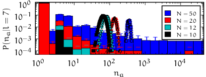
We evaluated the probabilities of attractors of a given size on the ensemble of minimal networks, and their average basin size. For small networks (up to $N=12$) the attractor size probability was obtained by exact enumeration of the state space. For larger $N$, the state space was sampled, taking care that the same attractor was not counted twice. This method, however, leads to a bias, since attractors with smaller basins are less likely to be counted, and the extent of this bias depends on the size of the network. Nevertheless, this bias is not relevant for our point of interest, which is on the occurrence of various attractors, but not on their precise statistics. Fig. 14 shows that there exist almost always fixed points, and that there are often attractors which are much larger than the imposed reliable trajectory (we considered attractors of up to $n_{a}=10^{5}$ states). Note that the probabilities in Fig. 14 do not sum to $1$, since a given network may have many attractors of different sizes.

Figure 14: (Color online) Probability of attractor sizes $n_{a}$, for $l=2$ and $l=7$. Attractors corresponding to the given trajectories are plotted separately with symbols. For each value of $N$ and $l$, $10^{4}$ different networks were analysed. In the case of attractor sampling, $100$ different random initial conditions per network were used.

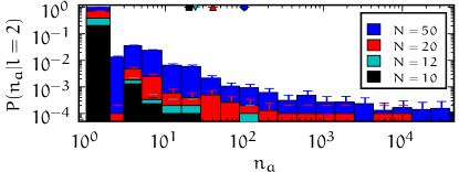
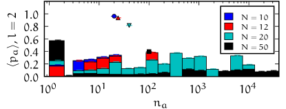
The basin of attraction was measured as the probability of reaching an attractor, starting from a random configuration. Fig. 15 shows that the omnipresent fixed point has a large basin of attraction. Larger attractors occur with smaller probabilities. The weight of the fixed point, compared to the weight of the imposed reliable trajectory, increases with increasing $N$. This can be explained by the entries in the truth table which are not uniquely determined by the reliable trajectory: While number of entries fixed throughout the trajectory grow linearly with $l$, the number of remaining entries (as well as their contribution to the state space) grow exponentially. In this increasingly large region of the state space, the functions behave as constant functions.

Figure 15: (Color online) Average attractor probabilities (basin size), $\left<p_{a}\right>$, for $l=2$ and $l=7$. Attractors corresponding to the given trajectories are plotted separately with symbols. For each value of $N$ and $l$, $10^{4}$ different networks were analysed, and $100$ different random initial conditions per network were used.

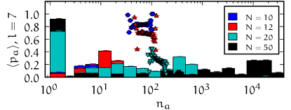
Attractors which are larger than the given trajectories are due to a portion of network begin frozen in the value they have at the fixed point, while other nodes remain frustrated, and their states change stochastically, visiting a larger portion of the state space, without entering the fixed point or the reliable trajectory.

For comparison, we briefly looked at the attractor sizes obtained using a synchronous updating scheme. Not surprisingly, the attractors become much shorter in this case, with attractors larger than the given trajectory having only a small probability (not shown).

IV Conclusion

We have constructed minimal Boolean networks which follow a given reliable trajectory in state space. The trajectories considered have the necessary feature that only one node can change its value at any moment in time, which guarantees that the sequence of states is independent of the order in which nodes are updated. Otherwise the nodes change their states at randomly assigned times in the given trajectory, thus constituting a null model for reliable dynamics. The minimality condition imposed on the networks was that it contains the smallest possible set of inputs for each node that allows for the given trajectory. Additionally, the truth table entries that are not fixed by the trajectory were set to the majority value imposed by the trajectory. We then investigated the topology, the update functions, and the state space of those networks.

The network structure, as manifest in the degree distribution, does not deviate significantly from a random topology. However, the network exhibits larger clustering than a random network, and exhibits a characteristic motif profile, which resembles both real networks of gene regulation and the pattern of dynamically reliable motifs found in Klemm and Bornholdt (2005b). The existence of clustering and motifs was explained by considering the “excess” inputs that are required to avoid contradictions in the truth table, and how they must be correlated among each other.

The update functions of the nodes show a characteristic distribution, where only a subset of the possible functions occur, and these are divided into distinct classes, which occur with different probabilities. The main factor discerning the different classes is their homogeneity, characterized by the number of entries of the minority bit in the truth table. Function with homogeneity 1 occur with increased probability, and become the dominant functions in the limit of large trajectories, $l\to\infty$, for fixed $k$. Functions with more minority entries occur with a smaller probability, and this probability decreases as the number of minority entries increase. We presented an analytical justification for this finding, considering how the local trajectory of the input states of a given function must behave, in the limit $l\gg 1$.

Finally we investigated the state space of the constructed networks, considering the possible attractors it can have, in addition to the given reliable trajectory. To this aim, we used a stochastic update scheme. We observed that the network almost always exhibits a fix point of the dynamics, and often attractors which can be much larger than the given trajectory. The basin size of the fixed point is very large, and dominates the basin size of the given trajectory in the limit of large system size. This is a consequence of the minimality condition imposed on the network: The region of state space dictated by the imposed trajectory increases only linearly with system size, while the entire state space grows exponentially. Outside the state space region fixed by the reliable trajectory, the constructed functions behave as constant functions, which drive the system nearer to the frozen phase.

In this work, we have used a null model for reliable trajectories, where the nodes change their values at random times. Real gene regulatory networks deviate significantly from this, since they must agree with the cell cycle or the pathway taken during embryonic development. Certain proteins need to be always present in the cell, while others are produced only under specific conditions. The degree distribution and the update functions must reflect this behavior. However, some of the features found for the null model presented in this work, should also be present in more realistic systems. The existence of clustering, and the motif profile found, for instance, do not depend strongly on the specific temporal patterns of the nodes, but are imposed by the reliability condition. Similarly, the dominance of strongly canalyzing functions is a consequence of the reliability condition and should be relatively robust to the introduction of temporal correlations. Nevertheless, biochemistry makes some canalyzing functions more likely than others.

An important feature of biological networks that is not reflected in the null model presented in this paper, is the robustness with respect to perturbations of a node. Such a robustness can only be obtained when more than the minimum possible number of inputs is assigned to a node. Indeed, it has been shown in Gershenson et al. (2006) that more redundancy allows for more robustness. Similarly, requiring that the reliable trajectory has the largest basin of attraction or that other attractors of the system are also reliable trajectories, may increase the number of links in the network.

Finally, the requirement that trajectories are fully reliable is an idealization which goes beyond what is necessary for gene regulatory networks. Real networks have checkpoint states, but between these states, the precise sequence of events is not always important. On the other hand, full reliability may be necessary for certain subsystems of the gene network, where a strict sequence of local states is required. The minimal reliable networks discussed in this paper should be compared more realistically to such reliable modules.

V Acknowledgements

We thank Ron Milo for providing the signal-transduction network data. We acknowledge the support of this work by the Humboldt Foundation and by the DFG under contract number Dr300/5-1.

References

- Rosen-Zvi et al. (2001) M. Rosen-Zvi, A. Engel, and I. Kanter, Phys. Rev. Lett. 87, 078101 (2001).
- Moreira et al. (2004) A. A. Moreira, A. Mathur, D. Diermeier, and L. A. N. Amaral, Proc. Nat. Ac. Sci. 101, 12085 (2004).
- Lagomarsino et al. (2005) M. C. Lagomarsino, P. Jona, and B. Bassetti, Phys. Rev. Lett. 95, 158701 (2005).
- Wolfram (2002) S. Wolfram, A New Kind of Science (Wolfram Media, 2002), ISBN 1579550088.
- Kauffman (1969) S. A. Kauffman, J. Theor. Biol. 22, 437 (1969).
- Drossel (2008) B. Drossel, in Reviews of Nonlinear Dynamics and Complexity, edited by H. G. Schuster (Wiley, 2008), vol. 1.
- Greil and Drossel (2005) F. Greil and B. Drossel, Phys. Rev. Lett. 95, 048701 (2005).
- Klemm and Bornholdt (2005a) K. Klemm and S. Bornholdt, Physical Review E 72, 055101 (2005a).
- Li et al. (2004) F. Li, T. Long, Y. Lu, Q. Ouyang, and C. Tang, Proc. Nat. Ac. Sci. p. 0305937101 (2004).
- Lau et al. (2006) K. Y. Lau, S. Ganguli, and C. Tang, Mol. Syst. Biol Phys Rev E 75, 051907 (2006).
- Newman (2003) M. E. J. Newman, SIAM Review 45, 167 (2003).
- Alon (2007) U. Alon, An introduction to systems biology: design principles of biological circuits (Chapman & Hall/CRC, 2007).
- Klemm and Bornholdt (2005b) K. Klemm and S. Bornholdt, Proc. Nat. Ac. Sci. 102, 18414 (2005b).
- Milo et al. (2004) R. Milo, S. Itzkovitz, N. Kashtan, R. Levitt, S. Shen-Orr, I. Ayzenshtat, M. Sheffer, and U. Alon, Science 303, 1538 (2004).
- Gershenson et al. (2006) C. Gershenson, S. A. Kauffman, and I. Shmulevich, in Artificial Life X, Proceedings of the Tenth International Conference on the Simulation and Synthesis of Living Systems, edited by L. S. Yaeger, M. A. Bedau, D. Floreano, R. L. Goldstone, and A. Vespignani (MIT Press, 2006), pp. 35–42.
- Knuth (2005) D. E. Knuth, The Art of Computer Programming, Volume 4, Fascicle 3: Generating All Combinations and Partitions (Addison-Wesley Professional, 2005).