On the phase-integral method for the radial Dirac equation

Abstract

In the application of potential models, the use of the Dirac equation in central potentials remains of phenomenological interest. The associated set of decoupled second-order ordinary differential equations is here studied by exploiting the phase-integral technique, following the work of Fröman and Fröman that provides a powerful tool in ordinary quantum mechanics. For various choices of the scalar and vector parts of the potential, the phase-integral formulae are derived and discussed, jointly with formulae for the evaluation of Stokes and anti-Stokes lines. A criterion for choosing the base function in the phase-integral method is also obtained, and tested numerically. The case of scalar confinement is then found to be more tractable.

I Introduction

Several problems of interest in theoretical physics lead eventually to the differential equation

$$\left({d^{2}\over dz^{2}}+R(z)\right)\psi(z)=0,$$ (1)

where $R$ is a single-valued analytic function of the complex variable $z$. The form of (1.1) suggests looking for solutions expressed through a prefactor $A(z)$ and a phase $w(r)$, i.e.

$$\psi_{\pm}(z)=A(z)e^{\pm iw(z)}.$$ (2)

The Wronskian of $\psi_{+}(z)$ and $\psi_{-}(z)$ is equal to $-2iA^{2}{dw\over dz}$, and on the other hand the Wronskian of two linearly independent solutions of Eq. (1.1) is a constant. Thus, the prefactor $A(z)$ reads as const. $\times{1\over\sqrt{dw/dz}}$, and one has Froman02

$$\psi(z)={1\over\sqrt{q(z)}}e^{\pm iw(z)},$$ (3)

where

$$w(z)=\int^{z}q(\zeta)d\zeta,$$ (4)

the function $w$ being the phase integral, while $q$ is called the phase integrand. Moreover, upon insertion of the exact solution (1.3), (1.4) into Eq. (1.1), one finds that the phase integrand $q(z)$ should satisfy the $q$-equation

$$f(z,q(z),R(z))\equiv q^{-{3\over 2}}{d^{2}\over dz^{2}}q^{-{1\over 2}}+{R(z)\over q^{2}}-1=0.$$ (5)

In practice, however, the task of finding exact solutions of Eq. (1.5) is rather difficult. The best one can do is often to determine a function $Q$ that is an approximate solution of the $q$-equation (1.5), so that

$$\varepsilon_{0}\equiv f(z,Q(z),R(z))<<1.$$ (6)

The approximate phase-integral method consists in finding approximate solutions of Eq. (1.1) with unspecified base function $Q$. A criterion for finding $Q$ is that the function $\varepsilon_{0}$ defined in (1.6) should be much smaller than unity in the region of the complex-$z$ plane relevant for the problem. However, this criterion does not determine the base function $Q$ uniquely, the physicist has a whole set of basis functions $Q$ at his disposal, and this arbitrariness can be exploited.

On the other hand, along the years, many efforts have been devoted in the literature to the theoretical investigation of light fermions confined by a potential field PHRVA-D51-5079 . In the phenomenological applications, when dealing with mesons consisting of a heavy quark and a light quark, one can imagine that the heavy quark is indeed very heavy and acts as a “classical” source that can be represented as a superposition of Coulomb-like plus linear potential, better known as Cornell potential Cornell . The mass occurring in the Dirac equation is therefore the mass of the light quark. It is by now well known that, on using the Dirac equation, only Lorentz scalar confinement leads to normalizable stationary states, while in a suitable variant of the Dirac equation, called “no pair”, only Lorentz vector confinement has normal Regge behaviour. Hereafter we focus on the stationary Dirac equation for a quark of mass $m$ in a Lorentz scalar potential $V_{S}(r)$ and in the time component of a Lorentz vector potential $V_{V}(r)$, i.e. PHSTB-77-065005

$${dF\over dr}=-{\kappa\over r}F+{mc^{2}+E+V_{S}-V_{V}\over{\hbar}c}G,$$ (7)

$${dG\over dr}={\kappa\over r}G+{mc^{2}-E+V_{S}+V_{V}\over{\hbar}c}F,$$ (8)

where $\kappa=-l-1$ if $j=l+{1\over 2},\;\kappa=l$ if $j=l-{1\over 2}$. In the resulting second-order equations, first derivatives can be removed by putting

$$\begin{pmatrix}F(r)\\ G(r)\end{pmatrix}=\begin{pmatrix}\sqrt{E+mc^{2}+V_{S}-V_{V}}\hfill&0\\ \;\;\;\;\;\;\;0&\sqrt{E-mc^{2}-V_{S}-V_{V}}\end{pmatrix}\begin{pmatrix}f(r)\\ g(r)\end{pmatrix}.$$ (9)

Section II studies the second-order equations resulting from the radial Dirac equations (1.7) and (1.8), preparing the ground for the application of the phase-integral method. Section III describes various possible choices of basis function in the phase-integral method. Sec. IV arrives at a general criterion for choosing a suitable basis function $Q$. Sec. V performs a numerical analysis of the applicability of such a criterion. Sec. VI studies Stokes and anti-Stokes lines for the squared Dirac equation in a central potential, inspired by the choice of $Q$ made in the simpler analysis of central potentials in ordinary quantum mechanics. Concluding remarks and open problems are presented in Sec. VII.

II Second-order equations from the Radial Dirac equation

With the notation in the Introduction, our starting point is the following set of decoupled second-order equations obtained from the radial Dirac equation:

$$\begin{pmatrix}\frac{d^{2}}{dr^{2}}+R_{f}(r)\hfill&0\\ \;\;\;\;\;\;\;0\hfill&\frac{d^{2}}{dr^{2}}+R_{g}(r)\hfill\end{pmatrix}\begin{pmatrix}f(r)\\ g(r)\hfill\end{pmatrix}=0,$$ (10)

where the “potential” terms read as PHSTB-77-065005

$$R_{f}(r) \equiv {(E-V_{V})^{2}-(mc^{2}+V_{S})^{2}\over({\hbar c})^{2}}-{\kappa(\kappa+1)\over r^{2}}$$ (11)

$$+ \left[V_{V}^{\prime}-V_{S}^{\prime}\over mc^{2}+E+V_{S}-V_{V}\right]{\kappa\over r}-{(V_{V}^{\prime\prime}-V_{S}^{\prime\prime})\over 2[mc^{2}+E+V_{S}-V_{V}]}$$

$$- {3\over 4}\left[V_{V}^{\prime}-V_{S}^{\prime}\over mc^{2}+E+V_{S}-V_{V}\right]^{2},$$

$$R_{g}(r) \equiv {(E-V_{V})^{2}-(mc^{2}+V_{S})^{2}\over({\hbar c})^{2}}-{\kappa(\kappa-1)\over r^{2}}$$ (12)

$$+ \left[V_{V}^{\prime}+V_{S}^{\prime}\over mc^{2}-E+V_{S}+V_{V}\right]{\kappa\over r}-{(V_{V}^{\prime\prime}+V_{S}^{\prime\prime})\over 2[mc^{2}-E+V_{S}+V_{V}]}$$

$$- {3\over 4}\left[V_{V}^{\prime}+V_{S}^{\prime}\over mc^{2}-E+V_{S}+V_{V}\right]^{2}.$$

Note that, for energies $E<-mc^{2}$, the following difficulty arises: the relation between $f(r)$ and $F(r)$ in (1.9) becomes singular at the point $r=r_{f}$ such that $V_{V}(r_{f})-V_{S}(r_{f})=E+mc^{2}$. Thus, the effective potential $R_{f}(r)$ in (2.2) becomes infinite at $r\rightarrow r_{f}$. The solutions become meaningless near the point $r=r_{f}$ because the phase integrals diverge. Similar remarks Popov ; Zeldovich ; Lazur hold for $g(r)$ and the effective potential in (2.3). However, this difficulty is purely formal because the original Dirac system (1.7) and (1.8) is not singular at the point $r=r_{f}$. A powerful JWKB analysis of the first-order Dirac system (1.7) and (1.8) can be found in Lazur .

Equations (2.1)–(2.3) suggest exploiting the known properties of the differential equation (1.1), which, as we said, is much studied in classical mathematical physics and ordinary quantum mechanics. The change of dependent and independent variable that preserves the form of (1.1) without first derivative is given by

$$\psi(z)\equiv{1\over\sqrt{Q(z)}}\varphi(z),$$ (13)

$$w(z)\equiv\int^{z}Q(\zeta)d\zeta,$$ (14)

where the function $Q$ is not specified for the time being but will be suitably chosen later.

Upon defining

$$\varepsilon\equiv{R\over Q^{2}}-1+Q^{-3/2}{d^{2}\over dz^{2}}(Q^{-1/2}),$$ (15)

equation (1.1) can be expressed in the equivalent form

$$\left[{d^{2}\over dw^{2}}+(1+\varepsilon)\right]\varphi(w)=0.$$ (16)

Equation (2.7) is more convenient because it can be turned into a system of two linear differential equations of the first order. For this purpose, one assumes that the complex $w$-plane is cut in such a way that the functions appearing are all single-valued and $\varphi$ can read as

$$\varphi(w)=a_{1}(w)e^{iw}+a_{2}(w)e^{-iw}.$$ (17)

If we further impose that

$$a_{1}^{\prime}(w)e^{iw}+a_{2}^{\prime}(w)e^{-iw}=0,$$ (18)

the first derivative of $\varphi$ reduces to

$${d\varphi\over dw}=ia_{1}e^{iw}-ia_{2}e^{-iw},$$ (19)

and one obtains the desired system of two first-order ordinary differential equations, i.e. Froman65

$${da_{1}\over dw}={i\over 2}\varepsilon\Bigr{(}a_{1}+a_{2}e^{-2iw}\Bigr{)},$$ (20)

$${da_{2}\over dw}=-{i\over 2}\varepsilon\Bigr{(}a_{2}+a_{1}e^{2iw}\Bigr{)}.$$ (21)

Such a system can be written in matrix form as

$${da\over dw}=M(w)a,$$ (22)

having set

$$M(w)\equiv{i\over 2}\varepsilon\begin{pmatrix}1\hfill&e^{-2iw}\\ -e^{2iw}\hfill&-1\hfill\end{pmatrix},$$ (23)

$$a(w)=\begin{pmatrix}a_{1}(w)\\ a_{2}(w)\hfill\end{pmatrix}.$$ (24)

At this stage, one can replace the differential equation (2.13) by the integral equation

$$a(w)=a(w_{0})+\int_{w_{0}}^{w}M(w_{1})a(w_{1})dw_{1},$$ (25)

which can be solved by iteration, starting from the solution formula

$$a(w)=F(w,w_{0})a(w_{0}),$$ (26)

where

$$F(w,w_{0}) = 1+\int_{w_{0}}^{w}dw_{1}M(w_{1})+\int_{w_{0}}^{w}dw_{1}M(w_{1})\int_{w_{0}}^{w_{1}}dw_{2}M(w_{2})$$ (27)

$$+ \int_{w_{0}}^{w}dw_{1}M(w_{1})\int_{w_{0}}^{w_{1}}dw_{2}M(w_{2})\int_{w_{0}}^{w_{2}}dw_{3}M(w_{3})+...$$

Under the assumption that

$$\sum_{j}|M_{ij}(w)|\leq m(w),$$ (28)

where $m(w)$ is a non-negative quantity, one finds that, in any region of the complex-$w$ plane where the integral $\int_{w_{0}}^{w}m(w_{1})dw_{1}$ is bounded, the series in (2.18) is absolutely and uniformly convergent. From (2.4), the original equation (1.1) is then solved by

$$\psi(z)=a_{1}{e^{iw(z)}\over\sqrt{Q(z)}}+a_{2}{e^{-iw(z)}\over\sqrt{Q(z)}}=a_{1}(z)f_{1}(z)+a_{2}(z)f_{2}(z),$$ (29)

where

$$f_{1}(z)\equiv{1\over\sqrt{Q(z)}}e^{iw(z)},\;f_{2}(z)\equiv{1\over\sqrt{Q(z)}}e^{-iw(z)}.$$ (30)

Our main source on this topic, ref. Froman65 , contains all details about useful approximate formulae for the $F$-matrix and many peculiar properties of the phase-integral approximation, which should not be confused with the JWKB method Froman02 .

III Choice of the base function

The function $Q$ in Sec. II need not coincide, when squared up, with the function $R$ in Eq. (1.1). A guiding principle in the choice of base function is as follows: first find the pole of higher order (if any) in $R(z)$, and then choose $Q(z)$ in such a way that it cancels exactly such a pole (see below).

III.1 Scalar confinement

For example, the scalar confinement is achieved with the potentials PHRVA-D51-5079

$$V_{S}=ar,\;V_{V}=0,$$ (31)

for which the “potential terms” $R_{f}$ and $R_{g}$ in (2.2) and (2.3) reduce to

$$R_{f}={E^{2}-(mc^{2}+ar)^{2}\over({\hbar}c)^{2}}-{\kappa(\kappa+1)\over r^{2}}-{a\over(mc^{2}+E+ar)}{\kappa\over r}-{3\over 4}{a^{2}\over(mc^{2}+E+ar)^{2}},$$ (32)

$$R_{g}={E^{2}-(mc^{2}+ar)^{2}\over({\hbar}c)^{2}}-{\kappa(\kappa-1)\over r^{2}}+{a\over(mc^{2}-E+ar)}{\kappa\over r}-{3\over 4}{a^{2}\over(mc^{2}-E+ar)^{2}}.$$ (33)

The experience gained in ordinary quantum mechanics suggests therefore choosing Froman65

$$Q_{f}^{2}\equiv R_{f}+{\kappa(\kappa+1)\over r^{2}},$$ (34)

$$Q_{g}^{2}\equiv R_{g}+{\kappa(\kappa-1)\over r^{2}}.$$ (35)

III.2 Logarithmic potential

More generally, however, bearing in mind that singularities in (2.2) and (2.3) might receive a further contribution from $V_{V}$ or $V_{S}$ if they were of logarithmic type, one can take

$$V_{S}={1\over a}\log\left({r\over r_{0}}\right),\;V_{V}=0,$$ (36)

bearing also in mind that only a scalar potential is able to confine a quark in the Dirac equation, and that a relativistic $Q{\overline{q}}$ system is indeed well described by the choice (3.6), as shown in PHLTA-B97-143 . The potential terms $R_{f}$ and $R_{g}$ in (2.2) and (2.3) are then found to develop also a logarithmic singularity at $r=0$, because the l’Hospital rule for taking limits implies that

$$\lim_{r\to 0}{1\over r^{2}\log(r)}=\lim_{r\to 0}{1\over r^{2}\log^{2}(r)}=\infty.$$

We are then led to get rid of both the pole-like and logarithmic singularities of $Q$ at $r=0$, by defining

$$Q_{f}^{2}\equiv R_{f}+{\kappa(\kappa+1)\over r^{2}}+{\left(\kappa+{1\over 2}\right)\over r^{2}\log(r/r_{0})}+{3\over 4r^{2}}{1\over\log^{2}(r/r_{0})},$$ (37)

$$Q_{g}^{2}\equiv R_{g}+{\kappa(\kappa-1)\over r^{2}}-{\left(\kappa+{1\over 2}\right)\over r^{2}\log(r/r_{0})}+{3\over 4r^{2}}{1\over\log^{2}(r/r_{0})}.$$ (38)

Interestingly, we are suggesting a novel perspective on the logarithmic potential, arriving at it from the point of view of the singularity structure of the base function in the phase-integral method.

III.3 A linear plus Coulomb-type potential

One can also consider the Cornell potential Cornell which is linear in the scalar part and of Coulomb-type in the vector part, i.e.

$$V_{S}=ar,\;V_{V}={b\over r}.$$ (39)

As $r\rightarrow 0$, the centrifugal term ${\kappa(\kappa\pm 1)\over r^{2}}$ in $R_{f}$ (respectively $R_{g}$) is then found to receive further contributions with a second-order pole at the origin, so that we can remove such a singularity in $Q$ by defining

$$Q_{f}^{2}\equiv R_{f}+{\left[\kappa^{2}-{1\over 4}-(b/{\hbar}c)^{2}\right]\over r^{2}},$$

$$Q_{g}^{2}\equiv R_{g}+{\left[\kappa^{2}+{7\over 4}-(b/{\hbar}c)^{2}\right]\over r^{2}}.$$

However, the resulting integral (2.5) for the independent variable $w$ is too complicated for analytic or numerical purposes.

III.4 Analogy with central potentials in ordinary quantum mechanics

It is therefore more convenient, in our relativistic problem, to fully exploit the arbitrariness of the base function $Q$ by defining it in such a way that it coincides with the form taken by $Q$ in non-relativistic problems in a central potential. For example, for the Schrödinger equation in a central potential it is helpful to deal with a $Q$ function of the form Froman65 $Q^{2}=1+{2\eta\over r}$. In our problem, both $R_{f}$ in (2.2) and $R_{g}$ in (2.3) contain exactly, i.e. without making any expansion, the term $-{2Eb\over({\hbar}c)^{2}}{1\over r}$, which is indeed of the form ${2\eta\over r}$ with

$$\eta\equiv-{Eb\over({\hbar}c)^{2}}.$$ (40)

We thus look for

$$Q_{f}^{2}(r)=R_{f}(r)+u_{f}(r)=1+{2\eta\over r}.$$ (41)

In this equation, the desired additional term can be obtained in exact form as

$$u_{f}(r)=1+{2\eta\over r}-R_{f}(r),$$

where $R_{f}$ leads to exact cancellation of the terms proportional to ${1\over r}$. We then find, from (2.5) and (3.11) (see Froman65 ),

$$w_{f}(r)=2\eta\left\{\sqrt{{r\over 2\eta}\left(1+{r\over 2\eta}\right)}+\log\left[\sqrt{{r\over 2\eta}}+\sqrt{1+{r\over 2\eta}}\right]\right\},$$ (42)

and, from (2.6),

$$\varepsilon_{f}={R_{f}\over Q_{f}^{2}}-1+Q_{f}^{-{3\over 2}}{d^{2}\over dr^{2}}Q_{f}^{-{1\over 2}}={R_{f}\over Q_{f}^{2}}-1-Q_{f}^{-{1\over 2}}{d^{2}\over dw^{2}}Q_{f}^{1\over 2},$$ (43)

which yield, by virtue of (2.21),

$$f(r)=a_{1,f}{e^{iw_{f}(r)}\over\sqrt{Q_{f}(r)}}+a_{2,f}{e^{-iw_{f}(r)}\over\sqrt{Q_{f}(r)}},$$ (44)

where the functions $a_{1,f}$ and $a_{2,f}$ can be obtained from (2.13)–(2.18), with $\varepsilon=\varepsilon_{f}$ in (2.14).

By following an analogous procedure, we find

$$Q_{g}^{2}(r)=R_{g}(r)+u_{g}(r)=1+{2\eta\over r}=Q_{f}^{2}(r),$$ (45)

$$w_{g}(r)=w_{f}(r),$$ (46)

$$\varepsilon_{g}={R_{g}\over Q_{g}^{2}}-1+Q_{g}^{-{3\over 2}}{d^{2}\over dr^{2}}Q_{g}^{-{1\over 2}}={R_{g}\over Q_{g}^{2}}-1-Q_{g}^{-{1\over 2}}{d^{2}\over dw^{2}}Q_{g}^{1\over 2},$$ (47)

$$g(r)=a_{1,g}{e^{iw_{g}(r)}\over\sqrt{Q_{g}(r)}}+a_{2,g}{e^{-iw_{g}(r)}\over\sqrt{Q_{g}(r)}},$$ (48)

bearing in mind that $R_{g}\not=R_{f}\Longrightarrow\varepsilon_{g}\not=\varepsilon_{f}$, and setting now $\varepsilon=\varepsilon_{g}$ in (2.14) for the evaluation of $a_{1,g}$ and $a_{2,g}$.

We should now recall that, by virtue of the identity Froman65

$$M(w_{1})M(w_{2})...M(w_{n})$$ (49)

$$= \left({i\over 2}\right)^{n}\varepsilon(w_{1})\varepsilon(w_{2})...\varepsilon(w_{n})\left[1-e^{-2i(w_{1}-w_{2})}\right]\left[1-e^{-2i(w_{2}-w_{3})}\right]$$

$$... \left[1-e^{-2i(w_{n-1}-w_{n})}\right]\begin{pmatrix}1\hfill&e^{-2iw_{n}}\\ -e^{2iw_{1}}\hfill&-e^{2i(w_{1}-w_{n})}\end{pmatrix},$$

the $F$-matrix in (2.17)-(2.18) can be expressed through a fairly simple series, i.e. Froman65

$$F_{11}(w,w_{0})=1+\int_{w_{0}}^{w}dw_{1}\;{i\over 2}\varepsilon(w_{1})$$ (50)

$$+ \int_{w_{0}}^{w}dw_{1}\;{i\over 2}\varepsilon(w_{1})\int_{w_{0}}^{w_{1}}dw_{2}\;{i\over 2}\varepsilon(w_{2})\left[1-e^{-2i(w_{1}-w_{2})}\right]$$

$$+ ...,$$

$$F_{12}(w,w_{0})=\int_{w_{0}}^{w}dw_{1}\;{i\over 2}\varepsilon(w_{1})e^{-2iw_{1}}$$ (51)

$$+ \int_{w_{0}}^{w}dw_{1}\;{i\over 2}\varepsilon(w_{1})\int_{w_{0}}^{w_{1}}dw_{2}\;{i\over 2}\varepsilon(w_{2})\left[1-e^{-2i(w_{1}-w_{2})}\right]e^{-2iw_{2}}$$

$$+ ...,$$

$$F_{21}(w,w_{0})=-\int_{w_{0}}^{w}dw_{1}\;{i\over 2}\varepsilon(w_{1})e^{2iw_{1}}$$ (52)

$$- \int_{w_{0}}^{w}dw_{1}\;{i\over 2}\varepsilon(w_{1})e^{2iw_{1}}\int_{w_{0}}^{w_{1}}dw_{2}\;{i\over 2}\varepsilon(w_{2})\left[1-e^{-2i(w_{1}-w_{2})}\right]$$

$$+ ...,$$

$$F_{22}(w,w_{0})=1-\int_{w_{0}}^{w}dw_{1}\;{i\over 2}\varepsilon(w_{1})$$ (53)

$$- \int_{w_{0}}^{w}dw_{1}\;{i\over 2}\varepsilon(w_{1})\int_{w_{0}}^{w_{1}}dw_{2}\;{i\over 2}\varepsilon(w_{2})\left[1-e^{-2i(w_{1}-w_{2})}\right]e^{2i(w_{1}-w_{2})}$$

$$+ ...\;.$$

IV A general criterion for choosing the base function

We have also tried to find a base function Q by assuming its behaviour for small and large values of r, i.e.

$$Q(r)=\frac{\alpha_{1}}{r}+\alpha_{2}+\alpha_{3}r\,.$$ (54)

This base function can be analytically integrated, thus, in principle, we can obtain the phase integral according to (2.5). To fix the free parameter entering the previous expression we assume that the $\varepsilon$ parameter in (2.6) should vanish at small and large distances. However, this criterion does not ensure that $\varepsilon$ remains small throughout the whole range of values of $r$, and we have instead found regions where the resulting $\varepsilon$ is, regrettably, larger than $1$, thus making our choices unsuitable. A general method is instead as follows. Since we have to fulfill the condition (1.6) with $\varepsilon$ defined as in (2.6) and $R=R_{f}$ or $R_{g}$, we re-express (1.6) in the form

$$\left|R-Q^{2}+Q^{1/2}{d^{2}\over dz^{2}}(Q^{-1/2})\right|<<Q^{2},$$ (55)

and define

$${\cal A}\equiv R-Q^{2},$$ (56)

$${\cal B}\equiv Q^{1/2}{d^{2}\over dz^{2}}(Q^{-1/2}),$$ (57)

or, the other way around,

$${\cal A}\equiv Q^{1/2}{d^{2}\over dz^{2}}(Q^{-1/2}),$$ (58)

$${\cal B}\equiv R-Q^{2},$$ (59)

bearing in mind that

$$\left|\!\frac{}{}|{\cal A}|-|{\cal B}|\right|\leq|{\cal A}+{\cal B}|\leq|{\cal A}|+|{\cal B}|.$$ (60)

Moreover, we can always make the conventional choice according to which $|{\cal A}|>|{\cal B}|$.

When (4.3) and (4.4) hold, if both ${\cal A}$ and ${\cal B}$ are positive, the conditions (1.6) and (2.6) yield

$$R-Q^{2}+Q^{1/2}{d^{2}\over dz^{2}}(Q^{-1/2})\leq Q^{2},$$ (61)

i.e.

$$R-2Q^{2}+Q^{1/2}{d^{2}\over dz^{2}}(Q^{-1/2})\leq 0.$$ (62)

When (4.3) and (4.4) hold, if ${\cal A}>0$ and ${\cal B}<0$, conditions (1.6) and (2.6) yield

$$|R-Q^{2}|-\left|Q^{1/2}{d^{2}\over dz^{2}}(Q^{-1/2})\right|\leq Q^{2},$$ (63)

which coincides with (4.9) because ${\cal A}=R-Q^{2}>0$ while ${\cal B}=-|{\cal B}|<0$.

Nothing changes if instead (4.5) and (4.6) hold. For example, if ${\cal A}$ defined in (4.5) is positive and ${\cal B}$ defined in (4.6) is negative, one finds from (1.6) and (2.6)

$$Q^{1/2}{d^{2}\over dz^{2}}(Q^{-1/2})-|R-Q^{2}|\leq Q^{2},$$ (64)

which coincides with (4.9). Thus, in all possible cases, the family of as yet unknown base functions $Q$ has to be chosen in such a way that the majorization (4.9) is always satisfied.

V Numerical results on $Q_{f,g}^{2}$

In this section we collect all numerical results regarding the choice of the squared base function $Q_{f,g}^{2}$ by following the considerations in the previous sections. First of all we work in the natural unit system ($\hbar=c=1)$, and we plot in the figures 1–4 the left-hand side of eq. (62). The chosen range for $r$ is the typical one for the heavy mesons phenomenology. The numerical values for the parameter are taken from the phenomenological analysis of the meson spectrum by using the Dirac equation PHRVA-D51-5079 . In particular, we restrict ourselves to consider the numerical parameter for the charmed particles. Moreover, it should be observed that in PHRVA-D51-5079 only the Cornell potential has been considered (cf. subsection III.3). However, we use the same numerical values for parameters also in the case III.1, III.3 and III.4 because the qualitative behaviour of the results does not depend strongly on the numerical values of the parameters.

In figure 1 we have plotted the left-hand side of eq. (62) for the $(R,Q^{2})\equiv(R_{f},Q^{2}_{f})$ (left panel) and $(R,Q^{2})\equiv(R_{g},Q^{2}_{g})$ (right panel). The light quark mass, $m=0.300\,\,GeV$, $a=0.308\,\,GeV^{2}$ and $E=1.9\,\,GeV$ in $R_{f}$ and $R_{g}$ (cfr eqs. (32)-(33)). The plots in figures 2-4 are obtained by using the values collected in their captions. It should be observed that in figure 1 we have used a confining linear potential and for $Q^{2}$ the choice in section III.1. The inequality in (62) is satisfied for almost the whole physical range of $r$.

Figure 1: The left-hand side of eq. (62) is plotted versus $r$ for Sec. IIIA. The continuous (dashed) line corresponds to $k=-1$ ($k=0$). We have used $m=0.300\,\,GeV$, $a=0.308\,\,GeV^{2}$ and $E=1.9\,\,GeV$.

Figure 2: The left-hand side of eq. (62) is plotted versus $r$ for Sec. IIIB. The continuous (dashed) line corresponds to $k=-1$ ($k=0$). We have used $m=0.300\,\,GeV$, $a=1/\sqrt{0.308}\,\,GeV^{-1}$, $E=1.9\,\,GeV$ and $r_{0}=1\,\,GeV$. The left (right) panel corresponds to the case of $f$ ($g$) in eq. (10). Note the range of r. Moreover, it should be noticed that, for $r\in[0,1]$, the inequality in eq. (62) is strongly violated.

In figure 2 the logarithmic potential has been considered (cf. section III.2) with $r_{0}=1\,\,\mathrm{GeV}^{-1}$. Also in this case we do not have direct phenomenological information on the values of the parameters. Smaller values for $r_{0}$ are responsible for the violation of the inequality (62).

Figure 3: The same as figure 1. Moreover, $b=-0.579$.

In figures 3 and 4 the Cornell potential is considered. In these figures the values of the parameters are taken, as already said, from the phenomenological analysis. In fig. 3 the inequality is violated for $Q^{2}_{g}$ in the whole range of $r$. While the case inspired by ordinary quantum mechanics (cf fig. 4) violates the inequality in the region of small $r$.

Figure 4: The same as figure 3. Here $Q^{2}_{f,g}$ are chosen as in section III.4.

VI Stokes and anti-Stokes lines

In the application of the phase-integral method to Eq. (1.1), a concept of particular relevance is the one of Stokes and anti-Stokes lines. By definition, the differential $dw=q(z)dz$ (see (1.4)) is purely imaginary along a Stokes line, and real along an anti-Stokes line. Thus, the Stokes lines are lines along which the absolute value of $e^{iw(z)}$ increases or decreases most rapidly, while the anti-Stokes lines are level lines for constant absolute values of $e^{iw(z)}$ Froman02 .

For example, for the case studied in our subsection 3.D one can evaluate at complex $r=Ae^{i\theta}$ the phase integral (3.12). One then finds, after repeated application of the Gauss representation of complex numbers, and upon defining

$${\widetilde{A}}\equiv 1+{A\over 2\eta}\cos(\theta),\;{\widetilde{B}}\equiv{A\over 2\eta}\sin(\theta),$$ (65)

$${\widetilde{\theta}}\equiv{\rm arctan}\left({A\sin(\theta)\over(2\eta+A\cos(\theta))}\right),$$ (66)

$$\alpha\equiv\sqrt{A\over 2\eta}\cos{\theta\over 2}+\Bigr{(}{\widetilde{A}}^{2}+{\widetilde{B}}^{2}\Bigr{)}^{{1\over 4}}\cos{{\widetilde{\theta}}\over 2},$$ (67)

$$\beta\equiv\sqrt{A\over 2\eta}\sin{\theta\over 2}+\Bigr{(}{\widetilde{A}}^{2}+{\widetilde{B}}^{2}\Bigr{)}^{{1\over 4}}\sin{{\widetilde{\theta}}\over 2},$$ (68)

$$\varphi\equiv{\rm arctan}{\left[\sqrt{A\over 2\eta}\sin{\theta\over 2}+\Bigr{(}{\widetilde{A}}^{2}+{\widetilde{B}}^{2}\Bigr{)}^{{1\over 4}}\sin{{\widetilde{\theta}}\over 2}\right]\over\left[\sqrt{A\over 2\eta}\cos{\theta\over 2}+\Bigr{(}{\widetilde{A}}^{2}+{\widetilde{B}}^{2}\Bigr{)}^{{1\over 4}}\cos{{\widetilde{\theta}}\over 2}\right]},$$ (69)

the following split of $w_{f}(r)$ into real and imaginary part:

$${\rm Re}\;w_{f}=2\eta\left[\sqrt{A\over 2\eta}\Bigr{(}{\widetilde{A}}^{2}+{\widetilde{B}}^{2}\Bigr{)}^{{1\over 4}}\cos\left({\theta-{\widetilde{\theta}}\over 2}\right)+{1\over 2}\log(\alpha^{2}+\beta^{2})\right],$$ (70)

$${\rm Im}\;w_{f}=2\eta\left[\sqrt{A\over 2\eta}\Bigr{(}{\widetilde{A}}^{2}+{\widetilde{B}}^{2}\Bigr{)}^{{1\over 4}}\sin\left({\theta+{\widetilde{\theta}}\over 2}\right)+\varphi\right].$$ (71)

From what we said before, along an anti-Stokes line, $dw_{f}$ is real, and hence ${\rm Im}w_{f}$ is constant. We thus find from Eqs. (6.5) and (6.7) the transcendental equation

$${\rm arctan}{\left[\sqrt{A\over 2\eta}\sin{\theta\over 2}+\Bigr{(}{\widetilde{A}}^{2}+{\widetilde{B}}^{2}\Bigr{)}^{{1\over 4}}\sin{{\widetilde{\theta}}\over 2}\right]\over\left[\sqrt{A\over 2\eta}\cos{\theta\over 2}+\Bigr{(}{\widetilde{A}}^{2}+{\widetilde{B}}^{2}\Bigr{)}^{{1\over 4}}\cos{{\widetilde{\theta}}\over 2}\right]}+\sqrt{A\over 2\eta}\Bigr{(}{\widetilde{A}}^{2}+{\widetilde{B}}^{2}\Bigr{)}^{{1\over 4}}\sin\left({\theta+{\widetilde{\theta}}\over 2}\right)={\rm const}.$$ (72)

Moreover, since $dw_{f}$ is purely imaginary along a Stokes line, we are led to consider the equation

$${\rm Re}\;w_{f}={\rm constant}.$$

This becomes, from (6.6), the transcendental equation

$$\left[\sqrt{2A\over\eta}\Bigr{(}{\widetilde{A}}^{2}+{\widetilde{B}}^{2}\Bigr{)}^{{1\over 4}}\cos\left({\theta-{\widetilde{\theta}}\over 2}\right)+\log(\alpha^{2}+\beta^{2})\right]={\rm const}.$$ (73)

Figure 5: Here we plot the left-hand side of eq. (72) minus 2, which is the value of the constant in the same equation, versus $\theta$. The curves have been obtained for $\eta=(0.5,1,2)$ (dashed, continuous, long dashed) lines (cf eq. (40)) and $A=3$. This figure shows that solutions to eq. (72) exist.

Figure 6: Here we plot the left-hand side of eq. (73) versus $\theta$. The plot is obtained for $\eta=(0.5,1,2)$ (dashed, continuous, long dashed) lines (cf eq. (40)) and $A=3$. As in the case of fig. 5, solutions to eq. (73) exist.

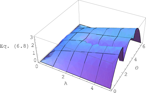
Figure 7: We plot the left-hand side of eq. (72) versus $\theta$ and $A$ for $\eta=2$ GeV.

In general, we cannot give analytical solutions to the equations (72) and (73). However, the fact that, for reasonable values of the parameters, solutions to such equations exist is crucial. In this respect, in figs. 5 and 6 we show that, for $\eta=(0.5,1,2)$ and $A=3$, they can be solved for a constant value and for zero, respectively. In particular, eq. (72) has either zero or six roots depending on the choice of the value for the constant, unlike the case of eq. (73), where at most three zeros can be found depending on the constant.

Following what we say at the beginning of this section, the absolute value of $e^{iw_{f}}$ increases of decreases along the Stokes lines while it remains constant along anti-Stokes lines. Figure 8 displays this behaviour in a neat way.

Figure 8: Here we plot $|e^{iw_{f}}|$ versus $\theta$. The curves have been obtained for $\eta=(1,2)$ (continuous, long dashed) lines (cf eq. (40)) and $A=3$.

VII Concluding remarks and open problems

Second-order equations for relativistic systems have been investigated along many years, including the work in Goldberg , and supersymmetric extensions considered in Cooper . In ordinary quantum mechanics, the most powerful choice of base function is the Langer choice Langer ; Crothers ; Linnaeus , but the peculiar technical difficulties of the effective potentials (2.2) and (2.3) for the Dirac equation cannot be solved in the same way, and one has rather to resort to the JWKB method along the lines in Lazur . It was here our intention to investigate potentialities and limits of the phase-integral method, which actually differs from JWKB methods Froman02 . Our results are of qualitative nature, while we fail to obtain bound-state energies from the integrals in sections 2 and 3. At a deeper level, the problem arises of solving coupled systems of first-order ordinary differential equations which, when decoupled, give rise to a pair of equations of the form (1.1). The phase-integral method, originally developed for second-order equations of the form (1.1), should have implications for the solutions of the original first-order system as well. This expectation should be made precise, and its relation with the JWKB method should be elucidated.

Although the decoupled second-order equations obtained from the radial Dirac equation are formally analogous to the second-order equations to which the phase-integral method can be applied, the actual implementation is much harder because the “potential” terms $R_{f}$ and $R_{g}$ therein contain complicated denominators built from the potentials $V_{S}$ and $V_{V}$ in the radial Dirac equation PHSTB-77-065005 ; JPAGB-32-5643 . This implies that the actual choice of base function $Q$ is a difficult problem. In Sec. III we have described some possible choices of $Q$, and in Sec. IV we have arrived at the majorization (4.9) to select $Q$, tested numerically in Sec. V. The analysis of (4.9) for the Cornell potential shows that an appropriate basis function can be found for the case $k=-1$ (see fig. 3). Moreover, for the logarithmic potential the plots displayed in fig. 2 show that (4.9) is not fulfilled in the whole range of $r$. The investigation of Stokes and anti-Stokes lines in Sec. VI is also, as far as we know, original in our context. It remains to be seen, however, whether such lines can be of direct phenomenological interest.

The work in Ref. PHSTB-77-065005 , despite being devoted to the amplitude-phase method, did not investigate our same technical issues. Thus, no obvious comparison can be made. The years to come will hopefully tell us whether choices of $Q$ satisfying (4.9) exist for which the $F$-matrix in (2.18) can be actually evaluated. In the affirmative case, one would gain conclusive evidence in favour of the superiority of the phase-integral method. In the negative case, one would instead gain a better understanding of the boundaries to our knowledge.

References

• (1) Fröman N and Fröman P O 2002 Physical Problems Solved by the Phase-Integral Method (Cambridge: Cambridge University Press).
• (2) Olsson M G and Veseli S 1995 Phys. Rev. D 51 5079
• (3) Eichten E et al. 1978 Phys. Rev. D 17 3090; 1980 Phys. Rev. D 21 203
• (4) Thylwe K E 2008 Phys. Scripta 77 065005; 2008 J. Phys. A 41 115304
• (5) Popov V S 1971 JETP 32 151
• (6) Zel’dovich Ya B and Popov V S 1972 Sov. Phys. Usp. 14 673
• (7) Lazur V Yu, Reity O K and Rubish V V 2005 Theor. Math. Phys. 143 559
• (8) Fröman N and Fröman P O 1965 JWKB Approximation. Contributions to the Theory (Amsterdam: North–Holland)
• (9) Kaburagi M, Kawaguchi M, Morii T, Kitazoe T and Morishita J 1980 Phys. Lett. B 97 143
• (10) Goldberg I B and Pratt R H 1987 J. Math. Phys. 28 1351
• (11) Cooper F, Khare A and Sukhatme U 1995 Phys. Rep. 251 267
• (12) Langer R E 1937 Phys. Rev. 51 669
• (13) Crothers D S F 2008 Semiclassical Dynamics and Relaxation (Berlin: Springer–Verlag)
• (14) Linnaeus I J and Thylwe K E 2009 Eur. Phys. J. D 53 283
• (15) Esposito G and Santorelli P 1999 J. Phys. A 32 5643