Random walks and magnetic oscillations in compensated metals

Abstract

The field- and temperature-dependent de Haas-van Alphen oscillations spectrum is studied for an ideal two-dimensional compensated metal whose Fermi surface is made of a linear chain of successive orbits with electron and hole character, coupled by magnetic breakdown. We show that the first harmonics amplitude can be accurately evaluated on the basis of the Lifshits-Kosevich (LK) formula by considering a set of random walks on the orbit network, in agreement with the numerical resolution of semi-classical equations. Oppositely, the second harmonics amplitude does not follow the LK behavior and vanishes at a critical value of the field-to-temperature ratio which depends explicitly on the relative value between the hole and electron effective masses.

I Introduction

Due to their rather simple Fermi surface (FS), organic metals provide a powerful playground for the investigation of quantum oscillation physics. In that respect, the most well known example is provided by $\kappa$-(BEDT-TTF)₂Cu(NCS)₂ which can be regarded as the experimental realization of the FS considered by Pippard in the early sixties for his modelPi62 . Such a FS, composed of closed hole orbits and quasi-one dimensional sheets coupled by magnetic breakdown (MB), yields quantum oscillations spectra with numerous frequency combinations that cannot be accounted for by the semiclassical model of Falicov and StachowiakFa66 . This phenomenon which is attributed, for this kind of FS, to either the formation of Landau bands or (and) the oscillation of the chemical potential in magnetic field has raised a great interestAl96 ; Sa97 ; Fo98 ; Gv02 ; Ch02 ; Ki02 ; Fo05 . Nevertheless, the FS of numerous organic metals is composed of compensated electron- and hole-type closed orbitsRo04 , yielding many frequency combinations as well, as far as Shubnikov-de Haas oscillations are concernedPr02 ; Vi03 ; Au05 . In the case of a FS composed of two compensated orbits coupled to each other through MB but isolated from the other orbits outside the first Brillouin zone (FBZ), it has been shown that the oscillations of the chemical potential can be strongly damped Fo08 which could account for the absence of frequency combinations reported in the de Haas-van Alphen (dHvA) spectra of two-dimensional (2D) networks of compensated orbits in fields up to 28 T Au05 . However, the FS considered in Ref. Fo08, which, to our knowledge, has no counterpart among the compounds synthesized up to now, does not provide a network of orbits and, therefore, do not yield Landau bands in magnetic field.

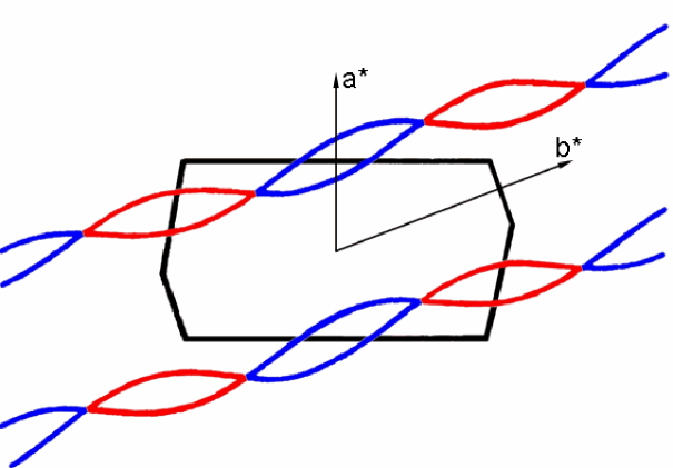
Figure 1: (color online) Calculated Fermi surface of the Bechgaard salt (TMTSF)₂NO₃ in the temperature range below the anion ordering and above the spin density wave condensation, according to Ref. Ka05, . Solid blue and red lines are compensated hole and electron orbits, respectively.

The aim of this paper is to explore the field and temperature dependence of the dHvA oscillations spectra of an ideal 2D metal whose FS achieves a linear chain of successive electron- and hole-type compensated orbits. Such a topology can be relevant in compounds for which the FS originates from an orbit with an area equal to that of the FBZ and coming close to the FBZ boundary along one direction, as it has been predicted for (BEDT-TTF)₄NH₄[Fe(C₂O₄)₃]Pr03 . In this case, a large MB gap is observed at this point and a linear chain of successive electron-hole tubes separated with a smaller MB gap can be observed. Analogous topology is also realized in the Bechgaard salt (TMTSF)₂NO₃ in the temperature range in-between the anion ordering temperature and the spin density wave condensation Ka05 . We will focus on the field- and temperature-dependent amplitude of the first and second harmonics $A_{1}$ and $A_{2}$ of the oscillatory part of the magnetization $M_{osc}$ derived for such FS topology, which can be expanded as $M_{osc}$ = $\sum_{i}A_{i}\sin(2\pi iF_{0}/b)$, where the fundamental frequency of the problem $F_{0}$ and the dimensionless magnetic field $b$ are specified in the next section.

II Model

We consider a 2D metal whose electronic structure consists of two parabolic bands with hole- and electron-character yielding a periodic array of compensated orbits (see Fig. 2). The bottom of the electron band is set at zero energy while the top of the hole band is at $\Delta>0$, with the possibility for the quasiparticle to tunnel through a gap between two successive orbits by MB. The total number of quasiparticles in the system is constant and, to lower the total energy at zero field and zero temperature, the area of the hole-band at the Fermi surface should be equal to the area of the electron-band which accounts for compensation. Indeed, if the hole band were completely filled, the zero-field energy would be higher than if one part of the quasiparticles were transferred from the hole-band to the electron-band. In the following, the effective masses linked to the two bands, $m^{*}_{e}$ and $m^{*}_{h}$, can be different. As in Refs. Fo05, ; Fo08, , the dimensionless field $b$ and temperature $t$ are given by $b=B/\tilde{B}$ and $t=T/\tilde{T}$, respectively, where $\tilde{B}=h/eA_{0}$, $\tilde{T}$= $\tilde{E}/k_{B}$, and $A_{0}$ is the unit cell area. The effective masses and energies are expressed in free electron mass $m_{0}$ units and in units of $\tilde{E}$ = 2$\pi\hbar^{2}m_{0}A_{0}$, respectively. Unit cell area of most organic metals is in the range 100-200 ${\rm\AA^{2}}$ yielding $\tilde{B}$ and $\tilde{T}$ values of few thousands of Tesla and Kelvin, respectively. Therefore, realistic experimental conditions yield small values of $b$ and $t$ compared to $\tilde{B}$ and $\tilde{T}$, respectively. On the contrary, the ratio $b/t$, which is the relevant external parameter for perfect crystals, is given by $b/t=(e\hbar/m_{0}k_{B})$ $B/T$. Its value is close to the $B/T$ ratio achieved in experiments since $e\hbar/m_{0}k_{B}$ $\simeq$ 1.34 KT^-1. Given an energy $E$, the areas of the electron- and hole-type surfaces are respectively $S_{e}=2\pi m_{e}^{*}E$ and $S_{h}=2\pi m_{h}^{*}(\Delta-E)$, which are both quantized for closed orbits in the Brillouin zone. The zero field Fermi energy $\mu_{0}$ is given by the condition of compensation $S_{e}(\mu_{0})=S_{h}(\mu_{0})$ hence $\mu_{0}=[m_{h}^{*}/(m_{e}^{*}+m_{h}^{*})]\Delta$. The fundamental frequency of this system is therefore equal to $F_{0}=S_{e}(\mu_{0})/2\pi=S_{h}(\mu_{0})/2\pi=m_{e}^{*}m_{h}^{*}\Delta/(m_{e}^{*}+m_{h}^{*})$. Each Landau level (LL) has a degeneracy $b$ per sample area. The spectrum of such chain of coupled electron-hole orbits and the quantization of the energy are determined by semi-classical and conservation rules of the wave-function amplitudes at the junctions where the quasiparticles tunnel and across the boundaries of the Brillouin zone. In particular, the amplitude of the wave-function at different points of the Fermi surface (see Fig. 2 for notations) satisfies the following rules: its phase is proportional to the area swept by the quasi-particle around the trajectory divided by $b$. We will note $\sigma_{e}=S_{e}/2b$ and $\sigma_{h}=S_{h}/2b$ the phases around half the electron and hole orbits, respectively. Also, at every junction there is a probability $ip$ for the quasi-particle to tunnel and a probability $q$ to be reflected. Finally we add a Maslov index $i=\sqrt{-1}$ at the vertical extrema of the orbits (cross symbols on Fig. 2). With these rules, we can write the relations between the wave-function amplitudes $\alpha$’s and $\beta$’s:

$$\alpha_{1} = i\exp(i\sigma_{e})(ip\alpha+q\beta),$$

$$\alpha_{2} = ip\alpha_{1}+q\beta_{2},\;\;\alpha^{\prime}=i\exp(-i\sigma_{h})\alpha_{2}$$

$$\beta_{1} = q\alpha_{1}+ip\beta_{2},$$ (1)

$$\beta_{2} = i\exp(-i\sigma_{h})(q\alpha^{\prime}+ip\beta^{\prime}).$$

Figure 2: One dimensional chain of coupled electron and hole orbits. The Brillouin zone is delimited by the dotted lines. Amplitudes are chosen at specific points on the trajectory (see text).

As boundary conditions, we impose that the amplitudes across one Brillouin zone are identical up to an arbitrary phase $\theta$: $\alpha^{\prime}=\alpha\exp(i\theta)$ and $\beta^{\prime}=\beta\exp(i\theta)$. Solving this system of closed equations, we obtain the quantization of the energy which satisfies the spectrum equation

$$\Big{[}1+q^{2}\exp(2i\sigma_{e})-p^{2}\exp i(\sigma_{e}-\sigma_{h}+\theta)\Big{]}\times$$ (2)

$$\Big{[}1+q^{2}\exp(-2i\sigma_{h})-p^{2}\exp i(\sigma_{e}-\sigma_{h}-\theta)\Big{]}$$

$$= -p^{2}q^{2}\Big{[}\exp i(\sigma_{e}-\sigma_{h})+\exp(-2i\sigma_{h}+i\theta)\Big{]}\times$$

$$\Big{[}\exp i(\sigma_{e}-\sigma_{h})+\exp(2i\sigma_{e}-i\theta)\Big{]}$$

We can distinguish two limiting behaviors. For $q=1$ (or, equivalently, $p=0$), the spectrum reduces to $[1+\exp(2i\sigma_{e})]\times[1+\exp(-2i\sigma_{h})]$ = 0 which corresponds to the discrete LL of two independent electron and hole orbits: $S_{e}(E_{n})=2\pi b(n+1/2)$ and $S_{h}(E_{n})=2\pi b(n+1/2)$, with $n$ positive integer. In the opposite case where $q$ = 0, the spectrum corresponds to non-quantized phases $\sigma_{e}(E)-\sigma_{h}(E)=\pm\theta$ since no closed orbit exists in such case (open chain) and therefore magnetic oscillations vanish, leaving the place to a continuum of states. To study numerically the spectrum given by Eq. (2), we first determine the periodicity in energy of the discrete LLs. For that purpose, we assume that $m^{*}_{h}/m^{*}_{e}$=$q_{0}/p_{0}$ where $q_{0}$ and $p_{0}$ are coprime integers that can be as large as needed to approximate the ratio of the two masses. It is indeed useful to express this quantity with a rational number since it allows to consider as necessary only a finite set of solutions of Eq. (2). The minimal periodicity $T_{E}$ of the spectrum is, in this case and for a given phase $\theta$, equal to $T_{E}=2bp_{0}/m_{e}^{*}$, which is twice the periodicity calculated for an isolated system made of one hole and one electron band Fo08 . The number of solutions inside each interval of width $T_{E}$ is found to be equal to $2(p_{0}+q_{0})$ (this number is conserved when $p$ varies and can be counted exactly for $p=0$). Given a set of solutions $E_{eh}(q,n,\theta)$, $n=0,\cdots,2(p_{0}+q_{0})-1$, we introduce a cutoff function $\varphi_{c}(E)$ such as $\varphi_{c}(E)=1$ for $E$ larger than a characteristic energy $E_{c}$ and equal to $\exp[-c(E-E_{c})^{2\delta}]$ for $E\leq E_{c}$, where $\delta$ is any positive integer greater than 1 (we take $\delta=4$ in the simulations which gives a very smooth cutoff function), and $c$ a positive parameter determined self-consistently. This function has the property of preserving the physical features near the Fermi surface and the GS energy is in particular finite since now the corresponding hole spectrum is bounded for large and negative energies. The LL density of states $\rho_{c}(E)$ takes the following form

$$\rho_{c}(E) = \frac{b}{2\pi}\int_{0}^{2\pi}d\theta\sum_{n=0}^{2(p_{0}+q_{0})-1}\sum_{k=-\infty}^{\infty}$$ (3)

$$\varphi_{c}(E)\delta(E-E_{eh}(q,n,\theta)-kT_{E})$$

Given $E_{c}$, the positive parameter $c$ is found to be solution of the equation of conservation at zero temperature:

$$N_{eh} = \int_{-\infty}^{\mu_{0}(b)}dE\rho_{c}(E)$$ (4)

$$= \frac{b}{2\pi}\int_{-\infty}^{\mu_{0}(b)}dE\int_{0}^{2\pi}d\theta\sum_{n=0}^{p_{0}+q_{0}-1}\sum_{k=-\infty}^{\infty}$$

$$\varphi_{c}(E)\delta(E-E_{eh}(q,n,\theta)-kT_{E})$$

where $N_{eh}$ is, as mentioned before, the total number of quasiparticles in the Canonical Ensemble. In the numerical simulations, $\mu_{0}(b)$ is taken as the first LL located below $\mu_{0}$. We choose $N_{eh}$, which is arbitrary, as a multiple of the characteristic zero field energy density $(m_{e}^{*}+m_{h}^{*})\mu_{0}$ (which is proportional to the areas of the Fermi surface). We will also choose in the following $E_{c}=-2$ and $N_{eh}=8(m_{e}^{*}+m_{h}^{*})\mu_{0}$, and 10 values of $\theta$ for the integral evaluations. For each value of the field $b$, the parameter $c$ defined from Eq. (4) is unique and determined self-consistently. Then we can compute for example the GS energy $\Delta E_{0}$

$$\Delta E_{0} = \frac{b}{2\pi}\int_{-\infty}^{\mu_{0}(b)}dE\int_{0}^{2\pi}d\theta\sum_{n=0}^{p_{0}+q_{0}-1}\sum_{k=-\infty}^{\infty}$$

$$E\varphi_{c}(E)\delta(E-E_{eh}(q,n,\theta)-kT_{E})$$ (5)

and the free energy $\Delta F$

$$\Delta F = -\frac{tb}{2\pi}\int_{-\infty}^{\infty}dE\int_{0}^{2\pi}d\theta\sum_{n=0}^{p_{0}+q_{0}-1}\sum_{k=-\infty}^{\infty}\varphi_{c}(E)$$ (6)

$$\log[1+\exp\beta(\mu-E)]\delta(E-E_{eh}(q,n,\theta)-kT_{E})$$

$$+ N_{eh}\mu.$$

The chemical potential $\mu=\mu(t,b)$ is calculated from Eq. (6) by extremizing the free energy $\partial\Delta F/\partial\mu=0$. The magnetization $M_{osc}=-\partial\Delta F/\partial b=x^{2}\partial\Delta F/\partial x$, where $x=1/b$, has to be independent of the parameter $E_{c}$ for $E_{c}$ far away from the chemical potential or at energies large compared to the Landau gap for a given magnetic field. We have checked, for different values of $E_{c}$ with $\Delta=1$, for example $E_{c}=-1,-2,-4$, and for a large range of fields, that the resulting magnetization is stable in this procedure.

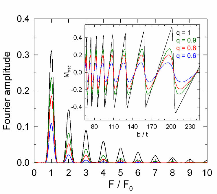
Figure 3: (color online) Fourier spectra of the oscillatory magnetization (displayed in the inset) for various $q$ values. The effective masses are $m_{e}$ = 1 and $m_{h}$ = 2.5. $F_{0}$ is the fundamental frequency (see text).

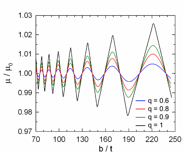
Figure 4: (color online) $b/t$ dependence of the chemical potential normalized to its value $\mu_{0}$ in zero-field for various $q$ values. The effective masses are $m_{e}$ = 1 and $m_{h}$ = 2.5.

Examples of field-dependent dHvA and chemical potential oscillations deduced from the numerical resolution of Eq. 6 are given in Figs. 3 and 4, respectively. These data are derived assuming a constant tunnelling probability $p=\sqrt{1-q^{2}}$ even though $p$ is field-dependent. Nevertheless, a qualitative conclusion can be derived from these data which otherwise will be used in the following for the study of the Fourier amplitudes: the oscillations of the chemical potential are weak, owing to the large $b/t$ range considered, and decrease as $q$ decreases. This point which is in agreement with the conclusion derived for isolated orbitsFo08 confirms that the field-dependent chemical potential oscillations are strongly damped in 2D compensated metals.

III Amplitude of the first harmonics in the LK approximation using random walk analogy

In this section, we compute the expression for the first harmonics amplitude $A_{1}^{LK}$, corresponding to the frequency $F_{0}$, within the LK approximation. We will check numerically that this approximation fits very well the amplitude $A_{1}$ extracted from the spectrum computed in the previous section. We first notice that there are an infinite number of orbits along the chain contributing to this amplitude (see Ref. Fo08, ) since a semi-classical trajectory around a successive electron and hole pockets gives a zero frequency contribution. Therefore these zero frequency orbits can in principle be added to any orbit which has a $F_{0}$ contribution to form new $F_{0}$-orbits by juxtaposition of continuous trajectories. These orbits yielding the frequency $F_{0}$ can be classified by their successive masses $m_{e}(l)=lm_{e}^{*}+(l-1)m_{h}^{*}$ or $m_{h}(l)=(l-1)m_{e}^{*}+lm_{h}^{*}$, where $l$ is a positive integer. The contribution of orbits with large effective mass is negligible at low field or high temperature ($b/t$ small) but have a significant value in the large $b/t$ limit where all the orbits have to be taken into account. Indeed the field- and temperature-dependent damping factors which are defined for a given set of effective masses $m_{e(h)}^{*}$ by the formula

$$R(m_{e(h)}^{*})=\frac{2\pi^{2}m_{e(h)}^{*}t/b}{\sinh(2\pi^{2}m_{e(h)}^{*}t/b)}$$ (7)

are close to unity in this limit. Dingle factors

$$R_{D}(m_{e(h)}^{*},t_{e(h)}^{*})=\exp(-2\pi^{2}m_{e(h)}^{*}t_{e(h)}^{*}/b)$$ (8)

where $t_{e(h)}^{*}=m_{0}A_{0}/4\pi^{2}\hbar\tau_{e(h)}$ are the reduced Dingle temperatures, can also be added to account for real crystals in which the relaxation times $\tau_{e(h)}$ have finite values. In the following we will assume first that these two relaxation times are negligibly small to simplify the calculations. The existence of an infinite set of orbits contributing to the first harmonics leads us to define a closed random walk on the chain in the Brillouin zone $\{x_{i}\}_{i=0,2n}$, with origin and end at $x_{0}$ and $x_{2n}$, respectively, with the condition $x_{0}=x_{2n}=0$. These coordinates take integer values (either negative or positive) and define precisely the pocket inside which the quasiparticle is located. We chose $x_{i}$ with $i$ even to be the positions of the electron bands and $i$ odd for the hole bands. A closed path has an even number of steps $2n$. For a given $x_{i}$, the particle can also orbit a number $n_{i}\geq 0$ of times around the surface before going to the next band. An example of a typical closed trajectory is given in Fig. 5.

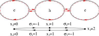
Figure 5: Example of a trajectory contributing to the first amplitude, with fundamental frequency $F_{0}$ and mass $m_{e}(1)=2m_{e}^{*}+m_{h}^{*}$. The successive coordinates $\{x_{i}\}_{i=0,..4}$ of the quasiparticle are given below the figure. Here $n_{i}=0$ (see text). $\sigma_{-1}=-1$ since the particule is going backward when it is reaching the location $x_{0}=x_{4}$ from $x_{-1}=x_{3}$ on a periodic orbit.

We can rewrite coordinates $x_{i}$ by the mean of forward/backward variables $\sigma_{i}=\pm 1$ such as $x_{i}=x_{i-1}+\sigma_{i}(x_{i-1}-x_{i-2})$. Here $\sigma_{i}=1$ when the particle is going forward on its path (in the same direction) and $\sigma_{i}=-1$ when it is going backward in the reverse direction (see Fig. 5 for an explicit set of $\sigma_{i}$’s). The path is moreover made periodic by imposing $x_{i}=x_{i\pm 2n}$ (and the same for variables $\sigma_{i}$). On Fig. 5, $x_{3}=x_{-1}$ and the particle is moving on the reverse direction when it is reaching the point $x_{0}=x_{4}$ along the portion of path $(x_{-1},x_{0},x_{1})$, which implies that $\sigma_{1}=-1$.

It will be also useful in the following to introduce new periodic variables $y_{i}=x_{i}-x_{i-1}=\pm 1$ which satisfy the simple relations $y_{i}=\sigma_{i}y_{i-1}$ and $\sigma_{i}=y_{i}y_{i-1}$. Let us now calculate the total number of possible orbits with a given effective mass $m_{e}(l)$ (or equivalently $m_{h}(l)$ for a hole orbit since the problem is symmetric by exchange of electron and hole masses) and their contribution to the amplitude of the first harmonic $A_{1}^{LK}$ with the fundamental frequency $F_{0}$. If the particle is going forward, there is an amplitude equal to $ip$ to be transmitted from one band to the next one or $ipq$ if the particle is going backward (it has first to perform exactly one reflection with amplitude $q$ on the band edge before being transmitted back through the previous junction). In term of variables $\sigma_{i}$, this is equivalent to write this partial amplitude as $ip[(1+\sigma_{i})+(1-\sigma_{i})q]/2=ip\sqrt{q}e^{K\sigma_{i}}$, with $e^{K}=1/\sqrt{q}$. Then the LK amplitude corresponding to all electron-like contributions can be written as

$$A_{1}^{LK}(e)=\frac{q^{2}R(m_{e}^{*})}{m_{e}^{*}}+\sum_{l\geq 2}\frac{R(m_{e}(l))}{m_{e}(l)}\times$$ (9)

$$\sum_{n=1}^{2(l-1)}\frac{1}{n}\sum_{\{n_{i},\sigma_{i}\}}(-p^{2})^{n}q^{n+2\sum_{j=0}^{2n-1}n_{j}}e^{K\sum_{i=1}^{2n}\sigma_{i}}$$

The sum over $l$ corresponds to all possible masses, and the sum over $n\geq 1$ the number $2n$ of possible tunnellings. The first term $l=1$ in Eq. (9) is the simplest orbit of the expansion: a closed trajectory around one electron pocket with MB damping factor $q^{2}$ and effective mass $m_{e}^{*}$. The sum over $n$ is limited to $2(l-1)$ which corresponds to the extremal trajectory, $i.e$ the particle of mass $m_{e}(l)$ visits a maximum of $(l-1)$ successive electron and hole pockets outside the first initial electron pocket before going back, $l-1$ being also the maximal linear extension of the path. This implies that all the $n_{i}$ are zero for this case (see Fig. 5). The factor $1/n$ takes into account of the orbit symmetry by circular permutation of the coordinates $\{x_{i}\}$. Finally, the sum over the set $\{n_{i},\sigma_{i}\}$ is constrained by the boundary conditions $x_{0}=x_{2n}$ and by the facts that the frequency is set to $F_{0}$ and the effective mass is $lm_{e}^{*}+(l-1)m_{h}^{*}$. This implies the following conditions on $\{n_{i},\sigma_{i}\}$:

$$l = \sum_{j=0}^{n-1}n_{2j}+\frac{n}{2}+\sum_{j=0}^{n-1}\frac{1-\sigma_{2j+1}}{4}$$ (10)

$$l-1 = \sum_{j=0}^{n-1}n_{2j+1}+\frac{n}{2}+\sum_{j=1}^{n}\frac{1-\sigma_{2j}}{4}$$ (11)

The constrained sum can be transformed using two Kronecker integrals around the complex unit circle

$$A_{1}^{LK}(e)=\frac{q^{2}R(m_{e}^{*})}{m_{e}^{*}}+\sum_{l\geq 2}\frac{R(m_{e}(l))}{m_{e}(l)}\times$$ (12)

$$\sum_{n=1}^{2(l-1)}\frac{(-1)^{n}}{n}\sum_{\{n_{i},\sigma_{i}\}}p^{2n}q^{n}e^{K\sum_{j=1}^{2n}\sigma_{j}}\oint\frac{dz}{2i\pi z}\oint\frac{dz^{\prime}}{2i\pi z^{\prime}}\times$$

$$q^{2\sum_{j=0}^{n-1}n_{2j}}z^{-l+\sum_{j=0}^{n-1}n_{2j}+\frac{n}{2}+\sum_{j=0}^{n-1}\frac{1-\sigma_{2j+1}}{4}}\times$$

$$q^{2\sum_{j=0}^{n-1}n_{2j+1}}z^{\prime-l+1+\sum_{j=0}^{n-1}n_{2j+1}+\frac{n}{2}+\sum_{j=1}^{n}\frac{1-\sigma_{2j}}{4}}$$

The sums over the $\{n_{i}=0,\dots,\infty\}$ can be performed exactly, since $q$ is less than unity. We obtain

$$A_{1}^{LK}(e)=\frac{q^{2}R(m_{e}^{*})}{m_{e}^{*}}+\sum_{l\geq 2}\frac{R(m_{e}(l))}{m_{e}(l)}\times$$ (13)

$$\sum_{n=1}^{2(l-1)}\frac{(-1)^{n}}{n}\sum_{\{\sigma_{i}\}}p^{2n}q^{n}e^{K\sum_{i=1}^{2n}\sigma_{i}}\oint\frac{dz}{2i\pi z}\oint\frac{dz^{\prime}}{2i\pi z^{\prime}}\times$$

$$\frac{z^{-l+3n/4}}{(1-q^{2}z)^{n}}\frac{1}{z^{\sum_{j=0}^{n-1}\sigma_{2j+1}/4}}\frac{z^{\prime-l+1+3n/4}}{(1-q^{2}z^{\prime})^{n}}\frac{1}{z^{\prime\sum_{j=1}^{n}\sigma_{2j}/4}}$$

The condition for a closed path is given by $\sum_{j=1}^{2n}y_{j}=0$, with the periodic conditions $y_{0}=y_{2n}$, which imposes in the previous sum the introduction of another Kronecker function. The previous quantities depending on $\sigma_{i}=y_{i}y_{i-1}$ can be rewritten in term of the $y_{i}$’s only. Using the fact that $e^{K}=1/\sqrt{q}$, the sum over the terms involving these variables is given by the quantity

$$Z_{0} = \sum_{\{y_{i}=\pm 1\}}\int_{0}^{2\pi}\frac{d\alpha}{2\pi}e^{i\alpha\sum_{j=1}^{2n}y_{j}}\times$$ (14)

$$\prod_{j=0}^{n-1}(zq^{2})^{-y_{2j}y_{2j+1}/4}(z^{\prime}q^{2})^{-y_{2j+1}y_{2j+2}/4}$$

This is the partition function for a one dimensional periodic Ising model with an imaginary field and alternate complex coupling. Setting the $2\times 2$ transfer matrices $P_{yy^{\prime}}=(zq^{2})^{-yy^{\prime}/4}e^{i\alpha(y+y^{\prime})/2}$ and $P^{\prime}_{yy^{\prime}}=(z^{\prime}q^{2})^{-yy^{\prime}/4}e^{i\alpha(y+y^{\prime})/2}$, $Z_{0}$ can be written as a trace over the product of operators $(PP^{\prime})^{n}$:

$$Z_{0}={\rm Tr}(PP^{\prime})^{n}=\lambda_{+}^{n}+\lambda_{-}^{n}$$ (15)

where $\lambda_{\pm}$ are the eigenvalues of the matrix $PP^{\prime}$. The amplitude can then be written as

$$A_{1}^{LK}(e)=\frac{q^{2}R(m_{e}^{*})}{m_{e}^{*}}+\sum_{l\geq 2}\frac{R(m_{e}(l))}{m_{e}(l)}\times$$ (16)

$$\sum_{n=1}^{2(l-1)}\frac{(-1)^{n}}{n}p^{2n}q^{n}\oint\frac{dz}{2i\pi z}\oint\frac{dz^{\prime}}{2i\pi z^{\prime}}\times$$

$$\frac{z^{-l+3n/4}}{(1-q^{2}z)^{n}}\frac{z^{\prime-l+1+3n/4}}{(1-q^{2}z^{\prime})^{n}}Z_{0}.$$

It is useful to express complex vectors $z=e^{i\theta}$ and $z^{\prime}=e^{i\theta^{\prime}}$ by their angles $\theta$ and $\theta^{\prime}$. Also, setting $\zeta=\sqrt{q}e^{i\theta/4}$, $\zeta^{\prime}=\sqrt{q}e^{i\theta^{\prime}/4}$, $\bar{\zeta}=1/\zeta$ and $\bar{\zeta}^{\prime}=1/\zeta^{\prime}$, we can express the eigenvalues as

$$\lambda_{\pm} = \nu(\theta,\theta^{\prime},\alpha)\pm\sqrt{\nu^{2}+\eta(\theta,\theta^{\prime})},$$ (17)

$$\nu(\theta,\theta^{\prime},\alpha) = \bar{\zeta}\bar{\zeta}^{\prime}\cos(2\alpha)+\zeta\zeta^{\prime},$$

$$\eta(\theta,\theta^{\prime}) = -(\zeta^{2}-\bar{\zeta}^{2})(\zeta^{\prime 2}-\bar{\zeta}^{\prime 2})$$

$$= -(1-q^{2}z)(1-q^{2}z^{\prime})/(q^{2}\sqrt{zz^{\prime}}).$$

Then

$$Z_{0}=2\sum_{i=0}^{n/2}\sum_{j=0}^{i}C_{n}^{2i}C_{i}^{j}\nu^{n-2j}\eta^{j}$$

$$= 2\sum_{i=0}^{n/2}\sum_{j=0}^{i}\sum_{k=0}^{n-2j}C_{n}^{2i}C_{i}^{j}C_{n-2j}^{k}(\zeta\zeta^{\prime})^{n-2j-2k}\eta^{j}\cos^{k}(2\alpha)$$

where we introduced binomial coefficients $C_{n}^{k}=n!/k!(n-k)!$. In the last line, we can perform the integral over $\alpha$ of the integrand $\cos^{k}(2\alpha)$. The resulting integral is not zero only for $k$ even:

$$\int_{0}^{2\pi}\frac{d\alpha}{2\pi}\cos^{2k}(2\alpha)=\frac{1}{2^{2k}}C_{2k}^{k}.$$ (19)

We finally obtain

$$Z_{0}=2\sum_{i=0}^{n/2}\sum_{j=0}^{i}\sum_{k=0}^{n/2-j}C_{n}^{2i}C_{i}^{j}C_{n-2j}^{2k}C_{2k}^{k}\frac{(\zeta\zeta^{\prime})^{n-2j-4k}\eta^{j}}{2^{2k}}.$$

The amplitude $A_{1}^{LK}$ can be rearranged using the previous results like

$$A_{1}^{LK}(e)=\frac{q^{2}R(m_{e}^{*})}{m_{e}^{*}}+\sum_{l\geq 2}\frac{R(m_{e}(l))}{m_{e}(l)}\times$$ (20)

$$\sum_{n=1}^{2(l-1)}2\frac{(-1)^{n}}{n}p^{2n}\sum_{i=0}^{n/2}\sum_{j=0}^{i}\sum_{k=0}^{n/2-j}C_{n}^{2i}C_{i}^{j}C_{n-2j}^{2k}C_{2k}^{k}\frac{(-1)^{j}}{2^{2k}}\times$$

$$\oint\frac{dz}{2i\pi z}\oint\frac{dz^{\prime}}{2i\pi z^{\prime}}\times\frac{z^{-l+n-j-k}}{(1-q^{2}z)^{n-j}}\frac{z^{\prime-l+1+n-j-k}}{(1-q^{2}z^{\prime})^{n-j}}q^{2n-4j-4k}$$

To compute the last two complex integrals, we use the relation for any positive integers $(\alpha,\beta)$

$$\oint\frac{dz}{2i\pi z}\frac{z^{-\alpha}}{(1-q^{2}z)^{\beta}}=C_{\beta+\alpha-1}^{\alpha}q^{2\alpha}$$ (21)

then

$$A_{1}^{LK}(e)=\frac{q^{2}R(m_{e}^{*})}{m_{e}^{*}}+\sum_{l\geq 2}\frac{R(m_{e}(l))}{m_{e}(l)}\times$$

$$\sum_{n=1}^{2(l-1)}(-1)^{n}p^{2n}q^{4l-2n-2}{\cal S}(l,n)$$ (22)

where we defined the following combinatorial quantities

$${\cal S}(l,n)=\frac{2}{n}\sum_{i=0}^{n/2}\sum_{j=0}^{i}\sum_{k=0}^{n/2-j}\frac{(-1)^{j}}{2^{2k}}\times$$

$$C_{n}^{2i}C_{i}^{j}C_{n-2j}^{2k}C_{2k}^{k}C_{l+k-1}^{l-n+j+k}C_{l+k-2}^{l-n+j+k-1}.$$ (23)

These positive integers ${\cal S}(l,n)$ count the number of non-equivalent orbits for a given mass $m_{e(h)}(l)$ and for which the quasiparticle is visiting $2n$ successive pockets. In table I we have reported, for information, the first numbers for increasing values of $l$ from 2 up to 7, using relation (23). For a given $l$, $n$ is taken from 1 to its maximum value $2(l-1)$.

Table 1: First values of coefficients ${\cal S}(l,n)$ representing the number of non-equivalent orbits for a given mass $m_{e(h)}(l)$ with $2n$ magnetic breakdowns, $1\leq n\leq 2(l-1)$.

${}_{n}\backslash^{l}$	2	3	4	5	6	7
1	2	2	2	2	2	2
2	1	9	23	43	69	101
3		8	68	264	720	1600
4		1	63	610	3080	10925
5			18	584	6132	36980
6			1	228	5950	66374
7				32	2800	64952
8				1	600	34550
9					50	9650
10					1	1305
11						72
12						1

Finally, the total amplitude for the first harmonics is given by the sum of hole and electron contributions:

$$A_{1}^{LK}=\frac{F_{0}}{\pi}\Big{[}A_{1}^{LK}(e)+A_{1}^{LK}(h)\Big{]}.$$ (24)

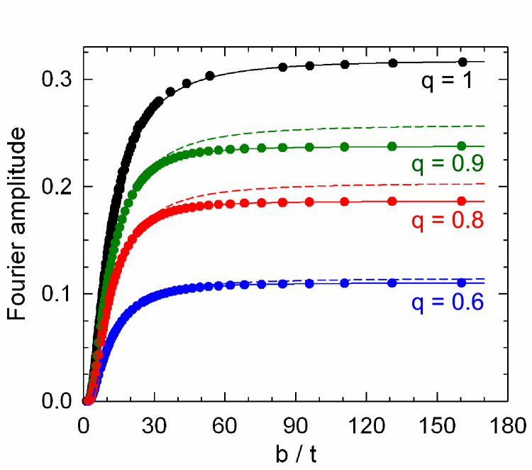
Figure 6: (color online) $b/t$ dependence of the first harmonics amplitude. Solid symbols are deduced from the numerical resolution of Eq. (6). Solid lines correspond to the LK approximation given by Eqs. (22) to (24). Dashed lines correspond to the first order term ($l$=1 in Eqs. (22) ). The effective masses are $m_{e}$=1 and $m_{h}$=2.5.

The first harmonics amplitude is determined by the set of Eqs. (22) to (24). Examples are given in Fig. 6 (solid lines) and compared to the numerical resolution of the Fourier spectrum of the magnetization taken from Eq. (6) (solid symbols) and for different $q$ values. Since the $q$ is fixed, these data can be regarded as temperature-dependent amplitudes at a given field. An excellent agreement between numerical results and Eqs. (22) to (24) is observed, even at high magnetic field. Dashed lines in this figure are the contributions of the first order terms (Eq. 24 reduces to $A_{1}^{LK}=q^{2}F_{0}[R(m_{e}^{*})/m_{e}^{*}+R(m_{h}^{*})/m_{h}^{*}]/\pi$ within this approximation). These terms, which only takes into account the basic orbits with the lowest effective masses ($m_{e}^{*}$ and $m_{h}^{*}$) are strongly dominant since only a small difference (less than 10 $\%$) is observed in the high $b/t$ range. However, as discussed below, the high-order terms with higher effective masses can have a significant influence on the evaluation of the effective masses from experimental data.

In the case of real experimental data collected on q-2D compensated metals, an effective mass $m^{*}$ is deduced from the temperature dependence of the amplitude of the first harmonics $A_{1}$ at a fixed magnetic field. In such a case, it is implicitly assumed that either the effective mass of electron and hole orbits is the same or, oppositely, that only one orbit contributes to the considered Fourier component because the other has a much larger effective mass. In addition, the contribution of high order orbits ($l>$1) is neglected. Taking into account the Dingle damping factor (see Eq. 8), we can rewrite the LK formula as:

$$y\propto R_{MB}\frac{e^{-2\pi^{2}m^{*}t^{*}/b}}{\sinh(2\pi^{2}m^{*}t/b)}$$ (25)

where $y=A_{1}b/t$, $R_{MB}$ is the relevant MB damping factor and $t^{*}$ is the reduced Dingle temperature. If the magnetic field is fixed, Eq. (25) reduces to $y\propto 1/\sinh(2\pi^{2}m^{*}t/b)$. Therefore, the effective mass can be extracted by considering the following combination of derivatives:

$$(2\pi^{2}m^{*})^{2}=2\Big{[}\frac{1}{y}\frac{\partial y}{\partial(t/b)}\Big{]}^{2}-\frac{1}{y}\frac{\partial^{2}y}{\partial^{2}(t/b)}$$ (26)

Figure 7 displays the $b/t$ dependence of $m^{*}$ corresponding to the data in Fig. 6 which stands for a perfect crystal ($t^{*}$=0). For a given $q$ value, the results are scaled as $m^{*}$/min($m^{*}_{e}$, $m^{*}_{h}$). For $q$=1, data analysis based on Eq. (26) yields $m^{*}$/min($m^{*}_{e}$, $m^{*}_{h}$)=1 and $\sqrt{m^{*}_{e}m^{*}_{h}}$/min($m^{*}_{e}$, $m^{*}_{h}$) in the low and high $b/t$ limit, respectively. This point is further supported by considering the mass plot in Fig. 8 which yields a straight line at high $t/b$.

For $q<1$, a strongly non-monotonic $b/t$ dependence of $m^{*}$ is observed in Fig. 7. This behavior is linked to the high order terms ($l>1$ in Eqs. (22), (23)). The $q$-dependence of this behavior is also strongly non-monotonic since numerous zeroes can arise in the coefficients involved in Eq. (22) as $q$ varies. Nevertheless, the effective mass variations are damped for real crystals with finite Dingle temperature, as demonstrated in Fig. 9 for $q$=0.6 where it is assumed that $t^{*}_{e}=t^{*}_{h}$ for simplicity. Assuming a fixed magnetic field of 30 T (which yields a MB field $B_{0}$=30.6 T for $q$=0.6), $t^{*}/b$=0.01 stand for a good crystal with a Dingle temperature $T_{D}$=0.4 K. Oppositely, $t^{*}/b$=1, for which $m^{*}$ is always close to min($m^{*}_{e}$, $m^{*}_{h}$) corresponds to an extremely bad crystal for which $\omega_{c}\tau$ = $b$/$2\pi m^{*}t^{*}$ (where the cyclotron frequency $\omega_{c}=2\pi\hbar b/m_{0}m^{*}A_{0}$ in our units) is much lower than 1 at experimentally accessible fields.

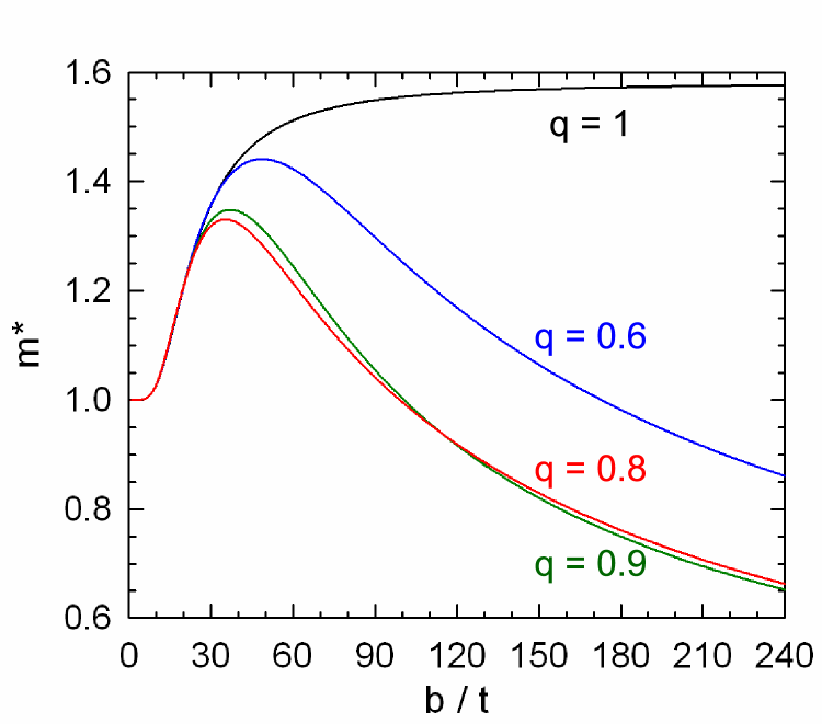
Figure 7: (color online) $b/t$ dependence of the effective mass deduced from Eq. (26) with the parameters relevant to data in Fig. 6.

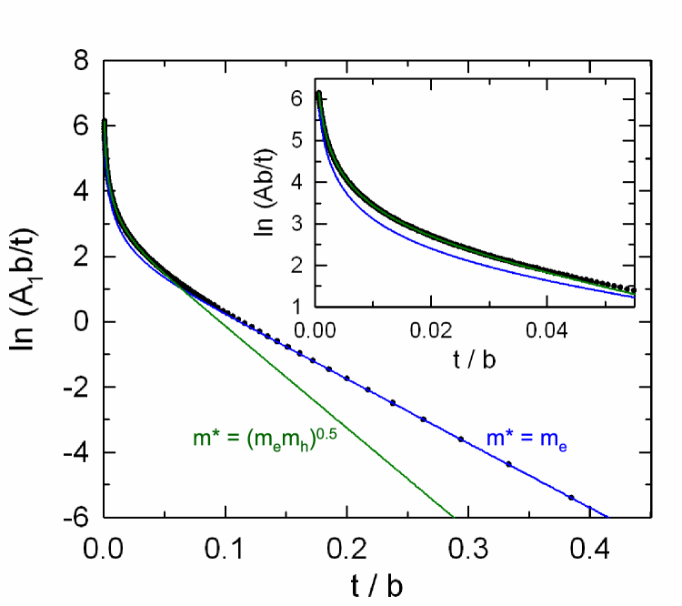
Figure 8: (color online) $t/b$ dependence of $y=A_{1}b/t$ deduced from Eqs. (22) to (24) for $m^{*}_{e}$=1, $m^{*}_{h}$=2.5 and $q$=1 (solid symbols) and best fits of Eq. (26) to this data in the low (blue solid line) and high (green solid line) $t/b$ range. The inset displays the low $t/b$ range.

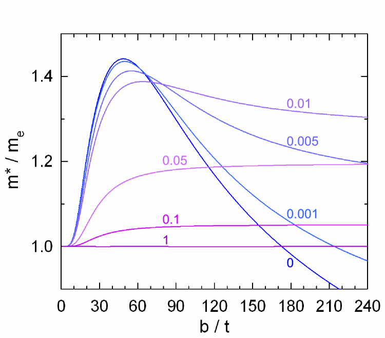
Figure 9: (color online) $b/t$ dependence of the effective mass deduced from Eq. (26) for $m^{*}_{e}$=1, $m^{*}_{h}$=2.5, $q$=0.6 and various values of the Dingle temperature ($t^{*}$) indicated on the curves.

IV Properties of the second harmonics in the Canonical Ensemble

In this section, we study the $t/b$ dependence of the second harmonics. If the analytical expression is difficult to obtain for general parameter $q$, it is however possible to obtain some information in the limiting case $q=1$, which has already been considered in a previous study Fo08 . In particular, we have seen that, in this limit, the free energy $\Delta F$, for a compensated metal, is given by the difference between the Grand potentials of the electron and hole bands, respectively:

$$\Delta F = \Omega_{e}-\Omega_{h}\simeq-m_{e}^{*}\frac{\mu^{2}}{2}-m_{h}^{*}\frac{(\Delta-\mu)^{2}}{2}$$

$$+ \frac{b^{2}}{2m_{e}^{*}}\sum_{n=1}^{\infty}\frac{(-1)^{n}}{\pi^{2}n^{2}}R(nm_{e}^{*})\cos(2\pi nm_{e}^{*}\frac{\mu}{b})$$

$$+ \frac{b^{2}}{2m_{h}^{*}}\sum_{n=1}^{\infty}\frac{(-1)^{n}}{\pi^{2}n^{2}}R(nm_{h}^{*})\cos(2\pi nm_{h}^{*}\frac{\Delta-\mu}{b}).$$

The chemical potential $\mu$ satisfies the self-consistent equation $\partial\Delta F/\partial\mu=0$ given by

$$\mu = \mu_{0}+\frac{b}{m^{*}_{e}+m^{*}_{h}}\sum_{n=1}^{\infty}\frac{(-1)^{n}}{\pi n}[R(nm_{h}^{*})\sin(2\pi nm_{h}^{*}\frac{\Delta-\mu}{b})$$ (28)

$$- R(nm_{e}^{*})\sin(2\pi nm_{e}^{*}\frac{\mu}{b})].$$

We follow the appendix $B$ of reference (Fo08, ) to extract (for small field values) the second harmonics from equations (IV, 28). The oscillatory part of the magnetization is given by $M_{osc}=-\partial\Delta F/\partial b=x^{2}\partial\Delta F/\partial x$ (we remind that $x=1/b$). We then introduce the periodic function

$$G(x)=\sum_{n=1}^{\infty}\frac{(-1)^{n}}{\pi n}[R(nm_{h}^{*})-R(nm_{e}^{*})]\sin(2\pi nF_{0}x)$$ (29)

so that the chemical potential Eq. (28) can be expressed as $\mu=\mu_{0}+bG(x)/(m^{*}_{e}+m^{*}_{h})$, and the magnetization

$$M_{osc} \approx -\frac{1}{(m_{e}^{*}+m_{h}^{*})}G(x)G^{\prime}(x)$$

$$+ \frac{1}{2}\sum_{n=1}^{\infty}\frac{(-1)^{n}}{\pi^{2}n^{2}}\Re\Big{[}$$

$$\frac{R(nm_{e}^{*})}{m_{e}^{*}}\frac{\partial}{\partial x}\exp(2i\pi nF_{0}x+2i\pi nw_{e}G(x))$$

$$+ \frac{R(nm_{h}^{*})}{m_{h}^{*}}\frac{\partial}{\partial x}\exp(2i\pi nF_{0}x-2i\pi nw_{h}G(x)\Big{]}$$

with $w_{e(h)}=m_{e(h)}^{*}/(m_{e}^{*}+m_{h}^{*})$. We make the further approximation in the exponential parts of (IV), and which is valid at low temperature, that $G(x)$ can be truncated to the first term $G(x)\approx[R(m_{e}^{*})-R(m_{h}^{*})]\sin(2\pi F_{0}x)/\pi$ so that

$$e^{2i\pi nw_{e(h)}G(x)}=\sum_{m=-\infty}^{\infty}J_{m}(n\alpha_{e(h)})\exp(2i\pi mF_{0}x)$$ (31)

where $\alpha_{e(h)}=2m_{e(h)}[R(m_{e}^{*})-R(m_{h}^{*})]/(m_{e}^{*}+m_{h}^{*})$, and $J_{m}$ are the Bessel functions of integer order. Putting expression (31) inside (IV), we then select, in order to isolate the second harmonics, integers such that $n+m=\pm 2$ and $n-m=\pm 2$ for the electron and hole contributions, respectively. Expanding the magnetization in terms of Fourier components $M_{osc}=A_{1}\sin(2\pi F_{0})+A_{2}\sin(4\pi F_{0})+\dots$, we find that the coefficient $A_{2}$ satisfies the relation

$$\frac{\pi A_{2}}{2F_{0}}=-\frac{(R(m_{h}^{*})-R(m_{e}^{*}))^{2}}{2(m_{e}^{*}+m_{h}^{*})}+$$

$$\sum_{n\geq 1}\frac{[R((n+2)m_{h}^{*})-R((n+2)m_{e}^{*})][R(nm_{h}^{*})-R(nm_{e}^{*})]}{n(n+2)(m_{e}^{*}+m_{h}^{*})}$$

$$- \sum_{n\geq 1}\frac{1}{n^{2}}\Big{[}\frac{R(nm_{e}^{*})}{m_{e}^{*}}(J_{n-2}(n\alpha_{e})-J_{n+2}(n\alpha_{e}))$$

$$+ \frac{R(nm_{h}^{*})}{m_{h}^{*}}(J_{n-2}(n\alpha_{h})-J_{n+2}(n\alpha_{h}))\Big{]}.$$

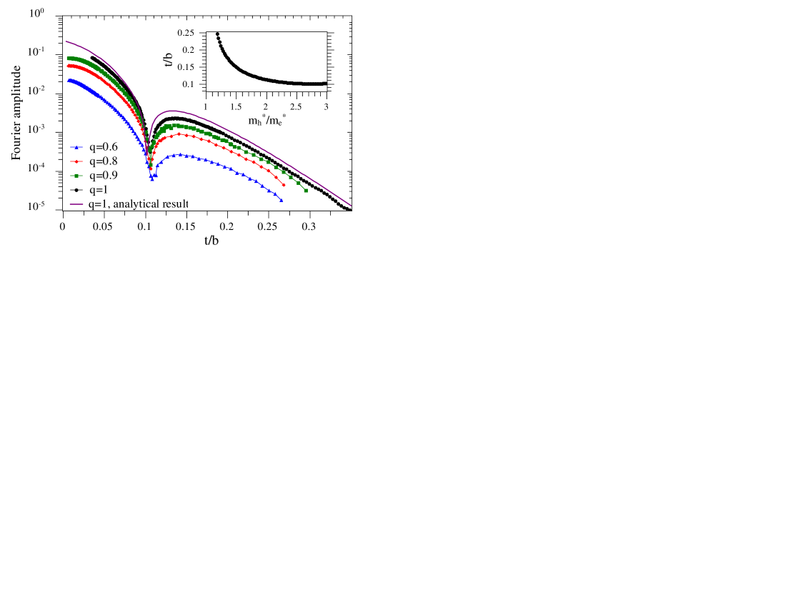
Figure 10: (color online) t/b dependence of the second harmonics amplitude $A_{2}$ for various $q$ values. Solid symbols and solid line correspond to the numerical resolution of Eq. 6 and to the solution of approximation (IV) for $q=1$, respectively. Here $m_{e}^{*}=1$ and $m_{h}^{*}=5/2$. In the insert is plotted the critical value of $t/b$ at which $A_{2}$ vanishes as function of the ratio $m_{h}^{*}/m_{e}^{*}$.

In Fig. 10 is plotted the expression (IV) together with the numerical results obtained by solving directly the spectrum (2) and extracting the second harmonics amplitude for different values of $q$ (see section 2). The two results at $q=1$ agree quite well for a large domain of $t/b$. Remarkably, the numerical data show that, whatever the $q$ value is, the amplitude vanishes at a unique value of $t/b$ depending on the ratio of the two effective masses only. In the example given by $m_{e}^{*}=1$ and $m_{h}^{*}=5/2$, the amplitude vanishes for $t/b\simeq 0.1$. This behavior is strikingly different from that of $A_{1}=A_{1}^{LK}$, considered in previous section, for which no singularity is observed. This reflects the fact that the deviation from the LK approximation appears only in the second harmonic.

V Summary and conclusion

The spectrum for one-dimensional chain of compensated orbits has been calculated. As it is the case for two isolated orbits, the field-dependent oscillations of the chemical potential are weak. In turns, the LK formalism can be applied, provided MB orbits, which in such a network contributes to the fundamental Fourier component amplitude, although with higher effective masses, are taken into account. The resulting high order terms ($l>$ 1 in Eqs. (22) and (23)) can lead to apparent temperature-dependent effective mass for clean crystals in the high $b/t$ limit in the case where only one effective mass is considered for the data analysis, as it is usually done. On the contrary, strong deviation from the LK behavior is observed for the second harmonics. The main feature of this latter component being the zero amplitude occurring at a $t/b$ value depending only on the effective mass ratio $m^{*}_{h}/m^{*}_{e}$. Finally, it can be remarked that the studied 1D-chain does not yield frequency combinations, only harmonics of the fundamental frequency. In a next step, it is planned to consider 2D networks of compensated orbits which account for the FS of many organic metals and are known to give rise to such phenomenon.

References

- [1] A.B. Pippard. Proc. R. Soc. London, A 270:1, 1962.
- [2] L. M. Falicov and Henryk Stachowiak. Phys. Rev., 147(2):505–515, Jul 1966.
- [3] A. S. Alexandrov and A. M. Bratkovsky. Phys. Rev. Lett., 76:1308, 1996.
- [4] P. S. Sandhu, J. H. Kim, and J. S. Brooks. Phys Rev B, 56:11566, 1997.
- [5] Jean-Yves Fortin and Timothy Ziman. Phys. Rev. Lett., 80(14):3117, 1998.
- [6] V. M. Gvozdikov, Y. V. Pershin, E. Steep, A. G. M. Jansen, and P. Wyder. Phys Rev B, 65(16):165102, 2002.
- [7] T. Champel. Phys Rev B, 65:153403, 2002.
- [8] K. Kishigi and Y. Hasegawa. Phys Rev B, 65:205405, 2002.
- [9] J. Y. Fortin, E. Perez, and A. Audouard. Phys Rev B, 71:155101, 2005.
- [10] R. Rousseau, M. Gener, and E. Canadell. Adv. Func. Mater., 14:201, 2004.
- [11] C. Proust, A. Audouard, L. Brossard, S. Pesotskii, R. Lyubovskii, and R. Lyubovskaya. Phys Rev B, 65:155106, 2002.
- [12] D. Vignolles, A. Audouard, L. Brossard, S. Pesotskii, R. Lyubovskii, M. Nardone, E. Haanappel, and R. Lyubovskaya. Eur Phys J B, 31:53, 2003.
- [13] A. Audouard, D. Vignolles, E. Haanappel, I. Sheikin, R. B. Lyubovskii, and R. N. Lyubovskaya. Europhys. Lett., 71:783, 2005.
- [14] J. Y. Fortin and A. Audouard. Phys Rev B, 77:134440, 2008.
- [15] W. Kang, K. Behnia, D. Jérome, L. Balicas, E. Canadell, M. Ribault, and J. M. Fabre. Europhys . Lett., 29:635, 1995.
- [16] T. G. Prokhorova, S. S. Khasanov, L. V. Zorina, L. I. Buravov, V. A. Tkacheva, A. A. Baskakov, R. B. Morgunov, M. Gener, E. Canadell, R. P. Shibaeva, and E. B. Yagubskii. Adv. Funct. Mater., 13:403, 2003.