How effective delays shape oscillatory dynamics in neuronal networks

Abstract

Synaptic, dendritic and single-cell kinetics generate significant time delays that shape the dynamics of large networks of spiking neurons. Previous work has shown that such effective delays can be taken into account with a rate model through the addition of an explicit, fixed delay [1, 2]. Here we extend this work to account for arbitrary symmetric patterns of synaptic connectivity and generic nonlinear transfer functions. Specifically, we conduct a weakly nonlinear analysis of the dynamical states arising via primary instabilities of the asynchronous state. In this way we determine analytically how the nature and stability of these states depend on the choice of transfer function and connectivity. We arrive at two general observations of physiological relevance that could not be explained in previous works. These are: 1 - Fast oscillations are always supercritical for realistic transfer functions. 2 - Traveling waves are preferred over standing waves given plausible patterns of local connectivity. We finally demonstrate that these results show a good agreement with those obtained performing numerical simulations of a network of Hodgkin-Huxley neurons.

1 Introduction

When studying the collective dynamics of cortical neurons computationally, networks of large numbers of spiking neurons have naturally been the benchmark model. Network models incorporate the most fundamental physiological properties of neurons: sub-threshold voltage dynamics, spiking (via spike generation dynamics or a fixed threshold), and discontinuous synaptic interactions. For this reason, networks of spiking neurons are considered to be biologically realistic. However, with few exceptions, e.g. [5, 3, 4], network models of spiking neurons are not amenable to analytical work and thus constitute above all a computational tool. Rather, researchers use reduced or simplified models which describe some measure of the mean activity in a population of cells, oftentimes taken as the firing rate (for reviews, see [6, 7]). Firing-rate models are simple, phenomenological models of neuronal activity, generally in the form of continuous, first-order ordinary differential equations [8, 9]. Such firing-rate models can be analyzed using standard techniques for differential equations, allowing one to understand the qualitative dependence of the dynamics on parameters. Nonetheless, firing-rate models do not represent, in general, proper mathematical reductions of the original network dynamics but rather are heuristic, but see [10]. As such, there is in general no clear relationship between the parameters in the rate model and those in the full network of spiking neurons, although for at least some specific cases quasi-analytical approaches may be of value [11]. It therefore behooves the researcher to study rate models in conjunction with network simulations in order to ensure there is good qualitative agreement between the two.

Luckily, rate models have proven remarkably accurate in capturing the main types of qualitative dynamical states seen in networks of large numbers of asynchronously spiking neurons. For example, it is well known that in such networks the different temporal dynamics of excitatory and inhibitory neurons can lead to oscillations. These oscillations can be well captured using rate models [8]. When the pattern of synaptic connectivity depends on the distance between neurons, these differences in the temporal dynamics can also lead to the emergence of waves [9, 12, 13, 14]. This is certainly a relevant case for local circuits in cortical tissue, where the likelihood of finding a connection between any two neurons decreases as a function of the distance between them, e.g. [15].

When considering the spatial dependence of the patterns of synaptic connectivity between neurons, one must take into account the presence of time delays due to the finite velocity propagation of action potentials along axons. Such delays depend depend linearly on the distance between any two neurons. This has been the topic of much theoretical study using rate models with a space-dependent time delay e.g. [16, 17, 21, 14, 13, 18, 20, 23, 19, 22, 24]. The presence of propagation delays can cause an oscillatory instability of the unpatterned state leading to homogeneous oscillations and waves [17, 20]. The weakly nonlinear dynamics of waves in spatially extended rate models, i.e. describing large-scale (on the order of centimeters) activity, is described by the coupled mean-field Ginzburg-Landau equations [22], and thus exhibits the phenomenology of small amplitude waves familiar from other pattern forming systems [25]. Also, it is important to note that discrete fixed delays have been used to model the time delayed interaction between discrete neuronal regions, as well as to model neuronal feedback, e.g. [26, 29, 27, 28, 30].

Localized solutions of integro-differential equations describing neuronal activity, including fronts and pulses, are also affected by distance-dependent axonal delays [13, 14, 17, 18, 19]. Specifically, the velocity of propagation of the localized solution is proportional to the conduction velocity along the axon for small conduction velocities, while for large conduction velocities it is essentially constant. This reflects the fact that the propagation of activity in neuronal tissue is driven by local integration in which synaptic and membrane time constants provide the bottleneck. Also, allowing for different conduction velocities for separate excitatory and inhibitory populations can lead to bifurcations of localized bump states to breathers and traveling pulses [23].

Although the presence of time delays in the nervous system are most often associated with axonal propagation, significant time delays are also produced by the synaptic kinetics and single-cell dynamics (see the next section for a detailed discussion about the origin of such effective time delays in networks of spiking neurons). As a relevant example for the present work, it was shown in [1, 2] that the addition of an explicit, non-space-dependent delay in a rate equation was sufficient to explain the emergence of fast oscillations prevalent in networks of spiking neurons with strong inhibition and in the absence of any explicit delays.

Specifically, in [1, 2] the authors studied a rate model with a fixed delay on a ring geometry with two simplifying assumptions. First they assumed that the strength of connection between neurons could be expressed as a constant plus the cosine of the distance between the neurons. Secondly, they assumed a linear rectified form for the transfer function which relates inputs to outputs. These assumptions allowed them to construct a detailed phase diagram of dynamical states, to a large degree analytically. In addition to the stationary bump state (SB) which had been studied previously [31, 32], the presence of a delay led to two new states arising from primary instabilities of the stationary uniform state (SU): an oscillatory uniform state (OU) and a traveling wave state (TW). Secondary bifurcations of these three states (SB,OU,TW) led to yet more complex states including standing waves (SW) and oscillatory bump states (OB). Several regions of bistability between primary and secondary states were found, including OU-TW, OU-SB and OU-OB. They subsequently confirmed these results through simulations of networks of Hodgkin-Huxley neurons. Despite the good agreement between the rate equation and network simulations, several important issues remain unresolved:

• The rate equation predicted that the primary instability of the SU state to waves should be to traveling waves, while in the network simulations standing waves were robustly observed.

• The linear-threshold transfer function, albeit amenable to analysis, nonetheless leads to degenerate behavior at a bifurcation point. Specifically, any perturbations with a positive linear growth rate will continue to grow until the lower threshold of the transfer function is reached. This means that the amplitude of new solution branches at a bifurcation is always finite, although the solution itself may not be subcritical. In a practical sense then, this means that it is not possible to assess whether a particular solution, for example oscillations or bumps, will emerge continuously from the SU state as a parameter is changed, or if it will appear at finite amplitude and therefore be bistable with the SU state over some range.

• The previous work only considered a simplified cosine connectivity. More realistic patterns of synaptic connectivity such as a Gaussian dependence of connection strength as a function of distance might lead to different dynamical regimes. It remains to be explored the effect of a general connectivity kernel in the dynamics of both the rate equation and the spiking neurons network with fixed time delays.

In order to address these issues, and provide a more complete analysis of the role of fixed delays in neuronal tissue, we here study a rate equation with delay without imposing any restrictions on the form of the transfer function beyond smoothness or on the shape of the connectivity kernel beyond being symmetric. Our approach is similar to that of Curtu and Ermentrout in [33], who extended a simplified rate model with adaptation for orientation selectivity [32] to include a nonlinear transfer function and general connectivity kernel. Here we do the same for a rate model with a fixed time delay.

Thus in what follows we will study a rate equation with fixed delay and spatially modulated connectivity. In conjunction with this analysis we will conduct numerical simulations of a network of large numbers of spiking neurons in order to assess the qualitative agreement between the rate model and the network for the delay-driven instabilities, which are the primary focus of this work.

This article is organized as follows: In section 2 we provide an overview of the origin of the effective delay. We do this by looking at the dynamics of synaptically coupled conductance-based neurons. This will motivate the presence of an explicit fixed delay in a rate-model description of the dynamics in recurrently coupled networks of neurons. In section 3 we formulate the rate model and conduct a linear stability analysis of the SU state. In section 4 we conduct a weakly nonlinear analysis for the four possible primary instabilities of the SU state (asynchronous unpatterned state in a network model), thereby deriving amplitude equations for a steady, Turing (bumps), Hopf (global oscillations), and Turing-Hopf (waves) bifurcations. We will focus on the delay-driven instabilities, i.e. Hopf and Turing-Hopf. Finally, in section 5 we will study the interactions of pairs of solutions: bumps and global oscillations, and global oscillations and waves, respectively.

2 The origin of effective time delays

This section is intended to provide an intuitive illustration of the origin of an effective fixed delay in networks of spiking neurons. A detailed, analytical study of this phenomenon can be found in [3, 34, 35].

Fig.1 illustrates the origin of the effective delay in networks of model neurons. In this case we look at a single neuron pair: one presynaptic and one postsynaptic. The single-neuron dynamics are described in detail in A. The top panel of Fig.1 shows the membrane potential of an excitatory neuron subjected to a current injection of $I_{app}=0.2\mu$A/cm² which causes it to fire action potentials. Numerically, an action potential is detected whenever the membrane voltage exceeds $0$mV from below. When this occurs, an excitatory postsynaptic current (EPSC) is generated in the post-synaptic neuron, as seen in the second panel. This current is generated by the activation of an excitatory conductance which has the functional form of a difference of exponentials with rise time $\tau_{1}=1$ms and decay time $\tau_{2}=3$ms. The different colored curves correspond to different conductance strengths: black $g_{E}=0.05$, red $g_{E}=0.1$, blue $g_{E}=0.2$ and orange $g_{E}=0.4$ mS$\cdot$ms/cm². The resulting excitatory postsynaptic potential (EPSP) in millivolts is shown in the third panel. At this point it is already clear that the postsynaptic response, although initiated here simultaneously with the presynaptic action potential, will nonetheless take a finite amount of time to bring the postsynaptic cell to threshold, thereby altering its firing rate. This is shown in the bottom panel. In this case the weakest input (black) was insufficient to cause the neuron to spike, while the other three inputs were all strong enough to cause an action potential. The latency until action potential firing is a function of the synaptic strength, with the latency going to zero as the synaptic strength goes to infinity. The very long latency for $g_{E}=0.1$ mS$\cdot$ms/cm² (red curve) is due in part to the intrinsic action potential generating mechanism. In fact, an input which brings the neuron sufficiently close to the bifurcation to spiking can generate arbitrarily long latencies.

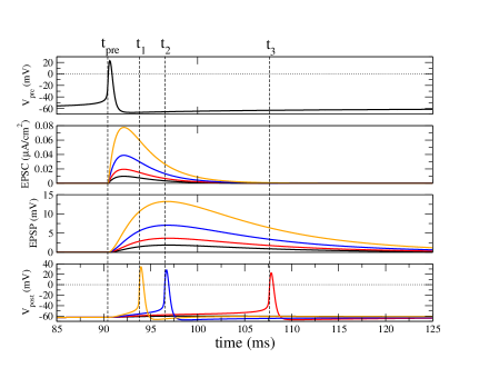
Figure 1: (Color online) The synaptic time course introduces an effective fixed delay in the interaction between model neurons. Top panel: The membrane voltage of the presynaptic neuron which is driven by a steady input current of $I_{app}=0.2\mu$A/cm² causing it to spike periodically. Here only one action potential is shown. The time of the action potential, defined as the time at which the membrane potential crosses zero mV from below, is indicated by the dashed line labeled $t_{pre}$. Second panel from top: The EPSC in the postsynaptic cell is initiated at time $t_{pre}$ with no delay. It consists of a difference-of-exponential conductance change with rise and decay times of $1$ and $3$ milliseconds respectively, times the voltage of the postsynaptic cell (the reversal potential for excitatory synapses is $0$mV). The colors indicate different values of the maximum conductance: black $g_{E}=0.05$, red $g_{E}=0.1$, blue $g_{E}=0.2$ and orange $g_{E}=0.4$ mS$\cdot$ms/cm². See A for details of the model and explanation of units. Third panel from top: The EPSP in the postsynaptic cell. These curves were generated by eliminating the action potential generating currents from the model, i.e. Na and K, and subtracting off the rest potential $\sim-64$mV. Bottom panel: The membrane potential of the postsynaptic cell with $Na$ and $K$ currents intact. Note that the time of the postsynaptic action potential, indicated by the dashed lines, approaches $t_{pre}$ with increasing synaptic strength. The very long latency at time $t_{3}$ is due to an input which puts the cell membrane potential very close to threshold and is therefore due in part to the action potential generating mechanism of the model. The postsynaptic cell is driven by a steady input current of $I_{app}=0.1\mu$ A/cm² which is insufficient to cause it to spike.

Fig.2 illustrates how this effective delay is proportional to both the rise and decay time of the EPSC. In the top panel, the decay time is fixed at $3$ms while the rise time is varied, while in the bottom panel, the rise time is fixed at $0.1$ms and the decay time is varied. From these figures it is clear that the effective delay is proportional to both the rise and decay times. Simulations with an EPSC modeled by a jump followed by a simple exponential decay reveal that the effective delay is proportional to the decay time in this case (not shown).

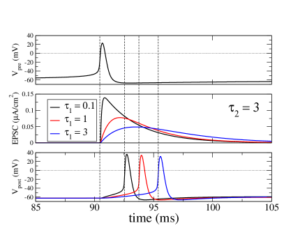
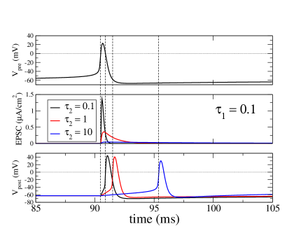
Figure 2: (Color online) The effective delay is affected by both the rise and decay time of the EPSC. Top: The decay is kept fixed at $3ms$ and the rise time is varied. Bottom: The rise time is kept fixed at $0.1$ms and the decay time is varied. The parameter values are the same as in Fig.1 with $g_{E}=0.4$ mS$\cdot$ ms/cm².

It is instructive to note that the effective delay, due to the time course of the synaptic kinetics in the model neuron, can be captured by modeling the EPSC as a Dirac delta function with a fixed delay. This is shown in Fig.3. In Fig.3, the curves shown in black are the same as in Fig. 1 for $g_{E}=0.4$ mS$\cdot$ms/cm², while the red EPSC is a Dirac delta function which arrives with a fixed delay of $3.2$ms. Note that the decay of the EPSP and the postsynaptic spike time are well captured here.

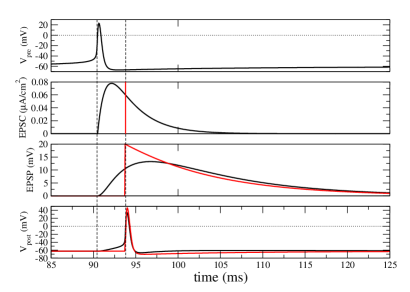
Figure 3: (Color online) Continuous synaptic kinetics can be replaced by a jump in the voltage which occurs at a fixed delay. The black curves in the four panels are the same as in Fig.1 with $g_{E}=0.4$ mS$\cdot$ms/cm². The red curves show the effect of an EPSC modeled as a Dirac delta function which occurs with a delay of $3.2$ms after the presynaptic action potential.

The fact that a jump in voltage with a fixed delay can capture the effect of having continuous synaptic kinetics was described already in [3]. In that work, the authors studied a network of recurrently coupled integrate-and-fire neurons with inhibitory synapses, the time course of which was modeled as jump in the voltage at a fixed delay. They showed that the fixed delay led to the emergence of fast oscillations, the period of which was proportional to approximately several times the delay. The advantage of using EPSCs modeled as Dirac delta functions is that the input current is delta-correlated in time, allowing one to solve the associated Fokker-Planck equation for the distribution of the membrane voltages in a straightforward way.

Subsequent work studied the emergence of fast oscillations in networks of integrate-and-fire neurons with continuous synaptic kinetics [34]. There the authors determined the frequency of oscillations analytically and found that it is proportional to both the rise and decay times of the synaptic response. An extension of that work showed that for networks of Hogkin-Huxley conductance-based neurons, the frequency of oscillations also depends on the single cell dynamics and specifically the membrane time constant and action potential generation mechanism [35]. This is consistent with the effect of the synaptic response and single-cell dynamics on the response latency that we have illustrated above.

Thus the same mechanism which generates an effective delay in the response of a postsynaptic neuron to a single excitatory presynaptic input, can also generate coherent oscillations in a network of neurons coupled through inhibitory synapses. This can be seen in Fig. 4, which shows the results of simulations of a network of $2000$ recurrently coupled inhibitory cells. The single-cell model is the same conductance based model used in Figs.1 -3, see A for details. Synaptic connections are made between neurons with a probability of $p_{0}=0.2$, leading to a sparse, random connectivity with each cell receiving an average of $400$ connections. Synapses are modeled as the difference of exponentials with a rise time and a decay time of $1$ms and $3$ms respectively and $g_{I}=0.01$ mS$\cdot$ms/cm². All cells receive uncorrelated Poisson inputs with a rate of $12000$Hz and $g_{ext}=0.0019$mS$\cdot$ms/cm², and there is no delay in the interactions. Fig. 4A shows a raster plot of the network activity in the top panel. The activity is noisy although periods of network synchrony are visible. The middle panel shows the firing rate averaged over all neurons in time bins of $0.1$ms (black) and smoothed by averaging with a sliding window of $10$ms (red). The large fluctuations in the firing rate indicate network synchrony, while the averaged trace shows clear periodic oscillations. This is even more evident in the bottom panel which shows the subthreshold input current averaged over all cells. One can clearly see the ongoing oscillation, the amplitude of which undergoes slow fluctuations due to the noisy dynamics. Fig. 4B shows the smoothed firing rate (top) and average input current (bottom) from the same simulation, but on a shorter time scale. Note that the sign of the input current has been inverted so that downward deflections mean increasing positive currents. Here it is clear that the input current is a delayed copy of the firing rate, with a delay on the order of $\sim 2-3$ms which matches with the time scale of the synaptic kinetics ($\tau_{1}=1$ms, $\tau_{2}=3$ms).

Therefore, Fig. 4 provides a clear prescription for developing a rate model description of fast oscillations in networks in the asynchronous regime. The input a neuron receives is not simply a nonlinear function of the instantaneous firing rate, rather it is a function of the delayed firing rate. Thus one should introduce a fixed delay in the rate model description. This was the underlying assumption behind the work in [1].

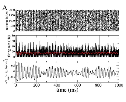
Figure 4: (Color Online) The effective delay can lead to oscillations in networks of recurrently coupled inhibitory neurons. A. Raster plot of the spiking activity in a network of 2000 inhibitory cells (top). The average firing rate shows large fluctuations (center, black), which when smoothed are clearly identifiable as noisy, periodic oscillations (red). Network oscillations are also clearly visible in the average subthreshold input (bottom). B. A blowup of the average firing rate (top) and average input current (bottom) from the simulation in A. The input current is clearly a time-delayed copy of the firing rate. The delay is between $2$ and $3$ms.

Before presenting the model we would like to emphasize that fixed delays, which are primarily due to synaptic and dendritic integration, and conduction delays due to the propagation of action potentials along the axon, are both present in real neuronal systems. Importantly, this means that the delay in neuronal interactions at zero distance is not zero. In fact, fixed delays are always observed in paired intracellular recordings in cortical slices. The latency from the start of the fast rising phase of the action potential to the start of the post-synaptic current (or potential) has been measured for pairs of pyramidal cells in rat layers 3 to 6 and is on the order of milliseconds, see [37] for a recent review. Recordings from cat cortex and between pyramidal cells and other cells including spiny cells and interneurons in the rat cortex also reveal fixed delays which are rarely less than a millisecond. These delays are seen when neurons are spatially adjacent, indicating that axonal propagation is not an important contributing factor. On the other hand the speed of propagation of action potentials along unmyelinated axons in mammals is on the order of $10^{-1}-10^{1}$ m/s, which means a delay of 0.1-10 ms for neurons separated by 1 millimeter [38, 39]. Thus fixed delays and conduction delays are of similar magnitude within a local patch of cortex and both would be expected to shape the dynamics of non-steady activity, i.e. neither is negligible. Here we have decided to focus on fixed delays, as in previous work [1, 2], due both to their physiological relevance and prevalence in networks of spiking neurons.

3 The rate model with fixed time delay

An effective delay roughly proportional to the time scale of the post-synaptic currents is always present in networks of spiking neurons as we have illustrated in the previous section and has been shown extensively elsewhere, e.g. [34, 35]. In particular, this is true for networks in the asynchronous regime, for which a rate-equation description is, in general, appropriate. Given this, we consider here a rate model with fixed delay. Specifically, we study a heuristic equation describing the activity of a small patch of neural tissue consisting of two populations of recurrently coupled excitatory and inhibitory neurons respectively. Our formulation is equivalent to the Wilson-Cowan equations without refractory period [8], and with spatially dependent synaptic connectivity which was studied originally in [40]. Additionally, we consider a fixed delay in the neuronal interactions. Given these assumptions, the full Wilson-Cowan equations are

$$\tau_{e}\dot{r}_{e}=-r_{e}+\Phi_{e}\bigg{[}\int_{\Omega}dy[J_{ee}(|x-y|)r_{e}(y,t-d_{e})-J_{ei}(|x-y|)r_{i}(y,t-d_{i})]+I_{e}\bigg{]},\\$$ (1a)

$$\tau_{i}\dot{r}_{i}=-r_{i}+\Phi_{i}\bigg{[}\int_{\Omega}dy[J_{ie}(|x-y|)r_{e}(y,t-d_{e})-J_{ii}(|x-y|)r_{i}(y,t-d_{i})]+I_{i}\bigg{]}.$$ (1b)

In the original formulation [8], $r_{e}(x,t)$ and $r_{i}(x,t)$ represent the average number of active cells in the excitatory and inhibitory populations respectively, in this case at a position $x$ and at a time $t$. The time constant $\tau_{e}$ ($\tau_{i}$) is roughly the time it takes for a an excitatory (inhibitory) cell receiving “at least threshold excitation” [8] to generate a spike. This can reasonably be taken as the membrane time constant which is generally on the order of 10-20 ms. The functions $\Phi_{a}(x)(a=e,i)$ are usually taken to be sigmoidal. Specifically, if all neurons in the population receive equal excitatory drive, and there is heterogeneity in some parameter across neurons, e.g. the threshold to spiking, which obeys a unimodal distribution, then the fraction of active neurons is just the integral over the distribution, up to the given level of excitation. The integral of a unimodal distribution is sigmoidal. In Eqs.(1a-1b), the functions $J_{ab}(|x|)(a=e,i)(b=e,i)$ represent the strength of synaptic connection from a neuron in population $b$ to a neuron in population $a$ separated by a distance $x$. Here the neurons are arranged in one dimension on a domain $\Omega$. Input from excitatory (inhibitory) cells is furthermore delayed by a fixed amount $d_{e}$ ($d_{i}$), which, as we have discussed in the introduction, is on the order of one millisecond. Finally, the excitatory and inhibitory populations are subject to an external drive of strength $I_{e}$ and $I_{i}$ respectively.

A general analysis of Eqs.(1a-1b) would be technically arduous although it is a natural extension of the work presented here. Rather, we choose to study the dynamics of this system under the simplifying assumption that the excitatory and inhibitory neurons follow the same dynamics, i.e. $\tau_{e}=\tau_{i}=\tau$, $d_{e}=d_{i}=d$, $J_{ee}=J_{ie}=J_{e}$, $J_{ei}=J_{ii}=J_{i}$, $\Phi_{e}=\Phi_{i}=\Phi$, $I_{e}=I_{i}=I$. If this the case, then $r_{e}=r_{i}=r$ and the variable $r$ follows the dynamics given by

$$\dot{r}(x,t)=-r(x,t)+\Phi\bigg{[}\frac{1}{2\pi}\int_{-\pi}^{\pi}dyJ(|x-y|)r(y,t-D)+I\bigg{]},$$ (2)

where we have chosen the domain $\Omega$ to be a ring of normalized length $L=2\pi$. Furthermore, we have re-scaled time by the time constant $\tau$. The normalized delay is therefore $D=d/\tau$, which is the ratio of the effective delay in neuronal interactions to the integration time constant and should be much less than one in general. The synaptic connectivity expressed in terms of the excitatory and inhibitory contributions is $J(|x|)=J_{e}(|x|)-J_{i}(|x|)$, and thus represents an effective mixed coupling which may have both positive and negative regions.

Eq.(2) with the choice of $\Phi(I)=I$ for $x>0$ and 0 otherwise and with $J(x)=J_{0}+J_{1}\cos{(x)}$ is precisely the model studied in [1, 2]. We now wish to study Eq.(2) for arbitrary choices of $\Phi(I)$ and $J(x)$.

In presenting Eq.(2) we have relied on the heuristic physiological motivation first put forth in [8]. Nonetheless, as a phenomenological model, the terms and parameters in Eq.(2) may have alternative and equally plausible interpretations. Indeed, the variable $r$ is often thought of as the firing rate as opposed to the fraction of active cells, in which case the function $\Phi(I)$ can be thought of as the transfer function or fI curve of a cell.

Experimentally the function $\Phi(I)$ has been found to be well approximated by a power-law nonlinearity with a power greater than one [41, 36]. Modeling studies show that the same nonlinearity applies to integrate-and-fire neurons and conductance based neurons driven by noisy inputs [36]. Therefore it may be that such a choice of $\Phi$ leads to better agreement of Eq.(2) with networks of spiking neurons and hence with actual neuronal activity. More fundamentally, we may ask if choosing $\Phi$ as a sigmoid or a power law qualitatively alters the dynamical states arising in Eq.(2). This is precisely why we choose here not to impose restrictions on $\Phi$ but rather conduct an analysis valid for any $\Phi$. How the choice of $\Phi$ affects the generation of oscillations and waves is an issue we will return to in the corresponding sections of this paper.

3.1 Linear stability analysis

Stationary uniform solutions (SU) of Eq.(2) are given by

$$R=\Phi\Big{[}J_{0}R+I\Big{]},$$ (3)

where $R$ is a constant non-zero rate, $J_{0}$ is the zeroth order spatial Fourier coefficient of the symmetric connectivity which can be expressed as

$$J(x)=J_{0}+\left(\sum_{k=1}^{\infty}J_{k}e^{ikx}+c.c.\right)$$ (4)

and $k$ is an integer. Depending on the form of $\Phi$, Eq.(3) may admit one or several solutions.

We study the linear stability of the SU state with the ansatz

$$r(x,t)=R+\sum_{k=0}^{\infty}\delta r_{k}e^{ikx+\alpha(k)t},$$ (5)

where $\delta r_{k}\ll 1$ and the spatial wavenumber $k$ is an integer due to the periodic boundary conditions. Plugging Eq.(5) into Eq.(2) leads to an equation for the complex eigenvalue $\alpha(k)$

$$\alpha(k)=-1+\Phi^{{}^{\prime}}J_{k}e^{-\alpha(k)D},$$ (6)

where the slope $\Phi^{{}^{\prime}}$ is evaluated at the fixed point given by Eq.(3). The real and imaginary parts of the eigenvalue $\alpha(k)=\lambda(k)+i\omega(k)$ represent the linear growth rate and frequency of perturbations with spatial wavenumber $k$ respectively. At the bifurcation of a single mode, the growth rate will reach zero at exactly one point and be negative elsewhere. That is, $\lambda(k_{cr})=0$ for the critical mode $k_{cr}$. Given this, Eq.(6) yields the dispersion relation for the frequency of oscillation of the critical mode

$$i\omega(k_{cr})=-1+\Phi^{{}^{\prime}}J_{k_{cr}}e^{-i\omega(k_{cr})D}.$$ (7)

From Eq.(7) it is clear that the wavelength of the critical mode depends crucially on the synaptic connectivity. In particular, the spatial Fourier coefficients of the connectivity kernel $J(x)$ depend on the wavenumber $k$, i.e. $J_{k}=J(k)$. Thus, the critical wavenumber is, in effect, selected by the choice of connectivity kernel. It is in this way that the nature of the instability depends on the synaptic connectivity at the linear level.

Depending on the values of $\omega$ and $k_{cr}$ in Eq.(7) at the bifurcation from the SU state, four types of instabilities are possible:

• Steady ($\omega=0$, $k_{cr}=0$): The instability leads to a global increase in activity.

• Turing ($\omega=0$, $k_{cr}\neq 0$): The instability leads to a stationary bump state (SU).

• Hopf ($\omega\neq 0$, $k_{cr}=0$): The instability leads to an oscillatory uniform state (OU).

• Turing-Hopf ($\omega\neq 0$,$k_{cr}\neq 0$): The instability leads to waves (SW, TW).

For the non-oscillatory instabilities (i.e. $\omega=0$), Eq.(7) gives the critical value

$$\bar{J}_{k}=1/\Phi^{\prime}$$ (8)

while for the oscillatory ones Eq.(7) is equivalent to the system of two transcendental equations

$$\bar{\omega}=-\tan{\bar{\omega}D},$$ (9a)

$$\bar{\omega}=-\Phi^{{}^{\prime}}\bar{J}_{k}\sin{\bar{\omega}D}.$$ (9b)

Note that we have defined the critical values as $J_{k_{cr}}\equiv\bar{J}_{k}$ and $\omega_{cr}\equiv\bar{\omega}$.

3.1.1 The small delay limit ($D\to 0$)

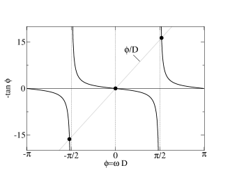
Figure 5: The critical frequency at the instability to oscillations is given by the intersection of the grey ($D=0.1$) and black curves, the left and right hand sides of Eq.(9a) respectively. As $D\to 0$, solutions clearly approach $\phi=(2n+1)\pi/2$ ($n$ integer). Eq.(9b) shows that the first potentially unstable mode corresponds to the solutions $\phi=\pm\pi/2$ (see text).

It is possible to gain some intuition regarding the effect of fixed delays on the dynamics, by deriving asymptotic results in the limit of small delay. This limit is a relevant one physiologically, since fixed delays are on the order of a few milliseconds and the integration time constant is about an order of magnitude larger. Therefore throughout this work we will present asymptotic results, and compare them to the full analytical formulas as well as to numerical simulations.

In the limit $D\to 0$, the asymptotic solutions of Eq.(9a) can be easily obtained graphically. Fig.5 shows two curves (black and grey) representing the right and left hand sides of Eq.(9a) respectively, where we defined $\phi\equiv\bar{\omega}D$. The intersections of these curves correspond to the roots of Eq.(9a). The plot shows three solutions, the trivial one $\phi=0$ (corresponding to the non-oscillatory instabilities), and an infinite number of solutions that clearly approach $\phi=(2n+1)\pi/2$ ($n$ integer) in the small delay limit, since the slope of the straight line goes to infinity as $D\to 0$. Substituting these solutions into Eq. (9b), we find that the first potentially unstable solution of the $k^{th}$ spatial Fourier mode is $\phi=\pm\pi/2$, that occurs at the critical value of the coupling

$$\bar{J}_{k}=-\frac{\pi}{2D\Phi^{{}^{\prime}}},$$ (10)

with a frequency

$$\bar{\omega}=\frac{\pi}{2D}.$$ (11)

Fig. (6) shows the critical frequency and coupling as a function of the delay, up to a delay $D=1$. The solution obtained from the dispersion relation Eqs.(9a) and (9b) are given by solid lines, while the expressions obtained in the small delay limit are given by dotted lines. Thus the expressions in the small delay limit agree quite well with the full expressions even for $D=1$.

Figure 6: Top: The critical frequency of oscillatory instabilities as a function of the delay $D$ from the dispersion equation Eq.(9a) (solid line) and in the small delay limit (dotted line). Bottom: The critical coupling as a function of the delay $D$ from Eq.(9b) (solid) and in the small delay limit (dotted).

3.2 An illustrative Phase Diagram

Throughout the analysis which follows we will illustrate our results with a phase diagram of dynamical states. Specifically, we will follow the analysis in [1, 2] in constructing a phase diagram of dynamical states as a function of $J_{0}$ and $J_{1}$, the first two Fourier coefficients of the synaptic connectivity. We will set the higher order coefficients to zero for this particular phase diagram, although we will discuss the effect of additional modes in the text. Furthermore, unless otherwise noted, for simulations we choose a sigmoidal transfer function $\Phi(I)=\frac{\alpha}{1+e^{-\beta I}}$ with $\alpha=1.5$ and $\beta=3$. As we vary the connectivity in the phase diagram, we also vary the constant input $I$ in order to maintain the same level of mean activity, i.e. we keep $R=0.1$ fixed. For the values of the parameters we have chosen here this results in $I\sim-0.1J_{0}-0.88$. We also take $D=0.1$ unless noted otherwise

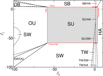
Figure 7: (Color online) Phase diagram of the rate model Eq.(2). In each region, the type of solution seen in numerical simulations is indicated by a letter code: SU - stationary uniform (grey region), HA - high activity, SB - stationary bump, OB - oscillatory bump, SW - standing waves, TW - traveling waves. Solid lines indicate analytical expressions. In particular, the four possible instabilities of the SU state are depicted in red (thick lines correspond to subcritical bifurcations) and are given by the linear stability criteria Eqs.(8-9b). The four lines emanating from the upper and lower left corners of the SU region were determined from a weakly nonlinear analysis at the two corners (codimension two points) [see section IV]. The region marked OB corresponds to a mixed mode solution of SB-OU, while in the lower left-hand region the OU and SW solutions are bistable. Parameters: $\Phi(x)=\frac{\alpha}{1+e^{-\beta x}}$ where $\alpha=1.5$ and $\beta=3$. We consider the coupling function $J(x)=J_{0}+2J_{1}\cos{x}$. The time delay is $D=0.1$ and the input current $I$ is varied so as to keep the uniform stationary solution fixed at $R=0.1$.

The primary instability lines for the SU state can be seen in the phase diagram, Fig. (7). The region in $(J_{0},J_{1})$ space where the SU state is stable is shown in gray, while the primary instabilities, listed above, are shown as red lines. In Section 4 we will provide a detailed analysis of the bumps, global oscillations and waves (SB, OU and SW/TW) which arise due to the Turing, Hopf and Turing-Hopf instabilities respectively. The derivation of the amplitude equations is given in B, as well as a brief discussion of the steady, transcritical bifurcation which occurs for strong excitatory coupling and is not of primary interest for this study. Finally, in Section 5 we will analyze the codimension 2 bifurcations: Hopf and Turing-Hopf (OU and waves), and Turing and Hopf (SU and OU). This analysis will allow us to understand the dynamical states which appear near the upper and lower left hand corners of the grey shaded region in Fig. (7), i.e. the SW/OU and OB states.

4 Bifurcations of codimension 1

As we are interested in creating a phase diagram as a function of the connectivity, we will take changes in the connectivity as the bifurcation parameter. The small parameter $\epsilon$ is therefore defined by the expansion

$$J_{k}=\bar{J}_{k}+\epsilon^{2}\Delta J_{k},$$ (12)

The perturbative method we apply, which makes use of this small parameter, is called the multiple-scales method and is a standard approach for determining the weakly nonlinear behavior of pattern-forming instabilities [25]. We choose the particular scaling of $\epsilon^{2}$ in the foreknowledge that if the amplitudes of the patterns of interest are scaled as $\epsilon$, a solvability condition will arise at order $\epsilon^{3}$. This solvability condition yields a dynamical equation governing the temporal evolution of the pattern (see Appendix A for details). Without loss of generality we will assume that an instability of a nonzero spatial wavenumber is for $k=1$. We will furthermore co-expand the constant input $I$ so as to maintain a fixed value for the spatially homogeneous steady state solution $R$

$$I = \bar{I}+\epsilon^{2}\Delta I,$$ (13)

$$r = R+\epsilon r_{1}+\epsilon^{2}r_{2}+\dots,$$ (14)

where the small parameter $\epsilon$ is defined by Eq.(12). Additionally we define the slow time

$$T=\epsilon^{2}t.$$ (15)

4.1 Turing Bifurcation

The emergence and nature of stationary bumps in rate equations have been extensively studied elsewhere, e.g. [40]. We briefly describe this state here for completeness. The $k^{th}$ spatial Fourier mode of the connectivity is given by the critical value Eq. (8), while we assume that all other Fourier modes are sufficiently below their critical values to avoid additional instabilities. Without loss of generality we assume $k=1$ here.

We expand the parameters $J_{1}$, $I$ and $r$ as in Eqs. (12,13,14), and define the slow time Eq. (15). The solution of Eq.(2) linearized about the SU state $R$ is a spatially periodic amplitude which we allow to vary slowly in time, i.e. $r_{1}=A(T)e^{ix}+c.c.$. Carrying out a weakly nonlinear analysis to third order in $\epsilon$ leads to the amplitude equation

$$\partial_{T}A=\eta\Delta J_{1}A+\Gamma|A|^{2}A,$$ (16)

with the coefficients

$$\eta=\frac{\Phi^{{}^{\prime}}}{1+D},$$ (17a)

$$\Gamma=\frac{\bar{J}_{1}^{3}}{1+D}\Bigg{(}\frac{J_{0}(\Phi^{{}^{\prime\prime}})^{2}}{1-J_{0}\Phi^{{}^{\prime}}}+\frac{J_{2}(\Phi{{}^{\prime\prime}})^{2}}{2(1-J_{2}\Phi^{{}^{\prime}})}+\frac{\Phi^{{}^{\prime\prime\prime}}}{2}\Bigg{)}.$$ (17b)

The nature of the bifurcation (sub- or supercritical) clearly depends strongly on the sign and magnitude of mean connectivity $J_{0}$ and the second spatial Fourier mode $J_{2}$. Figure 8 shows a phase diagram of the bump state at the critical value of $\bar{J}_{1}=3.54$. The red lines indicate oscillatory and steady instability boundaries for the modes $J_{0}$ and $J_{2}$. Clearly $J_{0}<0$ and $J_{2}<0$ over most of the region of allowable values, and the bump is therefore supercritical. There is only a narrow region of predominantly positive values (shaded region in Fig. 8 for which the cubic coefficient is positive. This indicates that the bifurcating solution branch is unstable. However, neuronal activity is bounded, which is captured in Eq.(2) by a saturating transfer function $\Phi$. Thus the instability will not grow without bound but rather will saturate, producing a finite amplitude bump solution. This stable, large amplitude branch and the unstable branch annihilate in a saddle-node bifurcation for values of $J_{1}$ below the critical value for the Turing instability. Such finite-amplitude bumps are therefore bistable with the SU state. In Fig. 8, the two insets show the connectivity kernel $J(x)$ for parameter values given by the placement of the open triangle (subcritical bump) and the open square (supercritical bump).

In the phase diagram (7), the Turing instability line (upper horizontal red line) is shown thin for supercritical, and thick for subcritical bumps (here $J_{2}=0$).

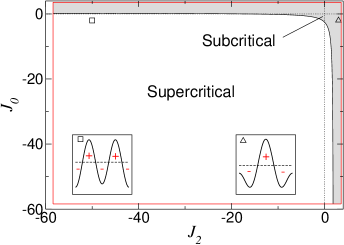
Figure 8: (Color online) The phase diagram for stationary bumps as a function of the zeroth and second spatial Fourier modes of the connectivity kernel. The region of bistability between the unpatterned and the bump state is shaded. Here the critical spatial Fourier coefficient $\bar{J}_{1}=3.54$. Red lines indicate the boundaries of the SU state (obtained via Eqs.(8-9b). The functions $\Phi$ and $J(x)$ as well as the input current $I$ and the delay $D$ are taken as in Fig. (7). Insets: example connectivity patterns corresponding to the values of $J_{0}$ and $J_{2}$ marked by the square and triangle respectively. Note that standard Mexican Hat connectivity tends to favor bistability.

4.2 Hopf Bifurcation

4.2.1 Network simulations

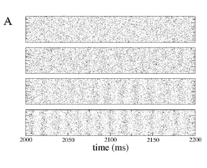
Figure 9: Fast oscillations in a sparse, randomly connected network of 2000 randomly connected inhibitory neurons without delay ($p_{0}^{I}=0.2$). A: Raster plots of spiking activity in four networks with increasing values of the synaptic weight. From top to bottom: $g_{I}=0$, $0.005$, $0.008$, $0.01$mS$\cdot$ms/cm². The mean firing rate was kept fixed at approximately $14$Hz by varying the input current. From top to bottom: $\nu_{ext}=2150$, $7700$, $10000$ and $12000$Hz. See A for additional model details. B: The autocorrelation function of the network-averaged firing rate for the four networks.

As shown elsewhere previously [3, 4, 1], a network of recurrently coupled inhibitory neurons can generate fast oscillations due to the effective delay in the synaptic interactions. Fig.9A shows raster plots of the spiking activity in a network randomly connected inhibitory neurons as the synaptic weight $g_{I}$ is increased (see A for a description of the network). The raster plots clearly show oscillations emerging as the parameter $g_{I}$ increases in strength. Fig.9B shows the autocorrelation function of the network-averaged firing rate from four seconds of simulation time. The curve is completely flat for the uncoupled case as expected, while periodic peaks appear and grow as the synaptic weights are increased, indicating the presence of coherent network oscillations. Note that the oscillations appear to emerge continuously, which would indicate a supercritical bifurcation. This is consistent with the finding in [3], where fast oscillations in a network of integrate-and-fire neurons were shown to be supercritical analytically.

We may ask if fast oscillations are in general expected to bifurcate supercritically, or if a subcritical bifurcation is also possible. To this end we study the rate equation which allows us to detemine the nature of the bifurcation analytically as a function of the transfer function and connectivity.

4.2.2 Rate model

In the rate model there is a spatially homogeneous oscillatory instability with frequency $\omega$ given by Eq.(9a). This occurs for a value of the $0^{th}$ spatial Fourier mode of the connectivity given by Eq.(9b), while we assume that all other Fourier modes are sufficiently below their critical values to avoid additional instabilities. We expand the parameters $J_{0}$, $I$ and $r$ as in Eqs. (12,13,14), and define the slow time Eq. (15). The linear solution has an amplitude which we allow to vary slowly in time, i.e. $r_{1}=H(T)e^{i\omega t}+c.c.$. Carrying out a weakly nonlinear analysis to third order in $\epsilon$ leads to the amplitude equation

$$\partial_{T}H=(\mu+i\Omega)\Delta J_{0}H+(\alpha+i\beta)|H|^{2}H,$$ (18)

where the coefficients $(\mu+i\Omega)$ and $(\alpha+i\beta)$ are specified by the Eqs. (52) and (B.1.3) in the Appendix B.

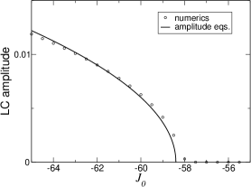
Figure 10: The bifurcation diagram for a supercritical Hopf bifurcation. Shown is the amplitude of the limit cycle as a function of the $0^{th}$ order spatial Fourier coefficient of the coupling $J(x)$. Open circles are from numerical simulation of Eq.(2) and solid lines show the solution from the amplitude equation, Eq.(16). The functions $\Phi$ and $J(x)$ as well as the input current $I$ and the delay $D$ are taken as in Fig. 7.

Figure 10 shows a typical bifurcation diagram (in this case $J_{1}=0$) for the Hopf bifurcation. Plotted is the amplitude of the limit cycle as a function of $J_{0}$ where symbols are from numerical simulation of Eq.(2) and the lines are from the amplitude equation, Eq.(18).

In the small delay limit ($D\to 0$) we can use the asymptotic values (11) to obtain, to leading order,

$$\mu+i\Omega=-\frac{(\frac{\pi}{2}+i)\Phi^{{}^{\prime}}}{1+\frac{\pi^{2}}{4}},$$ (19a)

$$\alpha+i\beta = -\frac{\chi}{(D\Phi^{\prime})^{3}}\Bigg{(}\frac{11\pi-4}{20}\frac{(\Phi^{{}^{\prime\prime}})^{2}}{\Phi^{{}^{\prime}}}-\frac{\pi\Phi^{{}^{\prime\prime\prime}}}{4}-i\bigg{[}\frac{11+\pi}{10}-\frac{\Phi^{{}^{\prime\prime\prime}}}{2}\bigg{]}\Bigg{)},$$ (19b)

where we have defined the quantity $\chi\equiv\pi^{3}/(8+2\pi^{2})$. Figure 11 shows a comparison of the full expressions for the coefficients of the amplitude equation, Eqs. (52-B.1.3) with the expressions obtained in the limit $D\to 0$, Eqs. (19a-19b). Again, the agreement is quite good, even up to $D=1$, especially for the real part of the cubic coefficient $\alpha$, which is of primary interest here.

Figure 11: Top: The real part of the linear coefficient $\mu$. Bottom: Minus the real part of the cubic coefficient $-\alpha$. Solid lines are from the full expressions Eq.(52-B.1.3) and dotted lines are the leading order terms in the small delay limit, Eqs. (19a-19b). The functions $\Phi$ and $J(x)$ as well as the input current $I$ are taken as in Fig. (7).

The asymptotic expression for the cubic coefficient $\alpha$, Eq.(19b), indicates that a subcritical limit cycle should occur for $\Phi^{{}^{\prime\prime\prime}}\Phi^{{}^{\prime}}/(\Phi^{{}^{\prime\prime}})^{2}>(11\pi-4)/(5\pi)$. This provides a simple criterion for determining whether or not a particular choice of the transfer function can generate oscillations which are bistable with the SU state. In fact, it is a difficult condition to fulfill given a sigmoidal-like input-output function. For example, given a sigmoid of the form $\Phi(x)=\alpha/(1+e^{-\beta x})$, one finds that

$$\frac{\Phi^{{}^{\prime\prime\prime}}\Phi^{{}^{\prime}}}{(\Phi^{{}^{\prime\prime}})^{2}}=1-2\frac{e^{-3\beta x}}{(e^{-4\beta x}-2e^{-3\beta x}+e^{-2\beta x})}.$$ (20)

It is straightforward to show that the expression of the right hand side of Eq.(20) is bounded above by $1$. In fact, $-\infty\leq\Phi^{{}^{\prime\prime\prime}}\Phi^{{}^{\prime}}/(\Phi^{{}^{\prime\prime}})^{2}<1<(11-4\pi)/(5\pi)\sim 1.95$. Such a nonlinear transfer function will therefore always generate supercritical oscillations.

If the nonlinear transfer function is interpreted as the single-cell fI curve, which is common in the literature, then we can use the fact that cortical cells operate in the fluctuation-driven regime. In particular, the mean input current to cortical cells is too low to cause spiking. Rather, this occurs at very low rates due to fluctuations in the membrane voltage. Although the fI curve for spiking neurons in the supra-threshold regime is concave down and saturates, in the fluctuation-driven, sub-threshold regime the fI curve exhibits a smoothed out tail which is concave up. It has been shown that the sub-threshold portion of the fI curve of actual cells can be well fit by a function of the form $\Phi(x)=Ax^{\gamma}$, where $\gamma>1$ (see e.g. [41, 36]). In this case

$$\frac{\Phi^{{}^{\prime\prime\prime}}\Phi^{{}^{\prime}}}{(\Phi^{{}^{\prime\prime}})^{2}}=1-\frac{1}{\gamma-1},$$

which again is bounded between $-\infty$ and $1$. This again rules out subcritical oscillations in the small delay limit.

Nonetheless, suitable functions $\Phi$ for generating subcritical oscillations can be contrived, as shown in Fig. 12 A. Numerical simulation of Eq.(2) indeed reveals a subcritical bifurcation in this case (see Fig. 12 B). However, this type of transfer function does not seem consistent with the interpretation of $\Phi$ as a single-cell fI curve, nor with that of $\Phi$ as a cumulative distribution of activation, i.e. a sigmoid. This strongly suggests that delay-driven oscillations in networks of spiking neurons will be generically supercritical.

Figure 12: A. An example of a function $\Phi(x)$ for which subcritical oscillations are possible. The dotted curve indicates the range of the function $\Phi$over which oscillations are subcritical. B. A bifurcation diagram for subcritical oscillations when the function $\Phi(x)$ is the same as in panel A. Open circles: the limit cycle amplitude computed numerically as a function of $J_{0}$. Here $D=0.1$ and the critical coupling is $\bar{J}_{0}=-15.89$. The fixed point is held at $R=0.1$ and thus the value of $x$ in panel A is close to 0.1 ($x+x^{3}=0.1$).

4.3 Turing-Hopf Bifurcation

4.3.1 Network simulations

As shown previously in [1], given an inverted Mexican-hat connectivity for which inhibition dominates locally, fast waves may emerge in networks of spiking neurons. This is illustrated in Fig.13A, where raster plots of three networks are shown with the degree of spatial modulation increasing from top to bottom.

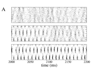
Figure 13: (Color online) Standing waves in a spiking network with inverted Mexican-hat connectivity with $p_{0}^{E}=p_{0}^{I}=0.2$, $p_{1}^{E}=0$ and $p_{2}^{E,I}=0$ (see Eq.(48) in the Appendix A) and $g_{E}=0.01$, $g_{I}=0.028$. The rate of the external Poisson inputs is $\nu_{ext}=5000$Hz and $g_{ext}=0.001$. A: Raster plots of spiking activity for three simulations with increasing spatial modulation of the connection probability between neurons. From top to bottom: $p_{1}^{I}=0.15$, $0.17$ and $0.20$. B: Top: The profile of activity in the three simulations averaged over 2500ms. The color code is black $p_{1}^{I}=0.15$, red $0.17$ and blue $0.2$. Bottom: The autocorrelation function of the firing rate averaged over all neurons in each simulation. Note that the instantaneous firing rate itself is not shown here.

Additionally, Fig. 13B (top) shows a spatial profile of the network activity averaged over 2500 ms for the three networks, while the bottom panel shows the autocorrelation function (AC) of the network firing rate for the three cases (same color scheme). Note that for small inhibitory spatial modulation $p_{1}^{I}$ (black curve) the profile is essentially flat while the AC exhibits an initial peak and dip, but an absence of multiple peaks which would indicate fast oscillations. As $p_{1}^{I}$ is increased (red curve), the profile remains flat but the AC clearly exhibits periodic peaks indicating that fast oscillations are present in the firing rate. The corresponding raster plot in the middle panel of Fig. 13 shows intermittent standing wave patterns which emerge and later disappear giving rise to a new pattern with a different spatial orientation (not shown). This explains why the time average of this spatial profile becomes flat. Finally, for strong enough spatial modulation, a stationary standing wave pattern is seen in Fig. 13A (bottom). In this case the time-averaged spatial profile shown in Fig. 13B (top, blue) shows two distinct maxima, whereas the AC indicates fast oscillations in the firing rate.

Extensive simulations with such a cosine connectivity always yielded standing wave patterns for various choices of synpatic weights and input rates (not shown). We seek to understand why this is so, and if delay-driven traveling wave patterns can also be seen in network numerical simulations. To this end we study the emergence of fast oscillations in the rate equation.

4.3.2 Rate equation

There is a spatially inhomogeneous oscillatory instability with frequency $\omega$ given by Eq.(9a). This occurs for a value of the $k^{th}$ spatial Fourier mode of the connectivity given by Eq.(9b), while we assume that all other Fourier modes are sufficiently below their critical values to avoid additional instabilities. Without loss of generality we assume $k=1$.

We expand the parameters $J_{1}$, $I$ and $r$ as in Eqs. (12,13,14) and define the slow time Eq. (15). The linear solution consists of leftwards and rightwards traveling waves with an amplitude which we allow to vary slowly in time, i.e. $r_{1}=A(T)e^{i\omega t+ix}+B(T)e^{-i\omega t+ix}+c.c.$. Carrying out a weakly nonlinear analysis to third order in $\epsilon$ leads to the coupled amplitude equations

$$\partial_{T}A=(\mu+i\Omega)\Delta J_{1}A+(a+ib)|A|^{2}A+(c+id)|B|^{2}A,$$ (21a)

$$\partial_{T}B=(\mu-i\Omega)\Delta J_{1}B+(a-ib)|B|^{2}B+(c-id)|A|^{2}B,$$ (21b)

where the coefficients $(a+ib)$, $(c+id)$ and $(\mu+i\Omega)$ are given by the Eqs. (54,55,52), respectively.

In the small delay limit ($D\to 0$) we can use the asymptotic values (11) to obtain, to leading order,

$$a+ib=\frac{\chi(\frac{\pi}{2}+i)}{(D\Phi^{{}^{\prime}})^{3}}\Bigg{(}\frac{J_{0}(\Phi^{{}^{\prime\prime}})^{2}}{1-\Phi^{{}^{\prime}}J_{0}}+\frac{\Phi^{{}^{\prime\prime\prime}}}{2}\Bigg{)},$$ (22a)

$$c+id=\frac{\chi(\frac{\pi}{2}+i)}{(D\Phi^{{}^{\prime}})^{3}}\Bigg{(}\frac{J_{0}(\Phi^{{}^{\prime\prime}})^{2}}{1-\Phi^{{}^{\prime}}J_{0}}+\Phi^{{}^{\prime\prime\prime}}+\frac{J_{2}(\Phi^{{}^{\prime\prime}})^{2}}{1-\Phi^{{}^{\prime}}J_{2}}\Bigg{)},$$ (22b)

where $\chi\equiv\pi^{3}/(8+2\pi^{2})$. Figure 14 shows a comparison of the full expressions (solid lines) for the real parts of the cubic and cross-coupling coefficients $a$ and $c$ with the asymptotic expressions above (dotted lines).

Figure 14: Top: The real part of the cubic coefficient $a$. Bottom: The real part of the cross-coupling coefficient $c$. Solid lines are from the full expressions Eq.(54-55) and dotted lines are the leading order terms in the small delay limit, Eqs. (22a-22b). The functions $\Phi$ and $J(x)$ as well as the input current $I$ are taken as in Fig. (7).

4.3.3 Wave solutions and their stability.

The equations (21a) and (21b) admit solutions of the form $(A,B)=(\mathcal{A}e^{i\theta_{A}},\mathcal{B}e^{i\theta_{B}})$, where the amplitudes $\mathcal{A}$ and $\mathcal{B}$ obey

$$\dot{\mathcal{A}}=\mu\Delta J_{1}\mathcal{A}+a\mathcal{A}^{3}+c\mathcal{B}^{2}\mathcal{A},$$ (23a)

$$\dot{\mathcal{B}}=\mu\Delta J_{1}\mathcal{B}+a\mathcal{B}^{3}+c\mathcal{A}^{2}\mathcal{B}.$$ (23b)

Traveling waves: Leftward and rightward traveling waves in Eqs. (23a) and (23b) are given by $(\mathcal{A}_{TW},0)$ and $(0,\mathcal{A}_{TW})$ respectively, where $\mathcal{A}_{TW}=-\mu\Delta J_{1}/a$. The stability of traveling waves can be determined with the ansatz $(\mathcal{A},\mathcal{B})=(\mathcal{A}_{TW},0)+(\delta\mathcal{A},\delta\mathcal{B})e^{\lambda t}.$ The resulting eigenvalues are $\lambda_{1}=-2\mu\Delta J_{1}$ and $\lambda_{2}=-\mu\Delta J_{1}(c/a-1)$.

Standing waves: Standing waves in Eqs. (23a) and (23b) are given by $(\mathcal{A}_{SW},\mathcal{A}_{SW})$, where $\mathcal{A}_{TW}=-\mu\Delta J_{1}/(a+c)$. The stability of standing waves can be determined with the ansatz $(\mathcal{A},\mathcal{B})=(\mathcal{A}_{SW},\mathcal{A}_{SW})+(\delta\mathcal{A},\delta\mathcal{B})e^{\lambda t}.$ The resulting eigenvalues are $\lambda_{1}=-2\mu\Delta J_{1}$ and $\lambda_{2}=-2\mu\Delta J_{1}(a-c)/(a+c)$.

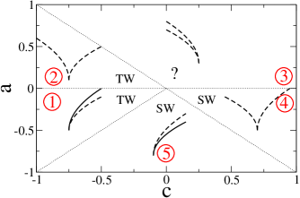
Figure 15: The existence and stability of traveling and standing waves as a function of the cubic and cross-coupling coefficients $a$ and $c$ given by Eqs. (22a,22a) and, in the small delay limit, by Eq. (24). In each sector of parameter space a representative bifurcation diagram is shown. Supercritical (subcritical) solutions are shown growing from left to right (right to left). Stable (unstable) solutions are given by solid (dashed) lines. Also indicated in each sector is the type of solution which will be seen numerically. A question mark is placed wherever the type of stable solution cannot be determined through a weakly nonlinear analysis.

The existence and stability of small-amplitude waves as described above is completely determined by the values of the cubic and cross-coupling coefficients $a$ and $c$. This is illustrated in Fig. 15, where the parameter space is divided into five sectors. In each sector the type of solution which will be observed numerically is indicated where known, and otherwise a question mark is placed. Illustrative bifurcation diagrams are also given. Specifically, in the region labeled 1 (red online), the SW solution is supercritical and unstable while the TW solution is supercritical and stable. TW will therefore be observed. In the region labeled 2, the SW solution is supercritical and unstable while the TW solution is subcritical. Finite-amplitude TW are therefore expected to occur past the bifurcation point. In the region labeled 3, both solution branches are subcritical, indicating that the analysis up to cubic order is not sufficient to identify the type of wave which will be observed. In the region labeled 4, TW are supercritical and unstable while SW are subcritical. Finite amplitude SW are therefore expected past the bifurcation point. In the region labeled 5, the TW solution is supercritical and unstable while the SW solution is supercritical and stable. SW will therefore be observed.

Performing the small delay limit we find, from Eqs. (22a,22b), that

$$a=c-\frac{\pi}{2}\frac{\chi}{(D\Phi)^{3}}\Bigg{(}\frac{\Phi^{{}^{\prime\prime\prime}}}{2}+\frac{J_{2}(\Phi^{{}^{\prime\prime}})^{2}}{1-\Phi^{{}^{\prime}}J_{2}}\Bigg{)}.$$ (24)

From Fig. 15 we can see that the nature of the solution seen will depend crucially on the sign of the second term of the right-hand side of Eq.(24). In particular, the diagonal $a=c$ divides the the parameter space into two qualitatively different regions. Above this line TWs are favored while below it SWs are favored. In the small delay limit, Eq.(24) indicates that the balance between the third derivative of the transfer function $\Phi^{{}^{\prime\prime\prime}}$ and the second spatial Fourier mode of the connectivity kernel will determine whether TW or SW are favored.

For sigmoidal transfer functions, the third derivative changes sign from positive to negative already below the inflection point, while for expansive power-law nonlinearities, which fit cortical neuronal responses quite well in the fluctuation-driven regime, the third derivative is positive if the power is greater than 2 and is negative otherwise. The contribution of this term therefore will depend on the details of the neuronal response. In simulations of large networks of conductance-based neurons in the fluctuation-driven regime in which $J_{2}$ was zero, the standing wave state was always observed, indicating a $\Phi^{{}^{\prime\prime\prime}}>0$ [1, 2].

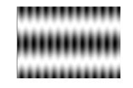
A		B
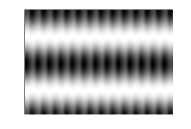
	time		time
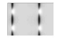
C		D
	time		time

Figure 16: Examples of wave solutions from numerical simulation of Eq.(2). The functions $\Phi$ and $J(x)$ as well as the input current $I$ and the delay $D$ are taken as in Fig. 7, with $J_{1}=-120$. A. Supercritical standing waves: $J_{0}=-40$ and 5 units of time are shown. B. Supercritical standing waves: $J_{0}=-9$ and 5 units of time are shown. C. Subcritical standing waves: $J_{0}=-5$ and 40 units of time are shown. D. Subcritical traveling waves: $J_{0}=0$ and 5 units of time are shown.

The phase diagram for $J_{2}=0$, Fig. 7, clearly shows the dominance of the SW solution, indicating $\Phi^{{}^{\prime\prime\prime}}>0$ for the parameter values chosen. Specifically, for values of $J_{0}<-6.3$, supercritical standing waves are stable (see region 5 in Fig. 15). Figures 16 A and 16 B show supercritical SW patterns for $J_{0}=-40$ and $J_{0}=-9$, respectively. For $-6.3<J_{0}<-2.6$, TW are supercritical and unstable while SW are subcritical [see region 4 in Fig. 15]. An example of subcritical SW is shown in Fig. 16 C. For $-2.6<J_{0}<3.58$, both SW and TW are subcritical (see region 3 in Fig. 15). Numerical simulations reveal TW patterns in this region (see an example in Fig. 16 D). In the region where SW are subcritical there is a small sliver in $(J_{0},J_{1})$ where the SW state is bistable with a TW state (TW/SW in the phase diagram). This TW branch most likely arises in a secondary bifurcation slightly below the Turing-Hopf bifurcation line. There is also a small region of bistability between large amplitude TW and the spatially uniform high activity state (TW/HA in the phase diagram Fig. 7).

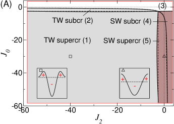
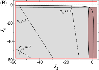
Figure 17: (Color online) A. Phase diagram for waves as a function of the zeroth and second spatial Fourier coefficients of the connectivity kernel. The dark-shaded region indicates SW, whereas the light shaded region indicates TW. Red lines indicate boundaries for primary instabilities of $J_{0}$ and $J_{2}$ given by Eqs. (8-9b). Solid stability lines for waves are from Eqs. (54-55) while the dashed line are from the asymptotic expressions (22a-22b). Here $\bar{J}_{1}=-58.4$. The function $\Phi$ as well as the input current $I$ and the delay $D$ are taken as in Fig. 7. Insets: example connectivity patterns corresponding to the values of $J_{0}$ and $J_{2}$ marked by the square and triangle respectively. B. The same phase diagram as in A, now showing where various types of ’difference-of-Gaussian’ connectivities, Eq. (25), would lie. Each dotted line indicates the border of a region in which the standard deviations of the excitatory and inhibitory connectivities are below a certain threshold (0.7, 1.0 and 1.5, respectively). Relatively narrow connectivities compared to the system size will always generate TW solutions. See text for details.

Thus for $\Phi^{{}^{\prime\prime\prime}}>0$ and with a simple cosine connectivity, SW arise for most values of $J_{0}$. However, adding a non-zero $J_{2}$ can lead to the TW solution winning out. The phase diagram of wave states as a function of $J_{0}$ and $J_{2}$ is shown in Fig. 17 A. In Fig. 17 A, the light shaded region indicates values of $J_{0}$ and $J_{2}$ for which TW are expected, whereas SW are expected in the dark shaded region. In the unshaded region, both TW and SW are subcritical and the solution type is therefore not determined by the analysis up to cubic order. These regions, delimited by the solid lines, were determined by numerically evaluating the real parts of the full expressions for the cubic and cross-coupling coefficients, Eqs. (54-55). Each region is furthermore numbered according to the existence and stability of the TW and SW solution branches as shown in Fig. 15. The dashed lines show the approximation to the solid lines given by the asymptotic formulas (22a-22b). The set of allowable values for $J_{0}$ and $J_{2}$ is bounded by the conditions (8-9b) corresponding to steady or oscillatory linear instabilities. These stability conditions are shown by the horizontal and vertical bounding lines (red online). All parameter values are as in Fig. 7.

From Fig. 17 we can now understand the discrepancy between the analytical results in [1] using a rate equation with a linear threshold transfer function, which predicted TW, and network simulations, which showed SW. Specifically, given a nonlinear transfer function with $\Phi^{{}^{\prime\prime\prime}}>0$, then with a simple cosine coupling SW are predicted over almost the entire range of allowable $J_{0}$ (dark shaded region for $J_{2}=0$). The nonlinear transformation of inputs into outputs is thus crucial in determining the type of wave solution. The choice of a threshold linear transfer function results in the second and all higher order derivatives being zero. In this sense it produces degenerate behavior at a bifurcation point, and by continuation of the solution branches, in a finite region of the phase diagram.

4.3.4 ’Difference-of-Gaussian’ connectivities

We have shown that varying $J_{0}$ can change the nature of the bifurcation, e.g. supercritical to subcritical, while varying $J_{2}$ can switch the solution type, e.g. from SW to TW. As an example of a functional form of connectivity motivated by anatomical findings, e.g. [42], we consider a difference of Gaussians, written as

$$J(x)=\frac{J_{e}}{\sqrt{2\pi}\sigma_{e}}e^{-\frac{x^{2}}{2\sigma_{e}^{2}}}-\frac{J_{i}}{\sqrt{2\pi}\sigma_{i}}e^{-\frac{x^{2}}{2\sigma_{i}^{2}}}.$$ (25)

In this case, one finds that the Fourier coefficients are

$$J_{k}=J_{e}e^{-k^{2}\sigma_{e}^{2}/2}f(k,\sigma_{e})-J_{i}e^{-k^{2}\sigma_{i}^{2}/2}f(k,\sigma_{i}).$$ (26)

where $f(k,\sigma_{e,i})=\text{Re}[\mbox{Erf}((\pi/\sigma_{e,i}+ik^{2})/\sqrt{2})]/\pi$. Once $J_{1}$ has been fixed at the critical value for the onset of waves, from Eq.(26) it is straightforward to show that $J_{0}=-pJ_{2}+q$ where both $p$ and $q$ are constants which depend on $\sigma_{e}$ and $\sigma_{i}$, the widths of the excitatory and inhibitory axonal projections respectively. Thus a difference-of-Gaussian connectivity, constrains the possible values of $J_{0}$ and $J_{2}$ to lie along a straight line for fixed connectivity widths. This is illustrated in Fig. 17B where three dashed lines are superimposed on the phase diagram, corresponding to the values $\sigma_{e,i}=(1.5,1.49)$; $\sigma_{e,i}=(1,0.99)$; and $\sigma_{e,i}=(0.7,0.69)$. Each of these lines is bounding a region to the left where $\sigma_{e}$ and $\sigma_{i}$ are less than $0.7$, $1.0$ and $1.5$ respectively. Given periodic boundary conditions with a system size of $2\pi$, a Gaussian with $\sigma=1.5$ is already significantly larger than zero for $x=\pi$ or $-\pi$. Thus, restricting ourselves to Gaussians which essentially decay to zero at the boundaries means that TW will always be observed. The same holds true for qualitatively similar types of connectivity.

4.3.5 Classes of waves in Network Simulations

Our analytical results concerning waves from the rate equation Eq.(2) predict that a connectivity with a sufficiently strong second Fourier component with a negative amplitude will lead to traveling waves (see the phase diagram in Fig. 17(A)).

Here we have confirmed this prediction performing numerical simulations of the network of spiking neurons described in the Appendix A. Indeed, Fig. 18 shows that the addition of the second spatial Fourier component to the inhibitory connections converts standing waves (SW) into travelling waves (TW).

Figure 18: The transition from (A) standing to (B) travelling waves in a network of conductance-based neurons takes place by increasing the second Fourier mode of the synaptic connectivity $p_{2}^{I}$. (A) $p_{2}^{I}=0$, (B) $p_{2}^{I}=0.1$. Remaining parameters: $p_{0}^{E,I}=p_{1}^{I}=0.2$, $p_{1,2}^{E}=0$, $g_{E}=0.01$, $g_{I}=0.028$, $g_{ext}=0.001$mS ms/cm², and $\nu_{ext}=5000$Hz.

5 Bifurcations of codimension 2

For certain connectivity kernels we may be in the vicinity of two distinct instabilities. This is the case for certain Mexican hat connectivities (OU and SB) and certain inverted Mexican hat connectivities (OU and SW/TW). Although two instabilities will co-occur only at a single point in the phase diagram Fig. 7, i.e. $J_{0}$ and $J_{1}$ are both at their critical values, the competition between these instabilities may lead to solutions which persist over a broad range of connectivities. This is the case here. We can investigate this competition once again using a weakly nonlinear approach. The main results of this section are summarized in table 1.

5.1 Hopf and Turing-Hopf bifurcations

Here we consider the co-occurrence a spatially homogeneous oscillation and a spatially inhomogeneous oscillation (OU and SW/TW), both with frequency $\omega$ given by Eq.(9a). This instability occurs when the zeroth and $k^{th}$ spatial Fourier mode of the connectivity both satisfy the relation, Eq.(9b), while we assume that all other Fourier modes are sufficiently below their critical values to avoid additional instabilities. Without loss of generality we take $k=1$ for the SW/TW state.

We expand the parameters $J_{0}$, $J_{1}$, $I$ and $r$ as in Eqs. (12,13,14), and define the slow time (15). The linear solution consists of homogeneous, global oscillations, leftwards and rightwards traveling waves with amplitudes which we allow to vary slowly in time, i.e. $r_{1}=H(T)e^{i\omega t}+A(T)e^{i\omega t+ix}+B(T)e^{-i\omega t+ix}+c.c.$. Carrying out a weakly nonlinear analysis to third order in $\epsilon$ leads to the coupled amplitude equations

$$\partial_{T}H = (\mu+i\Omega)\Delta J_{0}H$$

$$+2(\alpha+i\beta)[(\frac{|H|^{2}}{2}+|A|^{2}+|B|^{2})H+H^{*}AB^{*}],$$

$$\partial_{T}A = (\mu+i\Omega)\Delta J_{1}A+(a+ib)|A|^{2}A+(c+id)|B|^{2}A$$ (27b)

$$+(\alpha+i\beta)[2|H|^{2}A+H^{2}B],$$

$$\partial_{T}B = (\mu-i\Omega)\Delta J_{1}B+(a-ib)|B|^{2}B+(c-id)|A|^{2}B$$ (27c)

$$+(\alpha-i\beta)[2|H|^{2}B+H^{*2}A],$$

where $\alpha+i\beta$, $a+ib$ and $c+id$ are given by Eqs. (B.1.3,54,55), respectively. The overbar in $H^{*}$ represents the complex conjugate.

5.1.1 Solution types and their stability

Eqs. (27-27c) admit several types of steady state solutions including oscillatory uniform solutions (OU), traveling waves (TW), standing waves (SW) and mixed mode oscillations/standing waves (OU-SW). The stability of these solutions depends on the values of the coefficients in Eqs. (27-27c). In addition, non-stationary solutions are also possible. Here we describe briefly some stationary solutions and their stability. For details see B.

Oscillatory Uniform (OU): The oscillatory uniform solution has the form $(H,A,B)=(\mathcal{H}e^{i\omega t},0,0)$ where

$$\mathcal{H} = \sqrt{\frac{-\mu\Delta J_{0}}{\alpha}},$$

$$\omega = \Big{(}\Omega-\frac{\beta\mu}{\alpha}\Big{)}\Delta J_{0}.$$

The OU state undergoes a steady instability along the line

$$\Delta J_{1}=\Delta J_{0}.$$ (28)

This stability line agrees very well with the results of numerical simulations of Eq.(2) [see the phase diagram Fig. 7].

Traveling Waves (TW): The traveling wave solution has the form $(H,A,B)$ = $(0,\mathcal{A}_{TW}e^{i\omega t},0)$ or $(0,0,\mathcal{A}_{TW}e^{-i\omega t})$, where

$$\mathcal{A}_{TW} = \sqrt{\frac{-\mu\Delta J_{1}}{a}},$$

$$\omega = \Big{(}\Omega-\frac{b\mu}{a}\Big{)}\Delta J_{1}.$$

The TW state undergoes an oscillatory instability along the line

$$\Delta J_{1}=\frac{a}{2\alpha}\Delta J_{0},$$ (29)

with a frequency

$$\bar{\omega}=\Big{(}\Omega(1-\frac{a}{2\alpha})+(b-2\beta)\frac{\mu}{2\alpha}\Big{)}\Delta J_{0}.$$

Standing Waves (SW): The standing wave solution has the form $(H,A,B)$ = $(0,\mathcal{A}_{SW}e^{i\omega t},\mathcal{A}_{SW}e^{-i\omega t})$, where

$$\mathcal{A}_{SW} = \sqrt{\frac{-\mu\Delta J_{1}}{(a+c)}},$$ (30)

$$\omega = \Big{(}\Omega-\frac{(b+d)}{(a+c)}\mu\Big{)}\Delta J_{1}.$$ (31)

An oscillatory instability occurs along the line

$$\Delta J_{1}=\frac{(a+c)}{4\alpha}\Delta J_{0},$$ (32)

with a frequency

$$\bar{\omega}=\sqrt{[\Omega(\frac{a+c}{4\alpha}-1)-\mu\frac{b+d-4\beta}{4\alpha}]^{2}-\mu^{2}\frac{\alpha^{2}+\beta^{2}}{4\alpha^{2}}}\Delta J_{0}.$$

A stationary instability occurs along the line

$$\Delta J_{1}=\Psi\Delta J_{0},$$ (33)

where

$$\Psi=\frac{-k_{2}+\sqrt{k_{2}^{2}-4k_{1}k_{3}}}{2k_{1}},\\$$ (34)

$$k_{1}=\Big{[}\Omega-\mu\frac{(b+d-4\beta)}{(a+c)}\Big{]}^{2}+\mu^{2}\frac{(12\alpha^{2}-4\beta^{2})}{(a+c)^{2}},$$

$$k_{2}=-8\mu^{2}\frac{\alpha}{(a+c)}-2\Omega^{2}+2\Omega\mu\frac{(b+d-4\beta)}{(a+c)},$$

$$k_{3}=\mu^{2}+\Omega^{2}.$$

For Eq. (2) with the parameters used to generate the phase diagram Fig. 7, we find that the stationary instability precedes the oscillatory one and that $\Psi\sim 0.6$. This agrees well with the numerically determined stability line near the co-dimension 2 point in the diagram 7.

Mixed Mode: We can study the mixed mode solutions in Eqs. (27-27c) by assuming an ansatz

$$(H,A,B)=(\mathcal{H}e^{i\theta},\mathcal{A}e^{i\psi_{A}},\mathcal{B}e^{-i\psi_{B}}),$$ (35)

which leads to four coupled equations [see (B)]. We do not study the stability of mixed mode solutions in this work.

5.1.2 A simple example

We now turn to a simple example in order to illustrate the two main types bifurcation scenarios that can arise when small amplitude waves and oscillations interact in harmonic resonance.

i. Bistability: Here we take the parameters . Given these parameter values one finds, from the analysis above, that the oscillatory uniform state has an amplitude $\mathcal{H}=1$ and destabilizes along the line $\Delta J_{1}=-1$. The standing wave solution (traveling waves are unstable [see Fig. 15] has an amplitude $\mathcal{A}_{SW}=\sqrt{-\Delta J_{1}}$ which undergoes a steady bifurcation to the oscillatory uniform state at $\Delta J_{1}=-1/2$. Both solutions are therefore stable in the region $-1<\Delta J_{1}<-1/2$. This analysis is borne out by numerical simulation of Eqs. (27-27c) [see Fig. 19a]. Solid and dotted lines are the analytical expressions for the stable and unstable solution branches respectively (red is OU and black is SW). Circles are from numerical simulation of the amplitude equations (27-27c).

Note that this scenario is the relevant one for the phase diagram shown in Fig. 7. That is, we find there is a region of bistability between the OU and SW solutions, bounded between two lines with slope $\sim 0.6$ and $1$ respectively.

ii. Mixed Mode: Here we consider the parameters . Given these parameter values one finds that the oscillatory uniform state has an amplitude $\mathcal{H}=1$ and destabilizes along the line $\Delta J_{1}=-1$. The standing waves solution has an amplitude $\mathcal{A}_{SW}=\sqrt{-\Delta J_{1}/8}$ (traveling waves are again unstable) which undergoes an oscillatory instability at $\Delta J_{1}=-2$. The mixed-mode solution is given by

$$\mathcal{H} = \frac{4+\Delta J_{1}(2-\cos{\phi}-\sin{\phi})}{4-(2-\cos{\phi}-\sin{\phi})^{2}},$$ (36a)

$$\mathcal{A}_{SW} = \frac{\Delta J_{1}+(2-\cos{\phi}-\sin{\phi})}{8-2(2-\cos{\phi}-\sin{\phi})^{2}},$$ (36b)

$$1 = \Delta J_{1}(1-4\cos{\phi}-2\sin{\phi}+2\sin{\phi}\cos{\phi})-4\cos{\phi}+8\cos{\phi}^{2}.$$ (36c)

Figure 19: Two typical bifurcation diagrams for the case of harmonic resonance between small-amplitude oscillations and small-amplitude standing waves. A: Here oscillations and standing waves are bistable for $-1<\Delta J_{1}<-1/2$. $\Delta J_{0}=-1$, $\alpha=-1$, $a=-1$, $b=c=d=\beta=\Omega=0$, $\mu=-1$. B: Here the standing wave solution loses stability to an oscillatory mixed-mode solution at $\Delta J_{1}=-2$. At $\Delta J_{1}\sim-1.75$ a steady mixed-mode solution arises in a saddle-node bifurcation and continuously approaches the oscillatory pure-mode solution at $\Delta J_{1}=-1$. Parameters are $a=-8$, $\beta=1$, $\alpha=-1$, $\mu=-1$, $b=c=d=\Omega=0$. The phase $\phi$ of the mixed-mode solution is not shown.

It is easy to show that for $\Delta J_{1}\to-1$ the mixed mode amplitudes approach $(\mathcal{H},\mathcal{A}_{SW})=(1,0)$ and the phase $\phi\to 0$. The mixed-mode solution thus bifurcates continuously from the oscillatory pure mode. Figure 19b shows the corresponding bifurcation diagram where solid and dotted lines are the analytical expressions for the solution branches and symbols are from numerical simulation of Eqs. (27-27c). As $\Delta J_{1}$ increase from the left we see that the SW solution indeed undergoes an oscillatory instability at $\Delta J_{1}=-2$ leading to an oscillatory mixed-mode solution indicated by small circles (the maximum and minimum amplitude achieved on each cycle is shown). This oscillatory solution disappears in a saddle-node bifurcation, giving rise to a steady mixed-mode solution whose amplitude is given by Eq.(36a- 36c). This steady mixed-mode solution bifurcates from the pure oscillatory mode at $\Delta J_{1}=-1$ as predicted.

5.1.3 Summary

The interaction between the oscillatory uniform state and waves may lead to mixed mode solutions or bistability. The OU state always destabilizes along the line $J_{1}=J_{0}$, irrespective of parameter values or the choice of $\Phi$ or $J(x)$. This result from the weakly nonlinear analysis, agrees with numerical simulations of Eq.(2) over the entire range of values of $J_{0}$ and $J_{1}$ used in the phase diagram, Fig. 7 and appears to be exact. Depending on the value of $J_{2}$, supercritical TW or supercritical SW will be stable near the codimension 2 point. In the case of TW, the slope of the stability line is one half the ratio of the cubic coefficient of waves to that of oscillations. In the small delay limit this expression can be simplified to

$$\frac{a}{2\alpha}\sim\frac{\pi}{4}\frac{\Big{(}\frac{(\Phi^{{}^{\prime\prime}})^{2}}{\Phi^{{}^{\prime}}}-\frac{\Phi^{{}^{\prime\prime\prime}}}{2}\Big{)}}{\Big{(}\frac{(11\pi-4)}{20}\frac{(\Phi^{{}^{\prime\prime}})^{2}}{\Phi^{{}^{\prime}}}-\frac{\pi\Phi^{{}^{\prime\prime\prime}}}{4}\Big{)}},$$ (37)

which depends only on shape of the transfer function $\Phi$. For the parameter values used in the phase diagram Fig. 7 this yields a line with slope close to one half. Thus TW and OU are expected to be bistable in the wedge between $\Delta J_{1}=\Delta J_{0}/2$ and $\Delta J_{1}=\Delta J_{0}$. In the case of SW, the slope of the stability line is a complicated function of the shape of $\Phi$ and the second Fourier coefficient $J_{2}$. For the parameter values used in the phase diagram Fig. 7 the slope is close to 0.6. Therefore the OU and SW states are bistable in the wedge between $\Delta J_{1}=0.6\Delta J_{0}$ and $\Delta J_{1}=\Delta J_{0}$.

5.1.4 Network simulations

Given that network simulations robustly reveal standing wave patterns, we would expect to find either mixed-mode SW-OU or bistability between SW and OU. As we have shown previously, e.g. [1], there is a region of bistability between SW and OU in network simulations for strongly modulated inhibitory connectivity. Here we show additional network simulations that suggest this bistable region is in the vicinity of the codimension two point, i.e. it is a bistability between the OU and SW states arising via primary bifurcations of the unpatterned state.

Figure 20: Bistability between SW and OU states in an inhibitory network with $p_{I}(r)=0.4+0.2\cos{r}$, where $r$ is the distance between neurons, $\nu_{ext}=4500$Hz, and $g_{I}=0.1$mS$\cdot$ms/cm². This is, the only network simulation for which an explicit delay has been added of $\delta=0.5$ms. Removing the explicit delay for these parameter values eliminates the bistability. Parameter values are identical for both simulations. In the simulation shown in the bottom raster a hyperpolarizing current of $I_{app}=-5.0\mu$A/cm² was injected into cells 1-1000 for 30ms at time $t=400$ms, switching the state from OU to SW.

Figure 20 shows two rasters from simulations of a purely inhibitory network with strongly spatially modulated connectivity. The top raster shows 300 milliseconds of activity in which homogeneous oscillations are clearly observable. In the bottom raster, the network is started from the precisely the same initial condition, but a hyperpolarizing input current is applied to neurons 1 to 1000 from t=400 to t=430ms. The network activity clearly switches to a SW state in response to this input. The SW state persists for as long as simulations were carried out (10sec). The network thus exhibits bistability between the OU and SW states.

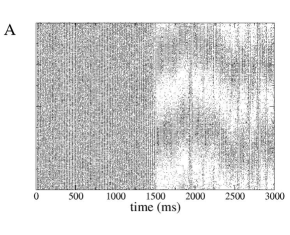
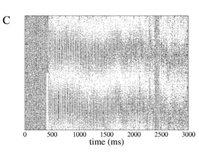
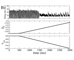
Figure 21: Increasing the strength of recurrent excitatory connections drives the system out of the bistable regime and into a SW state. A: A raster plot of 3 seconds of simulation. For the first 500ms the simulation is identical to that shown in the top panel of Fig.20. Thereafter the weights of the recurrent excitatory synaptic are slowly increased while the external drive is slowly decreased so as to maintain stable mean firing rates. There is a spontaneous destabilization of the OU state to a SW state around $t=1500$ms. B: The network firing rate for the simulation shown in A (top), the time course of the excitatory synaptic weights (middle) and external drive (bottom). C: For the first 500ms the simulation is identical to that shown in the bottom panel of Fig.20, i.e. there is a hyperpolarizing current injected at time $t=400$ms which switches the state from OU to SW. Thereafter the weights of recurrent excitatory synapses are slowly increased while the external drive is slowly decreased so as to maintain stable mean firing rates. D: The network firing rate and time courses of the excitatory synaptic weights and external drive, as in B.

In order to determine if this region of bistability is related to the codimension 2 point, we adiabatically increased the recurrent excitatory connectivity in the network, thereby mimicking an increase in $J_{0}$ in the rate model. This is done by generating a network of both inhibitory and excitatory neurons with $p_{I}(r)=0.4+0.2\cos{r}$ and $p_{E}=0.2$. The weights of the inhibitory synapses are taken as $g_{I}=0.1$ while excitatory weights are allowed to vary. Specifically, $g_{E}=0$ for the first 500ms of the simulation and are then slowly increased according to $g_{E}(t)=1.0526\cdot 10^{-5}(t-500)$. At the same time we slowly decrease the external drive in order to maintain mean firing rates. Thus $\nu_{ext}=4500$ for the first 500ms and is then varied according to $\nu_{ext}=4500-0.158(t-500)$ thereafter. This particular functional form was determined empirically to keep the mean firing rates steady. Therefore, for the first 500ms of simulation time the network is equivalent to that shown in Fig. 20 while at later times the network is no longer purely inhibitory.

Carrying out such an adiabatic increase in the recurrent excitation should cause the network to cross the line of instability of the OU state, leading to stable SW. Thus, if we begin simulations in the OU state, they should destabilize at some point to SW while if we begin in the SW state they should persist. This is precisely what occurs. Fig.21A shows a raster plot of three seconds of simulation time begining in the OU state. A transition to the SW occurs around 1500ms. Fig.21B shows the network firing rate during these three seconds (top) as well as the time course of the excitatory synaptic weights and external drive (middle and bottom respectively). Note that the mean firing rate is relatively steady in the OU state indicating that the co-variation of the synaptic weights and external drive balance one another. Fig.21C and D analogously show the raster and firing rate of a simulation in which the network is switched into a SW state at $t=400$ms. Note that the SW state persists over the whole 3 sec. simulation.

5.2 Hopf and Turing bifurcations

We consider the co-occurrence of two instabilities: a spatially homogeneous oscillation and a spatially inhomogeneous steady solution. This occurs when the zeroth spatial Fourier mode of the connectivity satisfies the relation, Eq.(9b) and the $k_{th}$ spatial Fourier mode satisfies $J_{1}=1/\Phi^{{}^{\prime}}$, while we assume that all other Fourier modes are sufficiently below their critical values to avoid additional instabilities. Without loss of generality we take $k=1$ for the Turing instability.

We expand the parameters $J_{0}$, $J_{1}$, $I$ and $r$ as in Eqs. (12,13,14), and define the slow time (15). The linear solution consists of homogeneous, global oscillations and stationary, spatially periodic bumps with amplitudes which we allow to vary slowly in time, i.e. $r_{1}=H(T)e^{i\omega t}+A(T)e^{ix}+c.c.$. Carrying out a weakly nonlinear analysis to third order in $\epsilon$ leads to the coupled amplitude equations

$$\partial_{T}H=(\mu+i\Omega)\Delta J_{0}H+(\alpha+i\beta)|H|^{2}H+(\kappa+i\Lambda)|A|^{2}H,$$ (38a)

$$\partial_{T}A=\bar{\eta}\Delta J_{1}A+\Gamma|A|^{2}A+\sigma|H|^{2}A,$$ (38b)

where $\mu+i\Omega$, $\alpha+i\beta$, $\bar{\eta}$, $\Gamma$, $\kappa+i\Lambda$ and $\sigma$ are given by Eqs. (52,B.1.3,17a,17b, 71,72), respectively.

5.2.1 Solution types and their stability

Steady state solutions to Eqs. (38a,38b) include pure mode OU, pure mode SB and mixed mode solutions (OU-SB). We look at the stability of the OU and SB solutions in turn for the general case and then look specifically at the case of small delay in Eq.(2). Since the coupling in Eqs. (38a-38b) is only through the amplitudes we can simplify the equations by taking $(H,A)=(\mathcal{H}e^{i\theta},\mathcal{A}e^{i\phi})$ which yields

$$\dot{\mathcal{H}}=\mu\Delta J_{0}\mathcal{H}+\alpha\mathcal{H}^{3}+\kappa\mathcal{A}^{2}\mathcal{H},$$ (39a)

$$\dot{\mathcal{A}}=\eta\Delta J_{1}\mathcal{A}+\Gamma\mathcal{A}^{3}+\sigma\mathcal{H}^{2}\mathcal{A}.$$ (39b)

Oscillatory Uniform (OU): The uniform oscillations have the form $({\mathcal{H^{*}}},0)$ where

$$\mathcal{H}=\sqrt{-\frac{\mu\Delta J_{0}}{\alpha}}.$$

The linear stability of this solution can be calculated with the ansatz

$$(\mathcal{H},\mathcal{A})=({\mathcal{H^{*}}}+\delta\mathcal{H}e^{\lambda t},\delta\mathcal{A}e^{\lambda t}),$$

which yields the two eigenvalues

$$\lambda_{H}=-2\mu\Delta J_{0},$$ (40)

$$\lambda_{A}=\eta\Delta J_{1}+\frac{\mu\sigma}{\alpha}\Delta J_{0}.$$

If we assume a supercritical uniform oscillatory state then the first eigenvalue is always negative, while the second becomes positive along the line

$$\Delta J_{1}=\frac{\mu\sigma}{\eta\alpha}\Delta J_{0},$$ (41)

indicating the growth of a bump solution.

For Eq.(2) with the parameters used to generate the phase diagram Fig. 7, we find from Eq.(41) that the OU state destabilizes along the line $\Delta J_{1}\sim-0.026\Delta J_{0}$.

Stationary Bump (SB): The stationary bump solution has the form $(0,{\mathcal{A^{*}}})$ where

$$\mathcal{A}=\sqrt{-\frac{\eta\Delta J_{1}}{\Gamma}}.$$

The linear stability of this solution can be calculated with the ansatz

$$(\mathcal{H},\mathcal{A})=(\delta\mathcal{H}e^{\lambda t},{\mathcal{A^{*}}}+\delta\mathcal{A}e^{\lambda t}),$$

which yields the two eigenvalues

$$\lambda_{H}=\mu\Delta J_{0}-\frac{\eta\kappa}{\Gamma}\Delta J_{1},$$ (42)

$$\lambda_{A}=-2\eta\Delta J_{1}.$$

If we assume a supercritical stationary bump state then the second eigenvalue is always negative, while the first becomes positive along the line

$$\Delta J_{1}=\frac{\mu\Gamma}{\eta\kappa}\Delta J_{0},$$ (43)

indicating the growth of uniform oscillations.

For Eq.(2) with the parameters used to generate the phase diagram 7, we find from Eq.(43) that the SB state destabilizes along the line $\Delta J_{1}\sim-0.144\Delta J_{0}$.

Mixed Mode (OU-SB): The mixed-mode solution satisfies the following matrix equation

$$\left(\begin{array}[]{cc}\alpha&\kappa\\ \sigma&\Gamma\end{array}\right)\left(\begin{array}[]{c}\mathcal{H}^{2}\\ \mathcal{A}^{2}\end{array}\right)=-\left(\begin{array}[]{c}\mu\Delta J_{0}\\ \eta\Delta J_{1}\end{array}\right),$$

which yields

$$\mathcal{H}^{2}=\frac{-\mu\Gamma\Delta J_{0}+\eta\kappa\Delta J_{1}}{\alpha\Gamma-\sigma\kappa},$$ (44)

$$\mathcal{A}^{2}=\frac{\mu\sigma\Delta J_{0}-\eta\alpha\Delta J_{1}}{\alpha\Gamma-\sigma\kappa}.$$

We do not study the stability of the mixed-mode solution here.

Figure 22: Typical bifurcation diagrams for the competition between bumps and global oscillations. $\mu=-1$, $\Delta J_{0}=-1$, $\alpha=-1$, $\eta=1$, $\Gamma=-1$. A: $\kappa=-2$, $\sigma=-2$. The limit cycle and bump solutions are bistable in the range $1/2<\Delta J_{1}<2$. B: A mixed-mode solution is stable in the range $1/2<\Delta J_{1}<2$. $\kappa=-0.5$, $\sigma=-0.5$. Symbols are from simulation of the amplitude equations Eqs. (39a-39b) while lines are the analytical expressions.

5.2.2 A simple example

We once again illustrate the scenarios of bistability and mixed-mode solutions with a simple example.

i. Bistability : In this case, the limit cycle has an amplitude $\mathcal{H}=1$ and undergoes an instability at $\Delta J_{1}=2$. The bump solution has an amplitude $\mathcal{A}=\sqrt{\Delta J_{1}}$ and becomes unstable at $\Delta J_{1}=1/2$. The oscillatory and bump solutions are therefore bistable in the range $1/2<\Delta J_{1}<2$. This is borne out in numerical simulations of Eqs. (39a-39b) [see Fig. 22A]. Symbols are from numerical simulation (circles:limit cycle, squares:bump), while lines are analytical solutions.

ii.Mixed-mode : In this case, the limit cycle has an amplitude $\mathcal{H}=1$ and undergoes an instability at $\Delta J_{1}=1/2$. The bump solution has an amplitude $\mathcal{A}=\sqrt{\Delta J_{1}}$ and becomes unstable at $\Delta J_{1}=2$. The mixed-mode solution is stable in the range $1/2<\Delta J_{1}<2$ and has amplitudes $\mathcal{H}_{MM}=2\sqrt{(1-\Delta J_{1}/2)/3}$ and $\mathcal{A}=2\sqrt{(\Delta J_{1}-1/2)3}$. The corresponding bifurcation diagram is shown in Fig. 22B where symbols are from simulation of Eqs. (39a-39b) and lines are the analytical results.

5.2.3 Summary

Codim.-2 bifurcations	Solution types calculated	Instability boundaries
Hopf and Turing-Hopf	Oscillatory Uniform	$\Delta J_{1}=\Delta J_{0}$
	Travelling Waves	$\Delta J_{1}=a/(2\alpha)\Delta J_{0}$
	Standing Waves (osc.)	$\Delta J_{1}=(a+c)/(4\alpha)\Delta J_{0}$
	Standing Waves (stat.)	$\Delta J_{1}=\Psi\Delta J_{0}$
	Mixed-Mode	Not calculated
Hopf and Turing	Oscillatory Uniform	$\Delta J_{1}=(\mu\sigma)/(\eta\alpha)\Delta J_{0}$
	Stationary Bump	$\Delta J_{1}=(\mu\Gamma)/(\eta\kappa)\Delta J_{0}$
	Mixed-Mode (OU-SB)	Not calculated

Table 1: Some existing dynamical states that are present close to the codimension-2 bifurcations, and their corresponding instability boundaries Eqs. (28,29,32,33,41,43), except for the Mixed Mode solutions.

The interaction between the SB and OU states can lead to one of two scenarios. Either there is a region of bistability between bumps and oscillations, or there is a mixed-mode solution which, near the codimension-2 point at least, will consist of bumps whose amplitude oscillates in time, i.e. oscillating bumps (OB).

In the limit of small $D$ the instability lines for the OU and SB states in the vicinity of the codimension 2 point are given by the equations

$$\Delta J_{1} = -D\frac{\Big{(}\frac{(\Phi^{{}^{\prime\prime}})^{2}}{\Phi^{{}^{\prime}}}-\Phi^{{}^{\prime\prime\prime}}\Big{)}}{\Big{(}\frac{(11\pi-4)}{20}\frac{(\Phi^{{}^{\prime\prime}})^{2}}{\Phi^{{}^{\prime}}}-\pi\frac{\Phi^{{}^{\prime\prime\prime}}}{4}\Big{)}}\Delta J_{0},$$ (45)

$$\Delta J_{1} = -\frac{2}{\pi}D\frac{\Big{(}\frac{(\Phi^{{}^{\prime\prime}})^{2}}{\Phi^{{}^{\prime}}}-\frac{\Phi^{{}^{\prime\prime\prime}}}{2}-\frac{J_{2}(\Phi^{{}^{\prime\prime}})^{2}}{2(1-J_{2}\Phi^{{}^{\prime}})}\Big{)}}{\Big{(}\frac{(\Phi^{{}^{\prime\prime}})^{2}}{\Phi^{{}^{\prime}}}-\Phi^{{}^{\prime\prime\prime}}\Big{)}}\Delta J_{0}.$$ (46)

respectively. The slope of both of the stability lines is proportional to $D$, indicating that in the small $D$ limit any region of bistability or mixed mode solution will be limited to a narrow wedge close to the $J_{0}$ axis. Which scenario will be observed (bistability or mixed-mode) depends on the particular choice of $\Phi^{{}^{\prime}}$ and the value of the second spatial Fourier mode of the connectivity $J_{2}$. For the parameters values used to generate the phase diagram Fig. 7 the slopes are $\sim-0.026$ and $\sim-0.144$ for the OU and SB stability lines respectively, indicating a mixed mode solution.

5.2.4 Network simulations

As shown in [1], oscillating bump solutions can be found in networks of spiking neurons with Mexican-hat connectivity and strong inhibition. Here we have identified such oscillating bumps as arising via a bifurcation to mixed-mode OU and SB in the vicinity of the codimension-two point for homogeneous oscillations and Turing patterns. Fig.23 shows a sample raster from a numerical simulatiom simulation. The top panel shows a mixed-mode solution which drifts in time. The bottom panel is a blow-up of the raster for $500$ms$<t<700$ms where the fast oscillations are clearly visible.

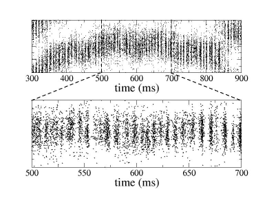
Figure 23: A mixed mode (OU/SB) solution in a network of spiking neurons with $p_{E}=0.2+0.1\cos{r}$, $p_{I}=0.2$, $g_{E}=0.1$, $g_{I}=0.28$, $\nu_{ext}=2000$ and $g_{ext}=0.01$. See text for details.

6 Conclusions

Our main objective in this paper was to understand in greater detail the dynamical states which arise in networks of spiking neurons. Specifically, we are interested in large networks of irregularly spiking neurons for which a reduced, phenomenological description in terms of mean firing rates is a reasonable approximation. This is the case, for example, if the connectivity is sparse and cross-correlations of the input currents to different cells are therefore weak. The particular form of the rate equation description is motivated by the observation of emergent fast oscillations in simulations of networks with dominant inhibition, e.g. [3]. The origin of these oscillations has been well studied in model networks and is due to an effective delay in neuronal interactions generated by the synaptic kinetics and single-cell dynamics [34, 35]. The dynamics of the mean firing rate of the resulting oscillatory states can be captured by a rate equation with an explicit time delay [1].

However, the rate equation considered previously did not agree entirely with network simulations. Specifically, it predicted a large region of traveling wave solutions while in the network simulations only standing waves were found to be stable. Our analysis here has shown that given a more realistic transfer function, i.e. sigmoidal or expansive power-law nonlinearity, the primary inhomogeneous oscillatory instability given a cosine connectivity will be to standing waves. This suggests that the standing wave states robustly observed in network simulations were due to the nonlinearity in the single cell fI curve, and that the rate model with threshold linear transfer function studied in [1] was not able to capture this effect.

We predicted further that altering the connectivity could stabilize the traveling wave state. Specifically, more realistic patterns of connectivity, such as Gaussian, affect the competition between traveling and standing waves through the second spatial Fourier mode. In the case of delay-driven waves, where the primary instability occurs only for strong inhibition, we show that the sign of the second mode will be negative and that in the limit of small delay this will always lead to traveling waves. This prediction is borne out in network simulations, see Fig.18.

We furthermore show that the bifuration to homogeneous oscillations is supercritical for standard choices of transfer functions, again sigmoidal and expansive power-law. This agrees with network simulations of conductance-based neurons we have conducted, and with the amplitude equation derived for a network of integrate-and-fire neurons [3].

It is more difficult to draw clear-cut conclusions regarding the dynamical states seen in the vicinity of the two codimension-two points we have studied: Hopf/Turing-Hopf and Hopf/Turing. In general there will either be a region of bistability between the two states which bifurcate via primary instabilities in the vicinity of the codimension-two point, or there will be one or several mixed-mode solutions. In network simulations we have shown examples of both: bistable OU/SW and mixed mode OU/SB. Many more complex dynamical states can be observed both in the rate model and the network simulations further from the primary bifurcations. Here we have chosen an analytical approach which is powerful enough to allow for arbitrary transfer functions and connectivity, but which is limited to the parameter space in the vicinity of the primary bifurcations. This is a complementary approach to that taken in [1], where a specific choice of transfer function and connectivity allowed for an analysis of several nonlinear states, even far from the primary bifurcations.

The approach we have taken in this paper is similar in spirit to that of Curtu and Ermentrout [33]. In that work, they study an extension of a rate model with adaptation proposed by Hansel and Sompolinsky [32]. As in our work here, they allow for a generic transfer function and generic connectivity and derive amplitude equations for the primary Turing and Turing-Hopf bifurcations which occur. Thus both adaptation and the effective delay in neuronal interactions can lead to waves. However, the waves in these two cases arise via distinct physiological mechanisms and can exhibit very different propagation velocities.

In the case of adaptation, waves arise given patterns of synaptic connectivity which, in the absence of adaptation would lead to the emergence of bump states, i.e. a Turing instability. These tend to be Mexican-hat like connectivities. In the presence of adaptation, stationary bump states may destabilize since the peak of activity is preferentially suppressed compared to activity at the edge of the bump. As a result the bump begins to move via a symmetry-breaking bifurcation, generally leading to traveling waves. This only occurs if the adaptation is significantly strong, i.e. above a critical threshold. In a two-population model with adaptation studied in [33], the frequency of the waves was shown to be proportional to the square root of the difference between the strength of adaptation and a critical value below which no bifurcation is possible. Thus the resulting waves can be arbitrarily slow depending on the strength of adaptation.

In the case of rate equations with delay, a Turing-Hopf instability occurs only for connectivities which are strongly inhibitory locally, i.e. inverted Mexican-hat connectivities. A transient perturbation which increases the firing rate locally will, after a delay, strongly self-inhibit while increasing the firing rate of more distant neurons. The process then repeats, leading to a propagation of activity. The frequency of such waves is clearly related to the delay, which itself depends on the synaptic time constants as well as the spike generation currents [34, 35].

Finally, we have tried to emphasize the importance of fixed delays in shaping the dynamics described by Eq.(2) and by extension in networks of spiking neurons. Nonetheless both fixed and conduction delays are present in neuronal systems and are roughly of the same order of magnitude in a small patch of cortex of $\sim 1$mm in extent. It remains to be studied how these delays interact to shape patterns of spontaneous activity.

Appendix A The network of spiking neurons

In this appendix we describe the network of conductance-based neurons used in simulations. The single cell model is taken from [43]. The network consists of two populations of neurons: one excitatory and one inhibitory. The number of neurons in each population is $N_{E}$ and $N_{I}$ respectively. The membrane voltage of the $i$th neuron in the excitatory population evolves according to the differential equation

$$C_{m}\dot{V}_{i}=-I_{Na,i}-I_{K,i}-I_{L,i}-I_{syn,i}+I_{app,i},$$

where the membrane capacitance $C_{m}=1\mu F/cm^{2}$ and the applied current $I_{app,i}$ has the units $\mu A/cm^{2}$.

The leak current is

$$I_{L,i}=g_{L}(V_{i}-E_{L}),$$

where $g_{L}=0.1mS/cm^{2}$. Action potential generation is dependent on a sodium and a potassium current.

The sodium current is

$$I_{Na,i}=g_{Na}m_{\infty,i}^{3}h_{i}(V_{i}-E_{Na}),$$

where $g_{Na}=35mS/cm^{2}$, $E_{Na}=55mV$ and the activation variable $m$ is assumed fast and therefore taken at its equilibrium value $m_{\infty,i}=\alpha_{m,i}/(\alpha_{m,i}+\beta_{m,i})$, where $\alpha_{m,i}=-0.1(V_{i}+35)/(\mathrm{exp}(-0.1(V_{i}+35))-1)$ and $\beta_{m,i}=4\mathrm{exp}(-(V_{i}+60)/18)$. The inactivation variable $h_{i}$ follows the first order kinetics

$$\dot{h}_{i}=\phi\Big{(}\alpha_{h,i}(1-h_{i})-\beta_{h,i}h_{i}\Big{)},$$

where $\phi=5$, $\alpha_{h,i}=0.07\mathrm{exp}(-(V_{i}+58)/20)$ and $\beta_{h,i}=(\mathrm{exp}(-0.1(V_{i}+28))+1)^{-1}$.

The potassium current is

$$I_{K,i}=g_{K}n_{i}^{4}(V_{i}-E_{k}),$$

where $g_{K}=9mS/cm^{2}$ and $E_{K}=-90mV$. The activation variable $n_{i}$ follows the first order kinetics

$$\dot{n}_{i}=\phi\Big{(}\alpha_{n,i}(1-n_{i})-\beta_{n,i}n_{i}\Big{)}$$

where $\phi=5$, $\alpha_{n,i}=-0.01(V_{i}+34)/(\mathrm{exp}(-0.1(V_{i}+34))-1)$ and $\beta_{n,i}=0.125\mathrm{exp}(-(V_{i}+44)/80)$.

The synaptic current is

$$I_{syn,i}=g_{EE}s_{E,i}(t)(V_{i}-E_{syn,E})+g_{EI}s_{I,i}(t)(V_{i}-E_{syn,I})+g_{ext}s_{ext,i}(t)(V_{i}-E_{syn,E}),$$

where the reversal potentials for excitatory and inhibitory synapses are $E_{syn,E}=0$ and $E_{syn,I}=-80$ respectively. The conductance change from the activation of recurrent excitatory connections is given by $g_{EE}s_{E,i}(t)$ where

$$\tau_{E,2}\dot{s}_{E,i} = -s_{E,i}+x_{E,i},$$

$$\tau_{E,1}\dot{x}_{E,i} = -x_{E,i}+\sum_{j=1}^{N_{E}}w_{ij}\sum_{k}\delta(t-t_{j}^{k}),$$ (47)

where the $w_{ij}s\in\{0,1\}$ indicate the presence or absence of a synaptic contact from cell $j$ to cell $i$. The double sum in Eq.(47) is over all neurons in the excitatory population and over all spikes, i.e. $t_{j}^{k}$ is the time of the $k$th spike of neuron $j$ which will cause a jump of amplitude $1/\tau_{E,1}$ in the variable $x_{i}$ of neuron $i$ if $w_{ij}=1$. The resulting post-synaptic conductance change in cell $i$ from a single presynaptic spike at time $t^{*}$ is given by

$$g_{EE}s_{E,i}(t)=\frac{g_{EE}}{\tau_{E,2}-\tau_{E,1}}\Big{(}e^{-(t-t^{*})/\tau_{E,2}}-e^{-(t-t^{*})/\tau_{E,1}}\Big{)},$$

which has units of $mS/cm^{2}$. The time course is therefore a difference of exponentials with a rise time given by $\tau_{E,1}$ and a decay time $\tau_{E,2}$. Note that the time integral of the response $s_{E,i}$ from $t=t_{*}$ to $t=\infty$ has been normalized to 1 and so $g_{EE}$ has units of $mS\cdot ms/cm^{2}$. The synaptic current from inhibitory connections is analogous, with time constants $\tau_{I,1}$ and $\tau_{I,2}$.

Finally, external inputs have the same functional form as the recurrent excitatory inputs. External presynaptic spikes to excitatory cells are modeled as a Poisson process with rate $\nu_{E,ext}$. The Poisson process is independent from cell to cell. Unless otherwise noted, all external inputs have weight $g_{ext}=0.0019$mS$\cdot$ms/cm², and synpatic time constants are taken to be $\tau_{1}=1$ms and $\tau_{2}=3$ms.

Inhibitory neurons are modeled analogously to excitatory ones. For this work, we take all single cell parameters to be identical to the excitatory cells. Synaptic time constants are taken to be the same, i.e. $\tau_{E,1}=\tau_{I,1}=\tau_{1}$ and $\tau_{E,2}=\tau_{I,2}=\tau_{2}$. In addition we take $g_{EE}=g_{IE}=g_{E}$ and $g_{II}=g_{EI}=g_{I}$. Thus excitatory and inhibitory synapses have identical time courses but may have different strengths.

A.1 Connectivity

We choose a prescription for choosing $w_{ij}$s which leads to sparse, random connectivity which is spatially modulated. We do this by defining a probability for a connection to be made from cell $j$ in population $\beta\in\{E,I\}$ to a cell $i$ in population $\alpha\in\{E,I\}$ of the form

$$p^{\alpha\beta}(i,j)=p_{0}^{\alpha\beta}+p_{1}^{\alpha\beta}\cos{r}+p_{2}^{\alpha\beta}\cos{2r},$$ (48)

where $r$ is the distance between cells $i$ and $j$ which are situated on a ring , normalized such that $r\in\{-\pi,\pi\}$. In order to compare with the rate model we choose $p_{l}^{EE}=p^{IE}=p^{E}$ and $p_{l}^{II}=p_{l}^{EI}=p_{l}^{I}$ where $l\in\{0,1,2\}$.

Appendix B Amplitude Equations

In this Appendix we outline the calculation of the amplitude equations which describe the slow temporal evolution of the various instabilities near their respective bifurcations.

B.1 General framework for the weakly nonlinear calculation: Codimension 1 bifurcations

Here we briefly describe the general framework for the weakly nonlinear calculation for the Turing, Hopf and Turing-Hopf bifurcations. We use the standard multiple-scales approach which takes advantage of the fact there is a near-zero eigenvalue in the vicinity of a bifurcation which is responsible for the slow temporal evolution of the critical eigenmode (see e.g. [44]).

For simplicity we first rewrite Eq.(2) as

$$\dot{r}=-r+\Phi\Big{(}\langle Jr\rangle+I\Big{)},$$ (49)

where $\langle fg\rangle\equiv\frac{1}{2\pi}\int_{-\pi}^{\pi}dyf(y-x)g(y,t-D)$. We study the stability of the steady state solution $R=\Phi\Big{(}J_{0}R+I\Big{)}$, where $J(x)=J_{0}+2\sum_{n=1}^{\infty}J_{n}\cos{nx}$. We expand the rates, the connectivity and the input current as

$$r(x,t) = R+\epsilon r_{1}(x,t,T)+\epsilon r_{2}(x,t,T)+\dots,$$

$$J(x) = \bar{J}(x)+\epsilon^{2}\Delta J(x),$$

$$I = \bar{I}+\epsilon^{2}\Delta I,$$

where the small parameter $\epsilon$ is defined by the distance from the critical value of the connectivity, given by Eqs. (9a,9b). Plugging these expansions into Eq.(49) yields

$$(\mathcal{L}+\epsilon^{2}\mathcal{L}_{2})(\epsilon r_{1}+\epsilon^{2}r_{2}+...)=\epsilon^{2}N_{2}(r_{1})+\epsilon^{3}N_{3}(r_{1},r_{2}),$$

where

$$\mathcal{L}r = \partial_{t}r+r-\langle\bar{J}r\rangle,$$

$$\mathcal{L}_{2}r = \partial_{T}\langle\bar{J}r\rangle-\langle\Delta Jr\rangle,$$

$$N_{2} = \frac{\Phi^{{}^{\prime\prime}}}{2}\langle\bar{J}r_{1}\rangle^{2},$$

$$N_{3} = \Phi^{{}^{\prime\prime}}\langle\bar{J}r_{1}\rangle\langle\bar{J}r_{2}\rangle+\frac{\Phi^{{}^{\prime\prime\prime}}}{6}\langle\bar{J}r_{1}\rangle^{3}.$$

We now collect terms by order in $\epsilon$. At first order we have

$$\vartheta(\epsilon):\quad\mathcal{L}r_{1}=0.$$

This equation gives the linear dispersion relation Eq.(7). The values of the connectivity and input current for which it is satisfied are $J(x)=\bar{J}(x)$ and $I=\bar{I}$. At second order we obtain

$$\vartheta(\epsilon^{2}):\quad\mathcal{L}r_{2}=N_{2}(r_{1}).$$

The second order solution $r_{2}$ is the particular solution of this linear differential equation. And finally, at third order

$$\vartheta(\epsilon^{3}):\quad\mathcal{L}r_{3}=N_{3}(r_{1},r_{2})-\mathcal{L}_{2}r_{1}.$$

At this order secular terms arise which have the same temporal and/or spatial frequency as the linear solution. In order for the above equation to have a solution, these terms must therefore be eliminated, yielding the desired amplitude equation for the instability.

B.1.1 Steady Bifurcation: $\omega=0$, $k=0$

For completeness we include here the derivation of the amplitude equation for the transcritical bifurcation.

The $0^{th}$ spatial Fourier mode of the connectivity is given by the critical value $\bar{J}_{0}=\frac{1}{\Phi^{{}^{\prime}}}$, while we assume that all other Fourier modes are sufficiently below their critical values to avoid additional instabilities. We expand

$$J_{0} = \bar{J}_{0}+\epsilon\Delta J_{0},$$ (50)

$$I = \bar{I}+\epsilon\Delta I,$$

$$r = R+\epsilon r_{1}+\epsilon^{2}r_{2}+\dots,$$

where the small parameter $\epsilon$ is defined by Eq.(50). We define the slow time $T=\epsilon t$. The linear solution is a spatially homogeneous amplitude which we allow to vary slowly in time, i.e. $r_{1}=A(T)$. Carrying out a weakly nonlinear analysis to second order in $\epsilon$ leads to the normal form for a transcritical bifurcation given by

$$\partial_{T}A = \eta\Delta J_{0}A+\gamma A^{2},$$

$$\eta = \frac{\Phi^{{}^{\prime}}}{1+D},$$

$$\gamma = \frac{\Phi^{{}^{\prime\prime}}}{2(1+D)}\bar{J}_{0}^{2}.$$ (51)

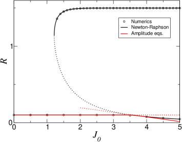
Figure 24: (Color online) Bifurcation diagram for the steady instability. Open circles: numerical simulation of Eq.(2). Red Lines: amplitude equation solution from Eq.(51). Black lines: steady-state solution of Eq.(2) using a Newton-Raphson solver. Solid lines indicate stable solutions and dotted lines unstable ones. $\Phi(x)=\frac{\alpha}{1+e^{-\beta x}}$ where $\alpha=1.5$ and $\beta=3$. $J(x)=J_{0}+J_{1}\cos{x}$ where $J_{1}=0$. The input current $I$ is varied so as to keep the uniform stationary solution fixed at $R=0.1$.

B.1.2 Turing bifurcation

$\vartheta(\epsilon)$: The solution to the linear equation is spatially periodic with slowly varying amplitude $A$,

$$r_{1}=A(T)e^{ix}+c.c.$$

$\vartheta(\epsilon^{2})$: The nonlinear forcing and resulting second order solution are

$$N_{2} = \Phi^{{}^{\prime\prime}}J_{1}^{2}(A^{2}e^{2ix}+c.c.+2|A|^{2})/2,$$

$$r_{2} = r_{22}e^{2ix}+c.c.+r_{20},$$

$$r_{22} = \frac{\Phi^{{}^{\prime\prime}}J_{1}^{2}}{2(1-J_{2}\Phi^{{}^{\prime}})}A^{2},$$

$$r_{20} = \frac{\Phi^{{}^{\prime\prime}}J_{1}^{2}}{1-J_{0}\Phi^{{}^{\prime}}}|A|^{2}.$$

$\vartheta(\epsilon^{3})$: The nonlinear forcing at cubic order is

$$N_{3}=(\Phi^{{}^{\prime\prime}}J_{1}J_{0}Ar_{20}+\Phi^{{}^{\prime\prime}}J_{1}J_{2}{A^{*}}r_{22}+\Phi^{{}^{\prime\prime\prime}}J_{1}^{3}|A|^{2}A/2)e^{ix}+c.c.+\dots$$

Eliminating all terms of periodicity $e^{ix}$ at this order yields the amplitude equation, Eq.(16).

$$\partial_{T}A=\eta\Delta J_{1}A+\Gamma|A|^{2}A,$$

with the coefficients

$$\eta = \frac{\Phi^{{}^{\prime}}}{1+D},$$

$$\Gamma = \frac{\bar{J}_{k}^{3}}{1+D}\Bigg{(}\frac{J_{0}(\Phi^{{}^{\prime\prime}})^{2}}{1-J_{0}\Phi^{{}^{\prime}}}+\frac{J_{2}(\Phi{{}^{\prime\prime}})^{2}}{2(1-J_{2}\Phi^{{}^{\prime}})}+\frac{\Phi^{{}^{\prime\prime\prime}}}{2}\Bigg{)}.$$

B.1.3 Hopf bifurcation

$\vartheta(\epsilon)$: The solution to the linear equation is a time periodic function with slowly varying amplitude $H$

$$r_{1}=H(T)e^{i\omega t}+c.c.$$

$\vartheta(\epsilon^{2})$: The nonlinear forcing and resulting second order solution are

$$N_{2} = \Phi^{{}^{\prime\prime}}J_{0}^{2}(H^{2}e^{2i\omega(t-D)}+c.c.+2|H|^{2})/2,$$

$$r_{2} = r_{22}e^{2i\omega t}+c.c.+r_{20},$$

$$r_{22} = \frac{\Phi^{{}^{\prime\prime}}J_{0}^{2}}{2(2i\omega+1-\Phi^{{}^{\prime}}J_{0}e^{-2i\omega D})}e^{-2i\omega D}H^{2},$$

$$r_{20} = \frac{\Phi^{{}^{\prime\prime}}J_{0}^{2}}{1-J_{0}\Phi^{{}^{\prime}}}|H|^{2}.$$

$\vartheta(\epsilon^{3})$: The nonlinear forcing at cubic order is

$$N_{3} = (\Phi^{{}^{\prime\prime}}J_{0}^{2}Hr_{20}+\Phi^{{}^{\prime\prime}}J_{0}^{2}{H^{*}}r_{22}$$

$$+ \Phi^{{}^{\prime\prime\prime}}J_{0}^{3}|A|^{2}A/2)e^{i\omega(t-D)}+c.c.+\dots$$

Eliminating all terms of periodicity $e^{i\omega t}$ at this order yields the amplitude equation, Eq.(18).

$$\partial_{T}H=(\mu+i\Omega)\Delta J_{0}H+(\alpha+i\beta)|H|^{2}H,$$

with the coefficients

$$\mu+i\Omega = \frac{\Phi^{{}^{\prime}}e^{-i\omega D}}{1+D(1+i\omega)},$$ (52)

$$\alpha+i\beta = \frac{e^{-i\omega D}}{1+D(1+i\omega)}\times$$

$$\Bigg{(}\frac{\bar{J}_{0}^{4}(\Phi^{{}^{\prime\prime}})^{2}}{1-\Phi^{{}^{\prime}}\bar{J}_{0}}+\frac{\bar{J}_{0}^{4}(\Phi^{{}^{\prime\prime}})^{2}e^{-2i\omega D}}{2(2i\omega+1-\Phi^{{}^{\prime}}\bar{J}_{0}e^{-2i\omega D})}+\frac{\bar{J}_{0}^{3}\Phi^{{}^{\prime\prime\prime}}}{2}\Bigg{)}.$$

B.1.4 Turing-Hopf bifurcation

$\vartheta(\epsilon)$: The solution to the linear equation are two sets of periodic waves, one left-traveling with slowly varying amplitude $A$ and the other right-traveling with slowly varying amplitude $B$

$$r_{1} = A(T)e^{i\omega t+ix}+B(T)e^{-i\omega t+ix}+c.c.$$

$$= A(T)e^{\psi}+B(T)e^{\phi}+c.c.$$

$\vartheta(\epsilon^{2})$: The nonlinear forcing and resulting second order solution are

$$N_{2} = \Phi^{{}^{\prime\prime}}J_{1}^{2}\Big{[}A^{2}e^{2\psi-2i\omega D}+2ABe^{\psi+\phi}+2A{B^{*}}e^{\psi+{\phi^{*}}-2i\omega D}+$$

$$B^{2}e^{2\phi+2i\omega D}+\text{c.c.}+2(|A|^{2}+|B|^{2})\Big{]}/2,$$

$$r_{2} = r_{2\psi}e^{2\psi}+r_{\psi\phi}e^{\psi+\phi}+r_{\psi{\phi^{*}}}e^{\psi+{\phi^{*}}}+r_{2\phi}e^{2\phi}+\text{c.c.}+r_{20},$$

$$r_{2\psi} = \frac{\Phi^{{}^{\prime\prime}}J_{1}^{2}}{2(2i\omega+1-\Phi^{{}^{\prime}}J_{2}e^{-2i\omega D})}e^{-2i\omega D}A^{2},$$

$$r_{\psi\phi} = \frac{\Phi^{{}^{\prime\prime}}J_{1}^{2}}{1-\Phi^{{}^{\prime}}J_{2}}AB,$$

$$r_{\psi{\phi^{*}}} = \frac{\Phi^{{}^{\prime\prime}}J_{1}^{2}}{2i\omega+1-J_{0}\Phi^{{}^{\prime}}e^{-2i\omega D}}e^{-2i\omega D}AB^{*},$$

$$r_{2\phi} = \frac{\Phi^{{}^{\prime\prime}}J_{1}^{2}}{2(-2i\omega D+1-J_{2}\Phi^{{}^{\prime}}e^{2i\omega D})}e^{2i\omega D}B^{2},$$

$$r_{20} = \frac{\Phi^{{}^{\prime\prime}}J_{1}^{2}(|A|^{2}+|B|^{2})}{1-J_{0}\Phi^{{}^{\prime}}}.$$

$\vartheta(\epsilon^{3})$: The nonlinear forcing at cubic order is

$$N_{3} = [\Phi^{{}^{\prime\prime}}J_{1}(J_{0}Ar_{20}+J_{2}{A^{*}}r_{2\psi}+J_{0}Br_{\psi{\phi^{*}}}+J_{2}{B^{*}}r_{\psi\phi})+$$

$$\Phi^{{}^{\prime\prime\prime}}(|A|^{2}A/2+|B|^{2}A)]e^{\psi-i\omega D}+$$

$$[\Phi^{{}^{\prime\prime}}J_{1}(J_{0}A{r^{*}}_{\psi{\phi^{*}}}+J_{2}{A^{*}}r_{\psi\phi}+J_{0}Br_{20}+J_{2}{B^{*}}r_{2\phi})+$$

$$\Phi^{{}^{\prime\prime\prime}}(|B|^{2}B/2+|A|^{2}B)]e^{\phi+i\omega D}+\dots$$

Eliminating all terms with dependencies $e^{i\psi}$ and $e^{i\phi}$ yields the two coupled amplitude equations (21a,21b):

$$\partial_{T}A = (\mu+i\Omega)\Delta J_{1}A+(a+ib)|A|^{2}A+(c+id)|B|^{2}A,$$

$$\partial_{T}B = (\mu-i\Omega)\Delta J_{1}B+(a-ib)|B|^{2}B+(c-id)|A|^{2}B,$$

with the coefficients

$$a+ib = \frac{\bar{J}_{k}^{3}e^{-i\omega D}}{1+D\Phi^{{}^{\prime}}\bar{J}_{k}e^{-i\omega D}}\times$$ (54)

$$\Bigg{(}\frac{J_{0}(\Phi^{{}^{\prime\prime}})^{2}}{1-\Phi^{{}^{\prime}}J_{0}}+\frac{J_{2}(\Phi^{{}^{\prime\prime}})^{2}e^{-2i\omega D}}{2(2i\omega+1-\Phi^{{}^{\prime}}J_{2}e^{-2i\omega D})}+\frac{\Phi^{{}^{\prime\prime\prime}}}{2}\Bigg{)},$$

$$c+id = \frac{\bar{J}_{k}^{3}e^{-i\omega D}}{1+D\Phi^{{}^{\prime}}\bar{J}_{k}e^{-i\omega D}}\times$$ (55)

$$\Bigg{(}\frac{J_{0}(\Phi^{{}^{\prime\prime}})^{2}}{1-\Phi^{{}^{\prime}}J_{0}}+\frac{J_{0}(\Phi^{{}^{\prime\prime}})^{2}e^{-2i\omega D}}{2i\omega+1-\Phi^{{}^{\prime}}J_{0}e^{-2i\omega D}}+\frac{J_{2}(\Phi^{{}^{\prime\prime}})^{2}}{1-\Phi^{{}^{\prime}}J_{2}}+\Phi^{{}^{\prime\prime\prime}}\Bigg{)}.$$

B.2 Codimension 2 bifurcations

B.2.1 Double zero eigenvalue: Hopf, Turing-Hopf

$\vartheta(\epsilon)$: The solution to the linear equation are periodic oscillations and traveling waves

$$r_{1}=H(T)e^{i\omega t}+A(T)e^{\psi}+B(T)e^{\phi}+c.c.$$

where we have defined $\psi\equiv i(kx+\omega t)$ and $\phi\equiv i(kx-\omega t)$.

$\vartheta(\epsilon^{2})$: The nonlinear forcing and resulting second order solution are

$$N_{2} = \Phi^{{}^{\prime\prime}}J_{0}^{2}(H^{2}e^{2i\omega(t-D)}+c.c.+2|H|^{2})/2+\Phi^{{}^{\prime\prime}}J_{1}^{2}[A^{2}e^{2\psi-2i\omega D}+2ABe^{\psi+\phi}$$

$$+2A{B^{*}}e^{\psi+{\phi^{*}}-2i\omega D}+B^{2}e^{2\phi+2i\omega D}+c.c.+2(|A|^{2}+|B|^{2})]/2$$

$$+\Phi^{{}^{\prime\prime}}J_{0}J_{1}(HAe^{2i\omega(t-D)+ix}+{H^{*}}Be^{-2i\omega(t-D)+ix}+A{H^{*}}e^{ix}+HBe^{ix}+c.c.),$$

$$r_{2} = r_{22}e^{2i\omega t}+r_{2\psi}e^{2\psi}+r_{\psi\phi}e^{\psi+\phi}+r_{\psi{\phi^{*}}}e^{\psi+{\phi^{*}}}+r_{2\phi}e^{2\phi}+r_{HA}e^{2i\omega t+ix}+$$

$$r_{B{H^{*}}}e^{-2i\omega t+ix}+r_{A{H^{*}}}e^{ix}+r_{HB}e^{ix}+c.c.+r_{20},$$

$$r_{HA} = \frac{\Phi^{{}^{\prime\prime}}J_{0}J_{1}}{2i\omega+1-\Phi^{{}^{\prime}}J_{1}e^{-2i\omega D}}e^{-2i\omega D}HA,$$

$$r_{B{H^{*}}} = \frac{\Phi^{{}^{\prime\prime}}J_{0}J_{1}}{-2i\omega+1-\Phi^{{}^{\prime}}J_{1}e^{2i\omega D}}e^{2i\omega D}B{H^{*}},$$

$$r_{A{H^{*}}} = \frac{\Phi^{{}^{\prime\prime}}J_{0}J_{1}}{1-\Phi^{{}^{\prime}}J_{1}}A{H^{*}},$$

$$r_{HB} = \frac{\Phi^{{}^{\prime\prime}}J_{0}J_{1}}{1-\Phi^{{}^{\prime}}J_{1}}HB,$$

$$r_{20} = \frac{\Phi^{{}^{\prime\prime}}(J_{0}^{2}|H|^{2}+J_{1}^{2}|A|^{2}+J_{1}^{2}|B|^{2})}{1-J_{0}\Phi^{{}^{\prime}}}.$$

$\vartheta(\epsilon^{3})$: The nonlinear forcing at cubic order is

$$N_{3} = [\Phi^{{}^{\prime\prime}}J_{0}^{2}(Hr_{20}+{H^{*}}r_{22})+\Phi^{{}^{\prime\prime}}J_{1}^{2}(A{r^{*}}_{A{H^{*}}}+{A^{*}}r_{HA}+{B^{*}}r_{A{H^{*}}}+$$

$$B{r^{*}}_{B{H^{*}}}+A{r^{*}}_{HB}+{B^{*}}r_{HB})+\Phi^{{}^{\prime\prime\prime}}J_{0}^{3}|H|^{2}H/2]e^{i\omega(t-D)}+$$

$$[\Phi^{{}^{\prime\prime}}J_{1}(J_{0}Ar_{20}+J_{2}{A^{*}}r_{2\psi}+J_{0}Br_{\psi{\phi^{*}}}+J_{2}{B^{*}}r_{\psi\phi}+$$

$$J_{0}(Hr_{A{H^{*}}}+Hr_{HB}+{H^{*}}r_{HA}))+\Phi^{{}^{\prime\prime\prime}}(|A|^{2}A/2+|B|^{2}A)]e^{\psi-i\omega D}+$$

$$[\Phi^{{}^{\prime\prime}}J_{1}(J_{0}A{r^{*}}_{\psi{\phi^{*}}}+J_{2}{A^{*}}r_{\psi\phi}+J_{0}Br_{20}+J_{2}{B^{*}}r_{2\phi}]+$$

$$J_{0}(Hr_{B{H^{*}}}+{H^{*}}r_{A{H^{*}}}+{H^{*}}r_{HB}))+\Phi^{{}^{\prime\prime\prime}}(|B|^{2}B/2+|A|^{2}B)]e^{\phi+i\omega D}+\dots$$

Eliminating terms with dependencies $e^{i\omega t}$, $e^{i\psi}$ and $e^{i\phi}$ yields the three coupled amplitude equations (27-27c):

$$\partial_{T}H = (\mu+i\Omega)\Delta J_{0}H+2(\alpha+i\beta)\Big{[}(\frac{|H|^{2}}{2}+|A|^{2}+|B|^{2})H+A{H^{*}}{B^{*}}\Big{]},$$

$$\partial_{T}A = (\mu+i\Omega)\Delta J_{1}A+(a+ib)|A|^{2}A+(c+id)|B|^{2}A+$$

$$(\alpha+i\beta)(2|H|^{2}A+H^{2}B),$$

$$\partial_{T}B = (\mu-i\Omega)\Delta J_{1}B+(a-ib)|B|^{2}B+(c-id)|A|^{2}B+$$

$$(\alpha-i\beta)(2|H|^{2}B+{H^{*}}^{2}A),$$

where $\alpha+i\beta$, $a+ib$ and $c+id$ are given by Eqs. (B.1.3, 54,55), respectively.

In the small delay limit ($D\to 0$) we can use the asymptotic values given by Eqs. (11) to obtain, to leading order,

$$a+ib = -\frac{\chi(\frac{\pi}{2}+i)}{(D\Phi)^{3}}\Bigg{(}\frac{(\Phi^{{}^{\prime\prime}})^{2}}{\Phi^{{}^{\prime}}}-\frac{\Phi^{{}^{\prime\prime\prime}}}{2}\Bigg{)},$$ (56)

$$c+id = -\frac{\chi}{(D\Phi)^{3}}\Bigg{(}\frac{(\Phi^{{}^{\prime\prime}})^{2}}{\Phi^{{}^{\prime}}}\frac{(3\pi-2)}{5}-\frac{\pi}{2}\frac{J_{2}(\Phi^{{}^{\prime\prime}})^{2}}{1-\Phi^{{}^{\prime}}J_{2}}-\frac{\pi\Phi^{{}^{\prime\prime\prime}}}{2}+$$ (57)

$$i\Bigg{[}\frac{(\Phi^{{}^{\prime\prime}})^{2}}{\Phi^{{}^{\prime}}}\frac{(6+\pi)}{5}-\frac{J_{2}(\Phi^{{}^{\prime\prime}})^{2}}{1-\Phi^{{}^{\prime}}J_{2}}-\Phi^{{}^{\prime\prime\prime}}\Bigg{]}\Bigg{)}.$$

where $\chi\equiv\pi^{3}/(8+2\pi^{2})$ and $\alpha+i\beta$ is given by Eq.(19b).

Figure 25: Top: The real part of the cubic coefficient at the codimension-2 point. The solid line is the full expression, Eq.(54) and the dotted line is the asymptotic result in the $D\to 0$ limit, Eq.(56). Bottom: The real part of the cross-coupling coefficient at the codimension-2 point. The solid line in the full expression, Eq.(55) and the dotted line is the asymptotic results in the $D\to 0$ limit, Eq.(57).

Solutions and their stability

Oscillatory uniform OU:

This solution can be expressed as $(H,A,B)=(\mathcal{H}e^{i\omega t},0,0)$, where

$$\mathcal{H} = \sqrt{\frac{-\mu\Delta J_{0}}{\alpha}},$$

$$\omega = \Big{(}\Omega-\frac{\beta\mu}{\alpha}\Big{)}\Delta J_{0}.$$

The stability of this solution can be studied with the ansatz

$$(H,A,B) = (M\mathcal{H}e^{i\omega t}(1+\delta H_{+}e^{\lambda t}+{\delta H^{*}}_{-}e^{{\lambda^{*}}t}),e^{i\omega t}(\delta A_{+}e^{\lambda t}+{\delta A^{*}}_{-}e^{{\lambda^{*}}t}),$$

$$e^{-i\omega t}(\delta B_{+}e^{\lambda t}+{\delta B^{*}}_{-}e^{{\lambda^{*}}t})),$$

which leads to three pairs of coupled linear equations which determine the six eigenvalues $\lambda$. The first pair is restricted to the linear subspace of the small amplitude limit cycle and results in the standard stability problem which yields one stable eigenvalue $\lambda=-\mu\Delta J_{0}$ and one zero eigenvalue corresponding to a shift in the phase of the oscillation. The other two pairs, which span the subspaces of $(\delta A_{+},\delta B_{+})$ and $(\delta A_{-},\delta B_{-})$ respectively, give

$$\left(\begin{array}[]{cc}M&-(\alpha+i\beta)\mathcal{H}^{2}\\ -(\alpha-i\beta)\mathcal{H}^{2}&M^{*}\end{array}\right)\left(\begin{array}[]{c}\delta A_{+}\\ \delta B_{+}\end{array}\right)=0,$$ (61)

where $M=\lambda-\mu\Delta J_{1}-2\alpha\mathcal{H}^{2}+i(\Omega(\Delta J_{0}-\Delta J_{1})-\beta\mathcal{H}^{2})$, and the complex conjugate matrix spanning $(\delta A_{-},\delta B_{-})$. Setting the determinant equal to zero yields the characteristic equation

$$0 = \lambda^{2}-2\lambda(\Delta J_{1}-2\Delta J_{0})\mu+\mu^{2}(\Delta J_{1}-4\Delta J_{1}\Delta J_{0}+3\Delta J_{0})+$$

$$\Omega^{2}(\Delta J_{1}-\Delta J_{0})^{2}-2\frac{\beta}{\alpha}\mu\Omega\Delta J_{0}(\Delta J_{1}-\Delta J_{0}).$$

We find an oscillatory instability for $\Delta J_{1}=2\Delta J_{2}$ while a steady instability occurs for $\Delta J_{1}=\Delta J_{0}$. The steady instability therefore always precedes the oscillatory one.

Traveling waves (TW):

This solution can be expressed as $(H,A,B)=(0,\mathcal{A}_{TW}e^{i\omega t},0)$, where

$$\mathcal{A}_{TW} = \sqrt{\frac{-\mu\Delta J_{1}}{a}},$$

$$\omega = \Big{(}\Omega-\frac{b\mu}{a}\Big{)}\Delta J_{1}.$$

The stability of this solution can be studied with the ansatz

$$(H,A,B) = (e^{i\omega t}(\delta H_{+}e^{\lambda t}+{\delta H^{*}}_{-}e^{{\lambda^{*}}t}),\mathcal{A}_{TW}e^{i\omega t}(1+\delta A_{+}e^{\lambda t}+{\delta A^{*}}_{-}e^{{\lambda^{*}}t}),$$

$$e^{-i\omega t}(\delta B_{+}e^{\lambda t}+{\delta B^{*}}_{-}e^{{\lambda^{*}}t})),$$

which results in four coupled linear equations corresponding to the stability problem for TW in the competition between SW and TW (see section D, Turing-Hopf Bifurcation). Here we assume that the TW solution is supercritical and stable. We then turn our attention to the remaining two linear equations which describe the growth of the oscillatory uniform mode. These equations are uncoupled and yield the complex conjugate eigenvalues

$$\lambda=-\mu\Big{(}2\frac{\alpha}{a}\Delta J_{1}-\Delta J_{0}\Big{)}\pm i\Big{(}\Omega(1-\frac{a}{2\alpha})+(b-2\beta)\frac{\mu}{2\alpha}\Big{)}\Delta J_{0},$$

from which it is easy to see that an instability occurs for $\Delta J_{1}=\frac{a}{2\alpha}\Delta J_{0}$. This instability will generically occur with non-zero frequency.

Standing waves (SW):

This solution can be expressed as $(H,A,B)=(0,\mathcal{A}_{SW}e^{i\omega t},\mathcal{A}_{SW}e^{-i\omega t})$, where $\mathcal{A}_{SW}$ and $\omega$ are given by Eqs. (30, 31)

$$\mathcal{A}_{SW} = \sqrt{\frac{-\mu\Delta J_{1}}{(a+c)}},$$

$$\omega = \Big{(}\Omega-\frac{(b+d)}{(a+c)}\mu\Big{)}\Delta J_{1}.$$

The stability of this solution can be studied with the ansatz

$$(H,A,B) = (e^{i\omega t}(\delta H_{+}e^{\lambda t}+{\delta H^{*}}_{-}e^{{\lambda^{*}}t}),\mathcal{A}_{SW}e^{i\omega t}(1+\delta A_{+}e^{\lambda t}+{\delta A^{*}}_{-}e^{{\lambda^{*}}t}),$$

$$\mathcal{A}_{SW}e^{-i\omega t}(1+\delta B_{+}e^{\lambda t}+{\delta B^{*}}_{-}e^{{\lambda^{*}}t})).$$

This ansatz results in four coupled equations for the stability of SW in the competition between SW and TW. Here we assume that the SW solution is supercritical and stable. The remaining two equations describe the growth of the oscillatory uniform mode.

$$\left(\begin{array}[]{cc}N&-2\mathcal{A}_{SW}(\alpha+i\beta)\\ -2\mathcal{A}_{SW}(\alpha-i\beta)&N^{*}\end{array}\right)\left(\begin{array}[]{c}\delta H_{+}\\ \delta H_{-}\end{array}\right)=0.$$ (66)

where $N=\lambda+i\omega-(\mu+i\Omega)\Delta J_{0}-4\mathcal{A}_{SW}(\alpha+i\beta)$. Setting the determinant to zero yields the characteristic equation for the eigenvalues

$$0 = \mu^{2}\left(\Delta J_{0}-\frac{4\alpha\Delta J_{1}}{(a+c)}\right)^{2}+\Big{(}\Delta J_{1}\Big{[}\Omega-\frac{(b+d)\mu}{(a+c)}+\frac{4\beta\mu}{(a+c)}\Big{]}-\Omega\Delta J_{0}\Big{)}^{2}-$$ (67)

$$\frac{4\mu^{2}\Delta J_{1}^{2}(\alpha^{2}+\beta^{2})}{(a+c)^{2}}-2\mu\lambda\Big{[}\Delta J_{0}-\frac{4\alpha\Delta J_{1}}{(a+c)}\Big{]}+\lambda^{2}.$$

The conditions for oscillatory and steady instabilities  (32,33), are found by setting $\lambda$ equal to $i\bar{\omega}$ and $0$ respectively.

Mixed Mode:

Mixed mode solutions are found by applying the ansatz Eq.(35) to Eqs. (27-27c). This gives

$$\dot{\mathcal{H}} = \mu\Delta J_{0}\mathcal{H}+\alpha(\mathcal{H}^{2}+2\mathcal{A}^{2}+2\mathcal{B}^{2})\mathcal{H}+2\mathcal{HAB}(\alpha\cos{\phi}-\beta\sin{\phi}),$$

$$\dot{\mathcal{A}} = \mu\Delta J_{1}\mathcal{A}+a\mathcal{A}^{3}+c\mathcal{B}^{2}\mathcal{A}+2\alpha\mathcal{H}^{2}\mathcal{A}+\mathcal{H}^{2}\mathcal{B}(\alpha\cos{\phi}+\beta\sin{\phi}),$$

$$\dot{\mathcal{B}} = \mu\Delta J_{1}\mathcal{B}+a\mathcal{B}^{3}+c\mathcal{A}^{2}\mathcal{B}+2\alpha\mathcal{H}^{2}\mathcal{B}+\mathcal{H}^{2}\mathcal{A}(\alpha\cos{\phi}+\beta\sin{\phi}),$$

$$\dot{\phi} = 2\Omega(\Delta J_{1}-\Delta J_{0})+2\beta\mathcal{H}^{2}+(b+d-4\beta)(\mathcal{A}^{2}+\mathcal{B}^{2})-$$ (68)

$$\alpha\sin{\phi}\Big{(}\frac{\mathcal{H}^{2}\mathcal{B}}{\mathcal{A}}+\frac{\mathcal{H}^{2}\mathcal{A}}{\mathcal{B}}+4\mathcal{AB}\Big{)}+\beta\cos{\phi}\Big{(}\frac{\mathcal{H}^{2}\mathcal{B}}{\mathcal{A}}+\frac{\mathcal{H}^{2}\mathcal{A}}{\mathcal{B}}-4\mathcal{AB}\Big{)},$$

where $\phi=\psi_{A}-\psi_{B}-2\theta$. One steady state solution of these equations takes the form $(\mathcal{H},\mathcal{A},\mathcal{B},\phi)=(\mathcal{\hat{H}},\mathcal{\hat{A}},-\mathcal{\hat{A}},\hat{\phi})$, where

$$\mathcal{\hat{H}}^{2} = \frac{-\mu\Delta J_{0}(a+c)-2\mu\Delta J_{1}\big{(}-2\alpha+\alpha\cos{\hat{\phi}}-\beta\sin{\hat{\phi}}\big{)}}{\alpha(a+c)-\big{[}4\alpha-2(\alpha\cos{\hat{\phi}}-\beta\sin{\hat{\phi}})\big{]}\big{[}2\alpha-\alpha\cos{\hat{\phi}}+\beta\sin{\hat{\phi}}\big{]}},$$ (69)

$$\mathcal{\hat{A}}^{2} = \frac{-\mu\Delta J_{0}(-2\alpha+\alpha\cos{\hat{\phi}}-\beta\sin{\hat{\phi}})-\mu\Delta J_{1}\alpha}{\alpha(a+c)-\big{[}4\alpha-2(\alpha\cos{\hat{\phi}}-\beta\sin{\hat{\phi}})\big{]}\big{[}2\alpha-\alpha\cos{\hat{\phi}}+\beta\sin{\hat{\phi}}\big{]}},$$ (70)

and $\hat{\phi}$ is found by plugging Eqs. (69,70) into Eq.(68) and setting the left hand side equal to zero. We do not study the stability of the mixed-mode state here.

B.2.2 Double zero eigenvalue: Turing, Hopf

$\vartheta(\epsilon)$: The solutions to the linear equation are time periodic oscillations and spatially periodic functions

$$r_{1}=H(T)e^{i\omega t}+A(T)e^{ix}+c.c.$$

$\vartheta(\epsilon^{2})$: The nonlinear forcing and resulting second order solution are

$$N_{2} = \frac{\Phi^{{}^{\prime\prime}}}{2}J_{0}^{2}(H^{2}e^{2i\omega(t-D)}+c.c.+2|H|^{2})+\frac{\Phi^{{}^{\prime\prime}}}{2}J_{1}^{2}(A^{2}e^{2ix}+c.c.+2|A|^{2})$$

$$\Phi^{{}^{\prime\prime}}J_{0}J_{1}HAe^{ix+i\omega t}+\Phi^{{}^{\prime\prime}}J_{0}J_{1}A{H^{*}}e^{-i\omega t+ix}+c.c.,$$

$$r_{2} = r_{2H}e^{2i\omega t}+r_{2A}e^{2ix}+r_{AH}e^{i\omega t+ix}+r_{A{H^{*}}}e^{-i\omega t+ix}+c.c.+r_{20},$$

$$r_{AH} = \frac{\Phi^{{}^{\prime\prime}}J_{0}J_{1}}{i\omega+1-\Phi^{{}^{\prime}}J_{1}e^{-i\omega D})}e^{-i\omega D}AH,$$

$$r_{A{H^{*}}} = \frac{\Phi^{{}^{\prime\prime}}J_{0}J_{1}}{-i\omega+1-\Phi^{{}^{\prime}}J_{1}e^{i\omega D}}e^{i\omega D}A{H^{*}},$$

$$r_{20} = \frac{\Phi^{{}^{\prime\prime}}(J_{0}^{2}|H|^{2}+J_{1}^{2}|A|^{2})}{1-J_{0}\Phi^{{}^{\prime}}}.$$

$\vartheta(\epsilon^{3})$: The nonlinear forcing at cubic order is

$$N_{3} = \Big{[}\Phi^{{}^{\prime\prime}}(J_{0}^{2}Hr_{20}+J_{0}^{2}{H^{*}}r_{2H}+J_{1}^{2}A{r^{*}}_{A\hat{H}}+J_{1}^{2}{A^{*}}r_{AH})+$$

$$\Phi^{{}^{\prime\prime\prime}}(J_{0}^{2}J_{1}|H|^{2}A+J_{1}^{3}|A|^{2}A/2)\Big{]}e^{i\omega t}+$$

$$\Big{[}\Phi^{{}^{\prime\prime}}(J_{0}J_{1}Hr_{A{H^{*}}}+J_{0}J_{1}{H^{*}}r_{AH}+J_{0}J_{1}Ar_{20}+J_{1}J_{2}{A^{*}}r_{2A})+$$

$$\Phi^{{}^{\prime\prime\prime}}(J_{0}^{2}J_{1}|H|^{2}A+J_{1}^{3}|A|^{2}A/2)\Big{]}e^{ix}.$$

Eliminating terms with dependencies $e^{i\omega t}$, $e^{ix}$ yields the two coupled amplitude equations, Eqs. (38a-38b),

$$\partial_{T}H = (\mu+i\Omega)\Delta J_{0}H+(\alpha+i\beta)|H|^{2}H+(\kappa+i\Lambda)|A|^{2}H,$$

$$\partial_{T}A = \bar{\eta}\Delta J_{1}A+\Gamma|A|^{2}A+\sigma|H|^{2}A,$$

where $\mu+i\Omega$, $\alpha+i\beta$, $\bar{\eta}$ and $\Gamma$ are given by Eqs. (52, B.1.3,17a, 17b) respectively, and

$$\kappa+i\Lambda = \frac{e^{-i\omega D}}{1+D\Phi^{{}^{\prime}}\bar{J}_{0}e^{-i\omega D}}\Bigg{(}\frac{\bar{J}_{0}^{2}\bar{J}_{k}^{2}}{1-\Phi^{{}^{\prime}}\bar{J}_{0}}+2\frac{\bar{J}_{1}^{3}\bar{J}_{0}(\Phi^{{}^{\prime\prime}})^{2}e^{-i\omega D}}{i\omega+1-\Phi^{{}^{\prime}}\bar{J}_{1}e^{-i\omega D}}+$$ (71)

$$\Phi^{{}^{\prime\prime\prime}}\bar{J}_{0}\bar{J}_{1}^{2}\Bigg{)},$$

$$\sigma = \frac{1}{1+D\Phi^{{}^{\prime}}\bar{J}_{1}}\Bigg{(}\frac{\bar{J}_{0}^{3}\bar{J}_{1}(\Phi^{{}^{\prime\prime}})^{2}}{1-\Phi^{{}^{\prime}}\bar{J}_{0}}+\Phi^{{}^{\prime\prime\prime}}\bar{J}_{0}^{2}\bar{J}_{1}+\bar{J}_{0}^{2}\bar{J}_{1}^{2}(\Phi^{{}^{\prime\prime}})^{2}\times$$ (72)

$$\Big{(}\frac{e^{i\omega D}}{-i\omega+1-\Phi^{{}^{\prime}}\bar{J}_{1}e^{i\omega D}}+\frac{e^{-i\omega D}}{i\omega+1-\Phi^{{}^{\prime}}\bar{J}_{1}e^{-i\omega D}}\Big{)}\Bigg{)}.$$

In the small delay limit ($D\to 0$) we can use the asymptotic values (11) to obtain, to leading order,

$$\kappa+i\Lambda = -\frac{\pi}{2D(\Phi^{{}^{\prime}})^{3}}\frac{(\pi/2+i)}{(1+\pi^{2}/4)}\Bigg{(}\frac{(\Phi^{{}^{\prime\prime}})^{2}}{\Phi^{{}^{\prime}}}-\Phi^{{}^{\prime\prime\prime}}\Bigg{)}+\vartheta(1),$$

$$\eta = \Phi^{{}^{\prime}}+\vartheta(D),$$

$$\Gamma = \frac{1}{(\Phi^{{}^{\prime}})^{3}}\Bigg{(}-\frac{(\Phi^{{}^{\prime\prime}})^{2}}{\Phi^{{}^{\prime}}}+\frac{\Phi^{{}^{\prime\prime\prime}}}{2}+\frac{J_{2}(\Phi^{{}^{\prime\prime}})}{2(1-J_{2}\Phi^{{}^{\prime}})}\Bigg{)}+\vartheta(D),$$

$$\sigma = -\frac{\pi^{2}}{4D^{2}(\Phi^{{}^{\prime}})^{3}}\Bigg{(}\frac{(\Phi^{{}^{\prime\prime}})^{2}}{\Phi^{{}^{\prime}}}-\Phi^{{}^{\prime\prime\prime}}\Bigg{)}+\vartheta(1/D),$$

and $\mu+i\Omega$ and $\alpha+i\beta$ are given by Eqs. (19a,19b) respectively.

References

- [1] A. Roxin, N. Brunel and D. Hansel, Phys. Rev. Lett 94, 238103 (2005).
- [2] A. Roxin, N. Brunel, D. Hansel, Prog. Theor. Phys. 161, 68 (2006).
- [3] N. Brunel, and V. Hakim, Neural Comp. 11, 1621 (1999).
- [4] N. Brunel, J. Comput. Neurosci. 8, 183 (2000).
- [5] D. J. Amit, and N. Brunel, Cerebral Cortex 7, 237 (1997).
- [6] G. B. Ermentrout, Rep. Prog. Phys. 61, 353 (1998).
- [7] S. Coombes, Biol. Cybern. 93, 91 (2005).
- [8] H. R. Wilson, and J. D. Cowan, Biophys. J. 12, 1 (1972).
- [9] S. Amari, Biol. Cybern. 27, 77 (1977).
- [10] G. B. Ermentrout, Neural Comp. 6, 679 (1994).
- [11] O. Shriki, D. Hansel, and H. Sompolinsky, Neural Comput. 15 1809-1841 (2003)
- [12] G. B. Ermentrout, and J. B. McLeod, Proc. R. Soc. Edin. 123A, 461 (1993).
- [13] D. J. Pinto, and G. B. Ermentrout, SIAM J. Appl. Math. 62, 206 (2001).
- [14] D. J. Pinto, and G. B. Ermentrout, SIAM J. Appl. Math. 62, 226 (2001).
- [15] C. Holmgren, T. Harkany, B. Svennenfors, and Y. Zilberter, J. Physiol. 551, 139 (2003).
- [16] A. Hutt, M. Bestehorn, and T. Wennekers, Network 14, 351 (2003).
- [17] S. Coombes, G. J. Lord and M. R. Owen, Physica D 178, 219 (2003).
- [18] A. Hutt, Phys Rev. E 70, 052902 (2004).
- [19] A. Hutt, and F. M. Atay, Phys. Rev. E 73, 021906 (2006).
- [20] F. M. Atay, and A. Hutt, SIAM J. Appl. Math. 65, 644 (2005).
- [21] V. K. Jirsa, and H. Haken, Phys. Rev. Lett. 77, 960 (1996)
- [22] N. A. Venkov, S. Coombes, and P. C. Matthews, Physica D 232, 1 (2007).
- [23] C. R. Laing, and S. Coombes, Network 17, 151 (2005).
- [24] S. Coombes, N. A. Venkov, L. Shiau, I. Bojak, D. T. J. Liley, and C. R. Laing, Phys. Rev. E 76, 051901 (2007).
- [25] M. C. Cross, and P. C. Hohenberg, Rev. Mod. Phys. 65, 851 (1993).
- [26] F. M. Atay, and A. Hutt, SIAM J. Appl. Dyn. Syst. 5, 670 (2006).
- [27] A. Hutt, C. Sutherland, and A. Longtin, Phys. Rev. E 78, 021911 (2008).
- [28] J. A. Roberts, and P. A. Robinson, Phys. Rev. E 78, 051901 (2008).
- [29] D. Battaglia, N. Brunel, and D. Hansel, Phys. Rev. Lett. 99, 238106 (2007)
- [30] S. Coombes, and C. Laing, Philos. Trans. R. Soc. A 367, 1117 (2009).
- [31] R. Ben-Yishai, R. Lev Bar-Or, and H. Sompolinsky, Proc. Natl. Acad. Sci. USA 92, 3844 (1995).
- [32] D. Hansel, and H. Sompolinsky, inMethods in Neuronal Modeling, edited by C. Koch and I. Segev (MIT press, Cambridge, MA, 1998), 2nd ed.
- [33] R. Curtu and B. Ermentrout, SIAM J. Applied Dynamical Systems. 3, 191 (2004).
- [34] N. Brunel and X. J. Wang, J. Neurophysiol. 90, 415 (2003).
- [35] C. Geisler, N. Brunel and X. J. Wang, J. Neurophysiol. 94, 4344 (2005).
- [36] D. Hansel, and C. van Vreeswijk, J. Neurosci. 22, 5118 (2002).
- [37] A. M. Thomson, and C. Lamy, Fontiers in Neuroscience 1, 19 (2007).
- [38] E. Kandel, J. H. Schwartz, and T. M. Jessell, Principles of Neural Science (Mc.Graw Hill, 1991).
- [39] P. Girard, J. M. Hupé, and J. Bullier, J. Neurophysiol. 85,1328 (2001).
- [40] G. B. Ermentrout, and J. D. Cowan, SIAM J. on Appl. Math. 38, 1 (1980).
- [41] E. K. Miller, and T. W. Troyer, J. Neurophysiol. 87, 653 (2002).
- [42] B. Hellwig, Biol. Cyber. 82, 111 (2000).
- [43] X.-J. Wang, and G. Buzsáki, J. Neurosci. 16, 6402 (1996).
- [44] M. H. Holmes, Introduction to Perturbation Methods (Springer, New York, 1995).