Perturbation propagation in random and evolved Boolean networks

Abstract

We investigate the propagation of perturbations in Boolean networks by evaluating the Derrida plot and modifications of it. We show that even small Random Boolean Networks agree well with the predictions of the annealed approximation, but non-random networks show a very different behaviour. We focus on networks that were evolved for high dynamical robustness. The most important conclusion is that the simple distinction between frozen, critical and chaotic networks is no longer useful, since such evolved networks can display properties of all three types of networks. Furthermore, we evaluate a simplified empirical network and show how its specific state space properties are reflected in the modified Derrida plots.

I Introduction

Boolean networks (BNs) are used to model the dynamics of a wide variety of complex systems, ranging from neural networks rosen-zvi and social systems moreira04 to gene regulation networks lagomarsino , sometimes combined with evolutionary processes bassler04 ; agnespaper . BNs are composed of interacting nodes with binary states, typically $0$ and $1$, coupled among each other. The state of each node evolves according to a function of the states observed in a certain neighbourhood, similar to what is done when using cellular automata herrmann88 , but in contrast to cellular automata, BNs have no regular lattice structure, and not all nodes are assigned the same update function.

An often studied class of BNs are Random BNs (RBNs). In such networks, connections between nodes and functions are assigned at random. The dynamics of RBNs can be classified into frozen, chaotic and critical derrida . In a frozen network, a perturbation at one node propagates in one time step on an average to less than one other node. Starting from a random initial state, such networks freeze after a short time completely (apart from possibly a small number of nonfrozen nodes). Therefore attractors of the dynamics have typically length 1 (i.e., they are fixed points) or are very short. In a chaotic network, a perturbation at one node propagates in one time step on an average to more than one other node. The attractors of the dynamics are long, and a nonvanishing proportion of all nodes remains nonfrozen. Critical networks are at the boundary between these two phases, a perturbation at one node propagates in one time step on an average to exactly one other node.

Whether a RBN is frozen, critical or chaotic, can be determined by using the annealed approximation, which is a mean-field theory. It neglects correlations between nodes or states of nodes and corresponds to a system where the connections are newly assigned at each time step. Furthermore, since the annealed approximation neglects fluctuations, it applies to the limit of infinite network size. Usually, the phase diagram derived analytically by using the annealed approximation is correct for RBNs.

RBNs were originally introduced by S. Kauffman as a simple model for gene regulation networks kauffman:metabolic . Since he considered frozen and chaotic networks as biologically unrealistic, he suggested that biological networks are in a critical state “at the edge of chaos”. Although it has been shown in the meantime that critical RBNs have unrealistically large mean attractor numbers and attractor lengths samuelssontroein ; ourscalingpaper , the idea that cellular networks may be poised at a critical state is still alive. The concept of phase transitions, borrowed from equilibrium statistical physics, is thus carried over to biological systems, which are far from equilibrium.

In this paper, we address the question whether the simple classification of the dynamics of networks into frozen, chaotic and critical is still appropriate when networks are not assembled randomly. In fact, it was found that networks that were generated by some evolutionary algorithm, may have a very long but unique attractor that attracts all of state space sevim , or that in such networks initially similar states may diverge at first exponentially fast but then converge to the same fixed point agnespaper . These are two examples where features of the “frozen” and “chaotic” phases are united within the same network.

In order to better understand when and how some networks can combine features of different phases, we investigate the so-called Derrida plot derrida . The Derrida plot maps the initial Hamming distance between the states of two identical networks (the number of nodes with differing states) onto that obtained after one time step. We will show in the next section that for RBNs the properties of the Derrida plot and modifications derived from it agree with the predictions of the annealed approximation and with the simple classification into frozen, critical and chaotic networks. In section III, we focus on networks that were evolved for high dynamical robustness. We will see that the annealed approximation cannot be applied consistently to such networks, and that features of different “phases” are visible in the Derrida plot and related graphs. In section IV, we evaluate the Derrida plot and its modifications for a model of the yeast cell cycle network Li , which shows again deviations from the annealed approximation.

II RBNs

II.1 The Derrida plot

We consider RBNs of $N$ nodes with a fixed number $K$ of randomly assigned inputs per node and with the update function at each node chosen at random among all possible update functions. Such networks are frozen for $K<2$, critical for $K=2$, and chaotic for $K>2$ annealed .

In order to evaluate the Derrida plot, two copies of the same network are initialized in the same random initial state. Then the state of $h$ nodes of one copy are inverted. The Hamming distance between the two copies is now $h$. Then, both networks are updated once (i.e., one time step is considered), and the Hamming distance is evaluated again. For a given network, this procedure is repeated several times for each value of $h$ from 0 to $N$, and the average is taken for each value $h$.

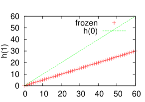
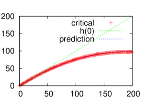
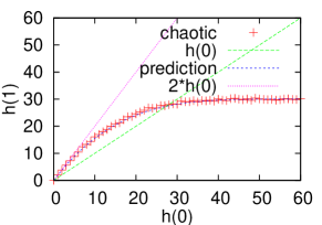
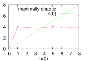
Figure 1: Derrida plot of RBNs with $K=1$, $N=60$; $K=2$, $N=200$; $K=4$, $N=60$; and $K=N=8$. The lines connecting the symbols are only guides to the eye.

The resulting Derrida plots are shown in figure 1 for a frozen ($K=1$, $N=60$), a critical ($K=2$, $N=200$), a chaotic ($K=4$, $N=60$) and a maximally chaotic ($K=N$ for $N=8$) network. Each point in the four plots is the average over at least 200 different perturbations and initial conditions.

The Derrida plot has the following properties, which can be easily explained within the annealed approximation annealed ; Kesseli :

1. In the frozen phase ($K=1$), the Derrida plot is linear and has the slope 1/2. In networks with $K=1$, there are 4 possible update functions, two of which are constant functions, the other two being the “copy” function and the “invert” function. These are assigned to the nodes with equal probability, which means that half of the nodes have a constant function and are therefore at time $t=1$ certainly in the same state in the two copies. The probability that a given node is not in the same state in the two copies at time $t=1$ is therefore 0.5 times the probability $h/N$ that the state of its input node differs at time $t=0$ in the two copies.

2. For $K=2$, the initial slope of the Derrida plot has the critical value 1. The probability that the state of a given node is different in the two copies at time $t=1$ is

   $$\frac{h(1)}{N}=r(1-(1-h(0)/N)^{K})\,,$$ (1)

   which is the probability that the state of at least one of its inputs is different in the two copies, times the probability $r$ that a difference in one or more inputs leads to a difference in the output. The slope of the function $h(1)$ vs $h(0)$ is $rK$ for small $h(0)$. When using all update functions with the same probability (as we have done), $r$ is equal to $1/2$.

3. In the chaotic phase, with fixed $K$, and with $N\gg K$, the initial slope of the Derrida plot is $Kr=K/2$. The probability that the state of a given node is different in the two copies at time $t=1$ is again given by equation (1) with $r=1/2$.

4. For RBNs with $K=N$, the average distance between any two non-identical states is $N/2$ after one time step, because each node changes its state with probability $r=1/2$, since the inputs differ in at least one node derACKreview .

Although the simulated networks are relatively small, their Derrida plot agrees very well with the one predicted by the annealed approximation. The relation between $h(1)$ and $h(0)$ derived from equation (1) matches perfectly the results of the simulations for the critical and the chaotic network, so that it is hard to distinguish the two lines in figure 1.

In order to prepare the discussion in section III, it is useful to consider also other graphs related to the Derrida plot, which will then be used to compare random and evolved networks.

II.2 The generalized Derrida plot

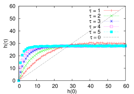
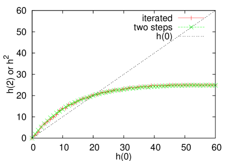
Figure 2: Generalized Derrida plot of a network with $K=4$, $N=60$, for different numbers of iterations $\tau$.

Figure 3: Generalized Derrida plot $h(2)$ (“two steps”, x symbols) and iterated Derrida map $h^{2}$ (“iterated”, + symbols) of a network with $K=3$, $N=60$.

First, we generated generalized Derrida plots by evaluating the Hamming distance $h(t>1)$ after more than one iteration as function of $h(0)$. We will compare the generalized Derrida plot with the iterated Derrida map. If we denote the Derrida map by $h(1)=f(h(0))$, the iterated map is $f(f(h(0)))$ for two iterations, and correspondingly for higher iterations. In the following, we will denote the twice iterated map $f(f(h(0)))$ simply by $h^{2}$.

Figure 3 shows $h(t)$ as function of $h(0)$ for $t=1,...,5$ for the above chaotic network with $K=4$. Each data point in this and in the following figures is averaged over 1000 randomly chosen combinations of the initial state and the perturbed nodes. The lines connecting the points are only guides to the eye. Within the annealed approximation, we expect $h(2)=h^{2}$, and equivalently for larger times. This is because the annealed approximation neglects correlations between nodes or between different times, and therefore the Hamming distance at one moment in time depends only on the Hamming distance in the previous time step, but not on the precise state of the system. If the annealed approximation is valid for the generalized Derrida plot for the RBN, not only the relation $h(2)=h^{2}$ must be satisfied, but also all plots for $h(t>1)$ must have the same fixed points, i.e. they must intersect the bisector at the same points. Figures 3 and 3 show that these two conditions are indeed satisfied. For critical and frozen networks, we found the same quality of agreement. Further below, we will see that no such agreement can be seen for evolved networks.

Such a good agreement between the annealed approximation and the simulation data is even more surprising considering the fact that the sizes of the networks are relatively small. The annealed approximation can be expected to become exact in the thermodynamic limit of infinite system size.

II.3 The modified Derrida plot

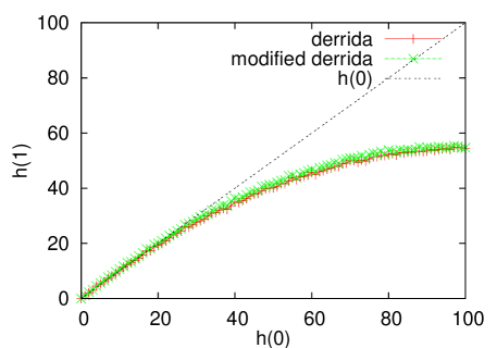
Figure 4: Derrida plot (+) and modified Derrida plot (x) of a network with $K=2$, $N=100$.

Finally, we checked the validity of the annealed approximation by comparing the Derrida plot obtained when starting from random initial states with the Derrida plot obtained when starting only from states that are on an attractor. In order to obtain initial states that are on an attractor, we started from a random state and ran the simulation until an attractor was reached. In this way, attractors are weighted by the size of their basin of attraction.

Within the annealed approximation, there is no concept of an attractor. An attractor is a periodic sequence of states, and it can only occur if the connections between nodes are fixed in time, and not annealed. Since an attractor contains only a small subset of all states, one might expect that the Derrida plot becomes different when the initial state is constrained to be on an attractor. We therefore evaluated a modified Derrida plot, where the initial state was an attractor state. Figure 4 shows the Derrida plot and the modified Derrida plot for a critical network of size $N=100$. The two curves agree very well with each other. We found an equally good agreement for frozen and chaotic networks. This result implies that states on attractors are “typical” states, which cannot be distinguished from transient states when evaluating the temporal behaviour of the Hamming distance.

III Networks evolved for robustness

In this section, we investigate the Derrida plot and its modifications for networks that were evolved for robustness of the dynamical attractors against perturbations of the node values. Like real networks, they are not random but shaped by their evolutionary history. We used networks evolved according to the rules described in previous work by two of the authors agnespaper , where the evolution of a single Boolean network is simulated by means of an adaptive walk. The adaptive walk is a hill climbing process that leads to a local fitness maximum and thus can yield insight into the fitness landscape of a system. In agnespaper , it was found that there is a huge plateau with the maximum fitness value that spans the network configuration space. Mutations change the connections and the update functions of the nodes. In the following, we describe the algorithm in more detail.

III.1 Algorithm used for the network evolution

The adaptive walk starts with a randomly created network. The fitness (that is the robustness) of this network is determined by the following procedure: First, the network is updated until it reaches an attractor. Then the value of each node is flipped one after the other, and it is counted how often the network returns to the same attractor and how many time steps this takes. The fitness value is the percentage of times the dynamics return to the given attractor after flipping a node, provided that the way back to the attractor takes on average no longer than two updates. If this condition is not fulfilled, the fitness is set to zero. After determining the fitness, a mutation is performed in the network. With equal probability, a connection between two nodes is added or deleted, a connection is redirected, or the Boolean function is changed. The mutation is accepted if it does not lower the fitness. The adaptive walk is continued until at least 15,000 accepted mutations have occurred. Since the networks reach maximum fitness after only a few evolutionary steps, most of these mutations are neutral (i.e., they do not change the fitness value), and the networks perform a random walk on the plateau of 100% fitness. The simulations are run for different $N$ up to $N=90$ and initial connectivities of $K_{ini}=1$ and $2$. Here we show representative networks with $N=11$, $50$ and $80$. For details on the algorithm, see agnespaper . In contrast to most simulations performed in that paper, we do not use canalyzing functions here, but the entire set of Boolean functions, as in the RBNs evaluated in the previous section.

III.2 General properties of evolved networks

We generated a set of evolved networks and evaluated first their structural and dynamical properties, which are briefly summarized in the following. The final networks have an average connectivity that is larger than 2 and therefore characteristic for the chaotic regime. The ensemble of evolved networks shows an average $K$ value of $3.1$ independently of the initial connectivity. Unlike the initial random networks, which have the same value of $K$ for all nodes, the evolved networks have a broad distribution of input connections, with a peak at 1 and an exponential decay for larger $K$. The distribution of output connections has not changed and is poissonian, as in random networks. The distribution of Boolean functions in the evolved networks is the same as for the initial networks, i.e., each function occurs with the same probability. We also evaluated the “sensitivity” $\lambda$ of the evolved networks, which is $K$ times the probability that a node changes its state when one of its inputs is changed Shmulevich04 . It is identical to the initial slope of the Derrida plot. We found $\lambda>1$, which also indicates that the final networks are in the chaotic regime. The large robustness of the evolved networks is due to a state space containing an attractor with a huge basin that comprises usually more than 90% of all possible states. Despite the high $K$ values, these networks show only short attractor lengths, mostly single-digit, with only a few active nodes on the attractors.

III.3 Derrida plots of evolved networks

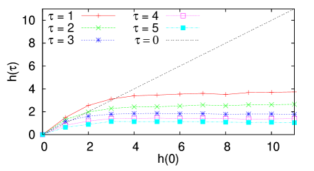
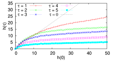
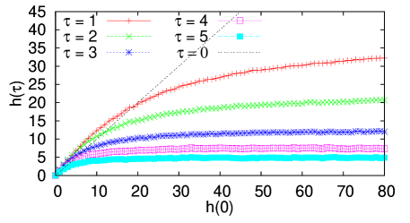
Figure 5: Generalized Derrida plots with $\tau$ = 1,2,3,4,5 of three networks that have been evolved for robustness. The parameters are $N=11$, $K=3.63$; $N=50$, $K=3.12$; $N=80$, $K=3.39$.

The Derrida plots and their generalized, iterated and modified versions are shown in figures 5 to 7 for three evolved networks of different sizes.

Figure 5 shows the generalized Derrida plots. They are clearly different from those of RBNs. For RBNs, the curves intersect all at the same point, which is a fixed point of the iterated Derrida maps. This fixed point value must be identical to 0.5 times the number of nonfrozen nodes, $N_{nf}$, in the stationary state, since each of these nodes change their state with probability 0.5 during one iteration. Since the iteration must converge to this fixed point, the generalized Derrida plots of RBNs approach with with increasing $\tau$ a step function with the value 0 at $h=0$ and with the fixed point value $0.5\cdot N_{nf}$ for all $h>0$ (see figure 3). This is in contrast to the evolved networks, where the maximum value reached by the curves decreases with increasing $\tau$, and so does the value of the fixed point of the map. Even though the initial states may be far from an attractor, the trajectories in state space experience constraints due to the fact that they are attracted to the same small part of the state space. The plot shows how with increasing $\tau$ more and more nodes freeze while the system approaches the attractor.

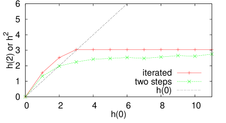
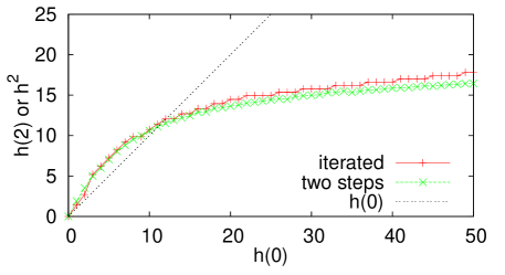
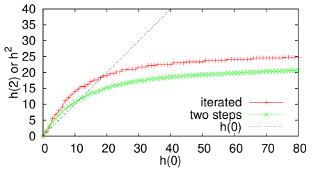
Figure 6: Generalized Derrida plot $h(2)$ (x symbols), and iterated Derrida map $h^{2}$ (+ symbols) of the three networks evolved for robustness $N=11$, $K=3.63$, $N=50$, $K=3.12$ and $N=80$, $K=3.39$.

Figure 6 shows the curves of the two-step Derrida plot and the iterated Derrida map for the same three networks. In contrast to RBNs (see figure 3), the corresponding curves of evolved networks do not agree with each other. The two-step Derrida plots are for larger $h$ values below the iterated Derrida map. This indicates again that trajectories do not move away from each other as fast as suggested by the first iteration.

Finally, in figure 7 we show the modified Derrida plot of the evolved networks. The initial slope of these plots is close to 1, which means that the networks appear to be critical for perturbations occurring on attractors. In contrast, the initial slope is larger than 1 for the conventional Derrida plot, which means that the evolved networks appear at first chaotic when starting from a random initial state. Such a decrease in the initial slope is plausible as these networks were evolved for stable attractors.

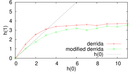
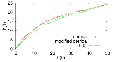
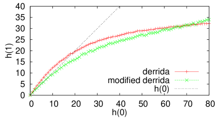
Figure 7: Derrida plot and modified Derrida plot of the three networks evolved for robustness $N=11$, $K=3.63$, $N=50$, $K=3.12$ and $N=80$, $K=3.39$.

We have shown here only the results for three networks. For other evolved networks, the qualitative behaviour of the curves that we just described is the same. The precise shape of the curves, however, differs between different networks of the same size.

All these results indicate that the state space structure of these evolved networks is fundamentally different from that of RBNs. They contain one large dominant attractor, which influences the Hamming distance between trajectories already during the first few time steps. The evolved networks combine features characteristic of the frozen phase (the very short attractor and the very small number of attractors), of the chaotic phase (the initial slope of the Derrida plot), and of the critical point (the initial slope of the modified Derrida plot, the large number of frozen nodes).

IV The yeast cell cycle network

(a)

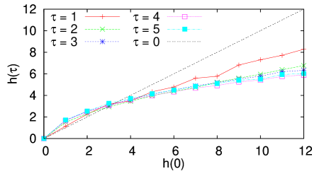
(b)

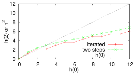
(c)

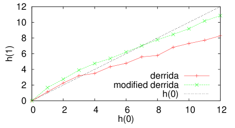
Figure 8: Generalized (top), iterated (middle, + symbols) and modified Derrida plot (bottom, x symbols) for the yeast cell-cycle network of Li et al. Li

Finally, we want to apply the different kinds of plots to a model of a real biological network. The model of the yeast cell-cycle network of Li et al. Li is known to show a highly robust behaviour. This robustness is due to the basin size of the main attractor rather than to a specific state space structure Willadsen . The model consists of 11 key nodes, and it has Boolean update rules based on threshold functions. A 12th node does not represent a protein, but the cell size. Depending on whether this size is below or above a threshold value, a new round of the cell cycle is initiated by turning on the 12th node. The main fixed point of the network, which attracts more than 80 percent of all network states, corresponds to the G1 phase of the cell cycle, during which the cell grows in size. The other attractors of the network are also fixed points.

The generalized, iterated and modified Derrida plots for this model are shown in figure 8. All three graphs show again clear deviations from the plots for RBNs. The generalized plots resemble those of a chaotic RBNs as far as the initial slope and the almost stationary fixed point is concerned, but for larger $h$ and higher iteration number the slope does not become horizontal as is the case for chaotic RBNs. This must be due to the influence of the large basin of attraction and to long transient times which prevent the system from showing any kind of stationary behaviour.

In contrast to the networks evolved for robustness, the two-step Derrida plot of the yeast cell-cycle network lies above the iterated Derrida map (figure 8 b). This indicates that the trajectories move away from each other faster than suggested by the first iteration. Similarly, the modified Derrida plot lies above the conventional one (see figure 8 c), showing that perturbations of attractor states have more impact than perturbations of random states. This fits together with the finding that the fixed point of the cell cycle is more sensitive to perturbations than other states of the model Fretter .

V Conclusion

In this paper, we introduced different generalizations of the Derrida plot and evaluated them for RBNs and for evolved BNs. We first showed that all the results obtained for RBNs agree with the annealed approximation, even when networks are small. In particular, RBNs satisfy equation (1), that allows us to predict the Derrida plots as long as the annealed approximation is valid. We then evaluated these plots for networks that were evolved for high robustness of their attractors by means of an adaptive walk. For those networks, the annealed approximation is no longer valid, and the temporal evolution of the Hamming distance between two network states is no longer determined by the value of the Hamming distance alone. Furthermore, the simulation results imply that the standard classification of the dynamics of Boolean networks into frozen, critical and chaotic behaviour can not be applied to evolved networks, since these networks show features characteristic of all three types of behaviour. Nevertheless the different kinds of Derrida plots shown in this paper allow a more detailed insight into the state space structure and therefore into the actual behaviour of the networks. We conclude that this simple classification may not be appropriate for biological networks either, since such networks are also shaped by their evolutionary history. Our work thus confirms and complements the work by Sevim and Rikvold sevim , who arrive at similar conclusions. Future studies of perturbation propagation in realistic BNs will have to focus on the question of how these networks achieve the remarkable combination of dynamical robustness with the ability to respond flexibly to changes in the environment.

We acknowledge partial support of this project by the Volkswagen Foundation and by the Deutsche Forschungsgemeinschaft (DFG contract no. Dr300/4-1.)

References

- (1) Rosen-Zvi M, Engel A and Kanter I 2001 Phys. Rev. Lett. 87 078101
- (2) Moreira A A, Mathur A, Diermeier D and Amaral L A N 2004 Proc. Natl Acad. Sci. USA 101 12085–90
- (3) Lagomarsino M C, Jona P and Bassetti B 2005 Phys. Rev. Lett. 95 158701
- (4) Bassler K E, Lee C and Lee Y 2004 Phys. Rev. Lett. 93 038101
- (5) Szejka A and Drossel B 2007 Eur. Phys. J. B 56 373–80
- (6) Herrmann H J 1988 Nonlinear Phenomena in Complex Systems ed A N Proto (Amsterdam: North-Holland) pp 151
- (7) Derrida B and Weisbuch G 1986 J. Physique 47 1297–303
- (8) Kauffman S A 1969 J. Theor. Biol. 22 437–67
- (9) Samuelsson B and Troin C 2003 Phys. Rev. Lett. 90 098701
- (10) Kaufman V, Mihaljev T and Drossel B 2005 Phys. Rev. E 72 046124
- (11) Sevim V and Rikvold P A 2008 J. Theor. Biol. 253 323–32
- (12) Li F, Long T, Lu Y, Ouyang Q and Tang C 2004 Proc. Natl. Acad. Sci. USA 101 4781–6
- (13) Derrida B and Pomeau Y 1986 Europhys. Lett. 1, 45–9
- (14) Kesseli J, Rämö B and Yli-Harja O 2006 Phys. Rev. E 74 046104
- (15) Aldana-Gonzalez M, Coppersmith S and Kadanoff L P 2003 Perspectives and Problems in Nonlinear Science, A celebratory volume in honor of Lawrence Sirovich ed E Kaplan, J E Mardsen and K R Sreenivasan (New York: Springer)
- (16) Shmulevich I and Kauffman S A 2004 Phys. Rev. Lett. 93 048701
- (17) Willadsen K and Wiles J 2007 J. Theor. Biol. 249 749–65
- (18) Fretter C and Drossel B 2008 Eur. Phys. J. B 62 365–71