Adjoint fermion zero-modes for SU(N) calorons

Abstract:

We derive analytic formulas for the zero-modes of the Dirac equation in the adjoint representation in the background field of $Q=1$ SU(N) calorons. Solutions with various boundary conditions are obtained, including the physically most relevant cases of periodic and anti-periodic ones. The latter are essential ingredients in a semi-classical treatment of finite temperature supersymmetric Yang-Mills theory. A detailed discussion of adjoint zero-modes in several other contexts is also presented.

1 Introduction

In recent years there has been renewed interest in the study of gauge theories on $R^{3}\times S^{1}$ in situations that could be amenable to semi-classical treatment. This refers not only to thermal QCD but also to other QCD-like theories seemingly exhibiting exotic phase diagrams which depend on the representation and the boundary conditions for the fermionic fields. As an example, arguments are given to support the idea that adjoint QCD remains confined for any value of the $S^{1}$ cycle when fermions are endowed with periodic boundary conditions [1]-[6]. This temperature independence, interpreted in the spirit of the Eguchi-Kawai reduction [7], could allow for an analytical approach to confinement in this theory. Here, as well as in ordinary thermal QCD or in supersymmetric gluodynamics, the relevant semi-classical objects are BPS monopoles and finite temperature instantons (calorons). Remarkably, these two objects cannot be considered as independent entities. For non-trivial values of the Polyakov loop at infinity and high temperatures, calorons split into N (for SU(N)) constituent BPS monopoles [8]-[11], with the well known Harrington-Shepard caloron [12] corresponding to the case in which N-1 of them become massless. Non-trivial holonomy calorons provide therefore a particular realisation of the idea of instanton quarks [13]-[15], instrumental to many semi-classical attempts at explaining confinement in QCD. Constituent monopoles within calorons have been successfully used for obtaining, yet another, weak coupling computation of the gluino condensate in 4D ${\cal N}=1$ supersymmetric Yang-Mills theory [1]. The success of this approach relies on the relevance of non-trivial holonomy configurations when the theory is defined on $R^{3}\times S^{1}$ with periodic boundary conditions for the adjoint fermions. On the contrary, in thermal QCD an old one-loop result by Gross, Pisarski and Yaffe [16] indicates the thermodynamic suppression of such configurations and consequently seems to point towards the irrelevance of non-trivial holonomy calorons for finite temperature QCD. Nevertheless, this result has recently been challenged on the basis of non-perturbative calculations [17] and lattice simulations [18]. Although the issue is far from being settled, see e.g. [19], it has revived the interest in applying semi-classical techniques to the analysis of QCD in a thermal set up. Last but nor least, non-trivial holonomy calorons could as well be of relevance for settling issues at stake such as that of supersymmetry breaking at finite temperature [20]-[26], or the previously discussed phase structure of adjoint QCD or other QCD-like gauge theories.

An essential ingredient in the semi-classical analysis of these theories are the zero-modes of the Dirac operator in the background of the caloron gauge field. Those in the fundamental representation have been previously obtained, first for $Q=1$ SU(2) calorons [27], and later generalised for SU(N) [28]. Remarkably they are supported on a single BPS monopole selected through the choice of boundary conditions for the fermions on the thermal cycle. In the present paper we will focus on the derivation of the zero-modes of the Dirac operator in the adjoint representation, relevant for supersymmetric gluodynamics as well as for adjoint QCD. The corresponding expressions for $Q=1$ SU(2) calorons have been obtained in Refs. [29] and [30] for fermions with periodic and anti-periodic boundary conditions in time. Here we will generalise those formulas to gauge group SU(N).

Let us finally mention that adjoint zero-modes have also interest in the context of using eigenstates of the Dirac operator to trace topological structures in the QCD vacuum. In particular, the use of the so called supersymmetric zero-mode, whose density profile matches that of the gauge action density, has been advocated by one of the present authors in Ref. [31]. First successful tests of the proposal were presented both there and in Ref. [32].

The paper is organised as follows. Sections 2 to 4 deal with the general construction of the adjoint zero-modes (the reader interested only in the specific solutions for the calorons could go directly to section 6). In section 2 we introduce some basic properties of adjoint zero-modes and discuss their relation to self-dual deformations of the gauge field. The derivation of the zero-modes relies heavily on the ADHM formulation for self-dual solutions of the classical equations of motion which is revised in section 3. There we also describe the general construction of the adjoint modes as deformations of the ADHM gauge field. The ADHM formalism has been devised to provide self-dual gauge fields on the sphere or $R^{4}$. To deal with more general manifolds one can make use of the Nahm-ADHM formalism. A general introduction is presented in section 4, starting with the simplest case of the 4-torus. We discuss there how the Nahm transform provides a mapping between the original self-dual gauge field and a self-dual gauge field living on the dual torus. We show how the adjoint zero-modes of the original Dirac operator are mapped onto those of the dual Dirac operator. In some cases the latter is much simpler than the original one and the Dirac equation can be easily solved. This constitutes the basis of the construction. It provides adjoint zero-modes with periodic boundary conditions in time. Anti-periodic modes are derived by making use of the so called replica trick which is described in section 4.1. The idea is to replicate the original thermal cycle and solve for the Dirac equation on the replicated torus. The periodic zero-modes thus obtained can be easily decomposed into periodic and anti-periodic zero-modes for the original, unreplicated torus. The application of these ideas to the case of calorons is presented in section 5. Explicit solutions for periodic and anti-periodic zero-modes are derived in section 6 where we also discuss the generalisation of our formulas to other periodicity conditions for the adjoint fermions. Section 7 presents some illustrative examples and discusses in detail some general properties of the solutions such as periodicity, normalisability and concordance with the expected number of zero-modes as dictated by the index theorem. Finally, we end in section 8 with a brief summary of the results and a recollection of possible applications. The most technical details concerning the derivation of the adjoint zero-modes in sections 5 and 6 are deferred to an Appendix.

2 Generalities about adjoint zero-modes

Our goal is that of studying euclidean adjoint fermionic zero-modes in the background field of SU(N) calorons. In this section we will revise a set of basic facts about adjoint modes. They are solutions of the equation

$$\gamma_{\mu}D_{\mu}\psi=0\,,$$ (1)

where the covariant derivative $D_{\mu}=\partial_{\mu}-iA_{\mu}$ is expressed in terms of the gauge potential $A_{\mu}$. This equation factorises into two Weyl equations for the two chiral components. The equation for the left-handed (or positive chirality $\gamma_{5}\psi=\psi$) component is

$$\overline{\sigma}_{\mu}D_{\mu}\psi_{+}=0\,,$$ (2)

where the Weyl matrices are $\overline{\sigma}_{\mu}=(\mathbf{I},i\vec{\tau})$, and $\tau_{i}$ are the Pauli matrices. Multiplication formulas with the adjoint Weyl matrices ($\sigma_{\mu}=(\mathbf{I},-i\vec{\tau})$)

$$\sigma_{\mu}\overline{\sigma}_{\nu}=\eta^{\mu\nu}_{\alpha}\overline{\sigma}_{\alpha}$$ (3)

$$\overline{\sigma}_{\mu}\sigma_{\nu}=\bar{\eta}^{\mu\nu}_{\alpha}\sigma_{\alpha}$$ (4)

define the real ‘t Hooft symbols $\eta^{\mu\nu}_{\alpha}$.

All the former equations are valid for all gauge groups and any representation. This dependence is hidden in the form of

$$A_{\mu}=\sum_{a}A_{\mu}^{a}T^{(R)}_{a}\,,$$ (5)

where $a$ runs over the generators of the group and the matrices $T^{(R)}_{a}$ are their expression in representation $R$. In the adjoint representation the generators $(T_{a})_{bc}=-if_{abc}$ are expressed in terms of the structure constants of the group $f_{abc}$. Thus, the covariant derivative $D_{\mu}^{ab}$ is real. This, together with the definition of $\overline{\sigma}_{\mu}$ implies that given one solution $\psi_{+}$ one can construct a linearly independent one $\psi_{+C}$. In components

$$\psi^{a}_{+}=\pmatrix{\kappa^{a}_{1}\cr\kappa^{a}_{2}}\longrightarrow\psi_{+C}^{a}=\pmatrix{-\overline{\kappa}_{2}^{a}\cr\overline{\kappa}_{1}^{a}}=\sigma_{2}\overline{\psi}^{a}_{+}\,,$$ (6)

where the bar denotes complex conjugation. Notice that the two vectors form the two columns of a $2\times 2$ matrix $\Psi^{a}=(\psi^{a}_{+},\psi_{+C}^{a})$. This type of matrices define a representation of the field of quaternions, and from now on we will make no distinction among both sets. In this notation any linear combination of $\psi_{+}^{a}$ and $\psi_{+C}^{a}$ can be simply represented by the multiplication by an arbitrary constant quaternion $Q$ on the right

$$\Psi^{a}\longrightarrow\Psi^{a}Q\,.$$ (7)

The density is the same for all vectors in this space.

Self-dual gauge fields $A_{\mu}^{a}$ are those for which the field strength $F_{\mu\nu}=i[D_{\mu},D_{\nu}]$ satisfies

$$\bar{\eta}^{\mu\nu}_{i}F_{\mu\nu}=0\,,$$ (8)

for all $i=1,2,3$. In analysing the solutions of the Weyl equations for self-dual gauge fields, it is important to consider the possible zero-modes $\kappa(x)$ of the covariant Laplacian $D_{\mu}D_{\mu}$. It is clear that the only zero-modes are functions that are simultaneously annihilated by all the $D_{\mu}$ ($D_{\mu}\kappa(x)=0$). This implies that

$$[F_{\mu\nu}(x),\kappa(x)]=0\,.$$ (9)

Except for very particular abelian-like gauge fields, this equation will have no solution other than the trivial one $\kappa(x)=0$. From this result it is easy to conclude that the right-handed Weyl equation will have no zero-modes. From here one can make use of the index theorem [33] to extract the number of zero-modes of the left-handed Weyl equation. Notice also, that the absence of zero-modes would guarantee the invertibility of the covariant Laplacian.

Another very important result concerning adjoint zero-modes of self-dual gauge fields is to realise the connection among self-dual deformations and solutions of the left-handed Weyl equation. Given a self-dual deformation $\delta A_{\mu}$, one can choose a representative within the gauge trajectory satisfying the background gauge condition

$$D_{\mu}\delta A_{\mu}=0\,.$$ (10)

The existence and uniqueness (up to non-trivial gauge transformations not connected with the identity) of this representative relies on the invertibility of the covariant Laplacian. Now, it is simple to see that the condition of self-duality, plus the background gauge condition amount to

$$\overline{\sigma}_{\mu}D_{\mu}\Psi=0\,,$$ (11)

where $\Psi=\delta A_{\mu}\sigma_{\mu}$. The relation works both ways, so that there is a one-to-one correspondence between self-dual deformations and left-handed zero-modes. This relation combined with the index theorem was used in Refs. [34] to count the (dimensionality) number of moduli parameters of the manifold of self-dual gauge fields.

Notice that if we transform one solution of Eq. (11) by right multiplication by a quaternion $\Psi\longrightarrow\Psi Q$ the corresponding deformation transforms as

$$\delta A_{\mu}\longrightarrow q_{\nu}\bar{\eta}^{\mu\rho}_{\nu}\delta A_{\rho}=q_{\nu}\eta^{\nu\rho}_{\mu}\delta A_{\rho}\,,$$ (12)

where $Q=q_{\mu}\overline{\sigma}_{\mu}$.

A particular class of deformations is associated to symmetries (conformal transformations of the metric) that do not leave the solution invariant. Particularly interesting is the case of translations. Translation in the $\rho$ direction gives a deformation $\partial_{\rho}A_{\mu}$, which in general does not satisfy the background field gauge. However, if we write

$$\delta A_{\mu}=\partial_{\rho}A_{\mu}+D_{\mu}(-A_{\rho})=F_{\rho\mu}\,,$$ (13)

the gauge condition is satisfied. This gives rise to the famous supersymmetric zero-mode present in conformally flat manifolds.

3 ADHM construction of adjoint zero-modes

In this section we will revise the main formulas of the ADHM construction [35] of self-dual gauge fields, and in particular the expression of adjoint zero-modes. We will restrict ourselves to the case of gauge group SU(N).

The ADHM expression for an SU(N) gauge field with topological charge $Q$ is given by:

$$A_{\mu}(x)=iN^{\dagger}\partial_{\mu}N\,,$$ (14)

where $N$ is a $(2|Q|+N)\times N$ matrix satisfying $N^{\dagger}N=I\!\!I_{N}$. This vector is annihilated by the $(2|Q|+N)\times 2|Q|$ matrix $M$:

$$N^{\dagger}M=0\,.$$ (15)

The second index of the matrix $M$ is split into a index running from 1 to $|Q|$ and an spinorial index $\alpha=1,2$. This matrix has the form:

$$M=A+B\hat{x}\,,$$ (16)

where $A$ and $B$ are constant matrices of the same type as $M$, and $\hat{x}=x_{\mu}\sigma_{\mu}$ is an $x$-dependent quaternion which acts on the spinorial index.

One can show that $A_{\mu}$ constructed in such a way is self-dual provided the matrix $R=M^{\dagger}M$ is invertible and commutes with the $\sigma_{\mu}$. Let us find out the implications of this condition for the matrices $A$ and $B$. We have that both $B^{\dagger}B$ and $A^{\dagger}A$ must commute with $\sigma_{\mu}$, and the matrix $B^{\dagger}A$ can be written as $S_{\mu}\sigma_{\mu}$ with $S_{\mu}$ hermitian. To express this equation in a more compact way we might introduce some notation, which will turn out to play an important role in what follows.

Given a $2m\times 2m$ matrix $S=S_{\mu}\sigma_{\mu}$, where $S_{\mu}$ are $m\times m$ complex matrices, we denote

$$\overline{S}=S_{\mu}\overline{\sigma}_{\mu}$$

The overline operation combined with the hermitian conjugate is a particularly interesting operation (star-operation):

$$S^{\star}\equiv\overline{S^{\dagger}}=S_{\mu}^{\dagger}\sigma_{\mu}\,,$$ (17)

which will turn out to be very useful in what follows. In particular, it satisfies

$$(SQ)^{\star}=S^{\star}Q\,,$$ (18)

$$(QS)^{\star}=QS^{\star}\,,$$ (19)

for any square matrix with quaternionic entries $S$, and an arbitrary quaternion $Q$. From here it follows, in the particular case of $2\times 2$ matrices (m=1), that $(TS)^{\star}=T^{\star}S^{\star}$. The subspace of quaternions is characterised by the condition $Q^{\star}=Q$. Furthermore, if the $2\times 2$ matrix is of dyadic form $S=\xi\zeta^{\dagger}$, then

$$S^{\star}=\xi_{C}\zeta_{C}^{\dagger}\,,$$ (20)

where the subscript $C$ stands for the “charge-conjugate” introduced in the last section.

Using the previous notation, we can rewrite the ADHM conditions as

$$(B^{\dagger}A)^{\star}=B^{\dagger}A\,,$$ (21)

and

$$(M^{\dagger}M)^{\star}=M^{\dagger}M\,.$$ (22)

This type of equations will appear several times along the paper. If we write as before $S=S_{\mu}\sigma_{\mu}$, the condition $S^{\star}=S$ amounts to $S_{\mu}=S_{\mu}^{\dagger}$.

Another relation which plays an important role in the following derivations is that, given an arbitrary $2|Q|$ square matrix $S=S_{\mu}\sigma_{\mu}$, one obtains

$$\sigma_{\mu}S\sigma_{\mu}=\overline{\sigma}_{\mu}S\overline{\sigma}_{\mu}=-2\overline{S}\,.$$

Using this relation we can show that

$$(\partial_{\mu}(M^{\dagger}M)+(\partial_{\mu}M^{\dagger})M)\overline{\sigma}_{\mu}=0\,.$$ (23)

This formula will be important later. The proof is simple. We plug in the expression for $M$ and perform the derivatives and obtain:

$$2\overline{\sigma}_{\mu}(B^{\dagger}M)\overline{\sigma}_{\mu}+M^{\dagger}B\sigma_{\mu}\overline{\sigma}_{\mu}\,.$$

Using $\sigma_{\mu}\overline{\sigma}_{\mu}=4$ and Eq. (22) one easily verifies that it vanishes.

Let us now proceed to study the zero-modes of the Dirac operator in terms of the ADHM quantities introduced above. The expression for the normalised zero-modes in the fundamental representation, derived in Ref. [36], is given by:

$${\boldsymbol{\psi}}=\frac{1}{\pi}N^{\dagger}BR^{-1}\tau_{2}\,(B^{\dagger}B)^{1\over 2}.$$ (24)

The quantity ${\boldsymbol{\psi}}$ is a $N\times 2Q$ matrix, with the first index being the ordinary colour index. The second index decomposes into an spinorial one, and another labelling the $Q$ different linearly independent solutions, in agreement with the index theorem.

The adjoint zero-modes can be derived by exploiting their relation with self-dual deformations. These can be obtained by deforming the matrix $M$ and the vector $N$ of the ADHM construction [37]. It takes the form

$$\delta A_{\mu} = i\delta N^{\dagger}\partial_{\mu}N+iN^{\dagger}\partial_{\mu}\delta N\,,$$ (25)

$$\delta N^{\dagger}M = -N^{\dagger}\delta M\,,$$ (26)

$$\delta N^{\dagger}N+N^{\dagger}\delta N = 0\,.$$ (27)

Given a deformation $\delta M$, the variation of $\delta N$ is determined from Eq. (26). The solution is not unique since the left-kernel of $M$ is non-trivial. This allows us to choose a solution $\widetilde{\delta}N$ satisfying

$$\widetilde{\delta}N^{\dagger}N=0\,,$$ (28)

which is also compatible with Eq. (27). A general solution would then be

$$\delta N=\widetilde{\delta}N-iN\omega\,,$$ (29)

with $w$ a hermitian matrix. Using the form of the orthogonal projector to the kernel of M:

$$P=MR^{-1}M^{\dagger}\,,$$ (30)

we might write

$$\widetilde{\delta}N^{\dagger}=\widetilde{\delta}N^{\dagger}P=-N^{\dagger}\delta MR^{-1}M^{\dagger}\,.$$ (31)

Plugging this expression into Eq. (25) we arrive at:

$$\widetilde{\delta}A_{\mu}=iN^{\dagger}\left(\delta MR^{-1}\partial_{\mu}M^{\dagger}-\partial_{\mu}MR^{-1}\delta M^{\dagger}\right)N\equiv iN^{\dagger}(H_{\mu}-H^{\dagger}_{\mu})N\,,$$ (32)

where we have moved the partial derivatives around in an obvious way. If instead of this solution we would have used the general one Eq. (29), the result would be

$$\delta A_{\mu}=\widetilde{\delta}A_{\mu}+D_{\mu}\omega\,,$$ (33)

a gauge transform of the previous one. The quantity $H_{\mu}$ appearing in Eq. (32) can be written as

$$H_{\mu}=\delta M\overline{\sigma}_{\mu}R^{-1}B^{\dagger}\,.$$ (34)

From here it is clear, by using the formula

$$\overline{\sigma}_{\nu}\overline{\sigma}_{\mu}=\eta^{\nu\rho}_{\mu}\overline{\sigma}_{\rho}\,,$$ (35)

that multiplying $\delta M$ on the right by an arbitrary quaternion $Q=q_{\nu}\overline{\sigma}_{\nu}$ transforms the deformation as in Eq. (12), namely another one corresponding to the 2-dimensional space of adjoint zero-modes mentioned in the previous section.

We have obtained the expression of the self-dual deformation in terms of $\delta M$, the deformation of the $M$ matrix. Notice that these deformations are not arbitrary, but should preserve the form $\delta M=\delta A+\delta B\hat{x}$ and preserve the invertibility (trivial) and the condition of commuting with quaternions. The latter condition can be re-expressed as

$$T-T^{\star}=\overline{T-T^{\star}}\,,$$ (36)

where $T=M^{\dagger}\delta M$.

Now we should verify whether Eq. (32) satisfies the background gauge condition. Acting with the covariant derivative and after some algebra we obtain

$$D_{\mu}\widetilde{\delta}A_{\mu}=i4N^{\dagger}\left(\,\delta B\,R^{-1}B^{\dagger}-BR^{-1}\delta B^{\dagger}-BR^{-1}(M^{\dagger}\delta M-\delta M^{\dagger}M)_{0}R^{-1}B^{\dagger}\right)N\,,$$ (37)

where the sub-index $0$ amounts to extracting the part commuting with quaternions:

$$(S)_{0}\equiv\frac{1}{2}(S+\overline{S})=\frac{1}{4}\sigma_{\mu}S\overline{\sigma}_{\mu}\,.$$ (38)

We leave to the reader the details of reaching to Eq. (37). As an aid, we mention that we have used the form of the matrices $M$ and $\delta M$, the previous relations Eq. (23) and Eq. (38), and the following formula for the covariant derivative of an object of the form $\omega=N^{\dagger}HN$:

$$D_{\mu}\omega=N^{\dagger}\partial_{\mu}\left((I\!\!I-P)H(I\!\!I-P)\right)N=$$

$$N^{\dagger}\left(\partial_{\mu}H-\partial_{\mu}MR^{-1}M^{\dagger}H-HMR^{-1}\partial_{\mu}M^{\dagger}\right)N\,.$$ (39)

From Eq. (37), we conclude that the covariant derivative vanishes provided:

$$\delta B\,R^{-1}B^{\dagger}-BR^{-1}\delta B^{\dagger}=0\,,$$ (40)

$$(M^{\dagger}\delta M-\delta M^{\dagger}M)_{0}=0\,.$$ (41)

The last equation can be combined with the condition on the deformations $\delta M$, Eq. (36), to conclude:

$$T=T^{\star}\,,$$ (42)

where $T=M^{\dagger}\delta M$.

Up to now we have not used the freedom to redefine $M$ without altering the form of the gauge field $A_{\mu}$. There are two types of transformations of this kind. The first is to replace $M\longrightarrow ML$ with invertible, constant and commuting with quaternions $L$. The second transformation is to modify $M\longrightarrow VM$ with $V$ unitary and constant. The same transformation has to be done to $N$ ($N\longrightarrow VN$). Using these transformations Christ, Weinberg and Stanton [38] were able to show that the $M$ matrix can be brought to the following canonical form:

$$M=\pmatrix{q^{\dagger}\cr\widetilde{A}-\hat{x}}\,.$$ (43)

Then we have

$$N=\pmatrix{I\!\!I_{N}\cr-u}F^{-1/2}\,,$$ (44)

where $u$ is given by

$$u\equiv\widetilde{M}^{-1\dagger}q=B^{\dagger}NF^{1/2}\,,$$ (45)

with $\widetilde{M}=\widetilde{A}-\hat{x}$. The $N\times N$ matrix $F$ is fixed by the normalisation condition ($N^{\dagger}N=I\!\!I_{N}$):

$$F=I\!\!I_{N}+u^{\dagger}u\,.$$ (46)

We will now give the expression of the gauge field and the vector potential in this canonical form. Introducing $\omega=R^{-1}q$, one can show that

$$u=\widetilde{M}\omega F\,.$$ (47)

Another useful expression is

$$R^{-1}u=\frac{1}{2}(\hat{\partial}R^{-1})qF=\frac{1}{2}\hat{\partial}\omega F\,,$$ (48)

where $\hat{\partial}\equiv\sigma_{\mu}\partial_{\mu}$.

With this notation the main expressions for the ADHM fields are given by:

$$F^{1/2}A_{\mu}(x)F^{1/2}=iu^{\dagger}\partial_{\mu}u-iF^{1/2}\partial_{\mu}F^{1/2}\equiv F^{1/2}{\cal A}_{\mu}F^{1/2}-iF^{1/2}\partial_{\mu}F^{1/2}\,,$$ (49)

where

$${\cal A}_{\mu}=\frac{i}{2}F^{1/2}q^{\dagger}\bar{\sigma}^{\mu}\hat{\partial}\omega F^{1/2}\,.$$ (50)

The (chromo-)electric field is given by

$$E_{i}=-F^{-1/2}u^{\dagger}\tau_{i}\hat{\partial}\omega F^{1/2}\,,$$ (51)

and the zero-modes of the Dirac operator in the fundamental representation by:

$${\boldsymbol{\psi}}=\frac{1}{2\pi}F^{1/2}\left(\hat{\partial}\omega\right)^{\dagger}\tau_{2}.$$ (52)

Now we go back to our main goal of obtaining the adjoint zero-modes. Notice that $\delta B=0$ so that the first condition implying the background gauge Eq. (40) is automatically satisfied. The form of the self-dual deformation can be obtained by using

$$\delta M^{\dagger}\,N=(\delta q-\delta\widetilde{A}^{\dagger}u)F^{-1/2}\,,$$ (53)

and replacing it in our general formula Eq. (32):

$$\delta A_{\mu}=\frac{i}{2}F^{-1/2}(\delta q^{\dagger}-u^{\dagger}\delta\widetilde{A)}\bar{\sigma}^{\mu}\hat{\partial}\omega F^{1/2}+h.c.\,.$$ (54)

The condition that this is a self-dual deformation in the background Lorentz gauge, is simply Eq. (42) where

$$T\equiv M^{\dagger}\delta M=q\delta q^{\dagger}+\widetilde{A}^{\dagger}\delta\widetilde{A}-\bar{x}\delta\widetilde{A}\,.$$ (55)

The part proportional to $\bar{x}$ must satisfy the equation by itself ($\delta\widetilde{A}=(\delta\widetilde{A})^{\star}$). The remaining part can be rewritten as

$$\widetilde{A}^{\dagger}\delta\widetilde{A}-(\widetilde{A}^{\dagger}\delta\widetilde{A})^{\star}=-q\delta q^{\dagger}+(q\delta q^{\dagger})^{\star}\,.$$ (56)

4 Nahm-ADHM formalism

The ADHM formalism is valid for gauge fields on the sphere or in $R^{4}$ with appropriate boundary conditions at infinity. For other manifolds one can use the extension introduced by Nahm [39]. A particularly symmetric case is that of the 4-torus $T^{4}$. Essentially, one can embed the torus onto $R^{4}$ and impose the appropriate periodicity conditions. If we look at the torus configurations as solutions in $R^{4}$, it is clear that their topological charge $Q$ would be infinite. Then one can interpret the corresponding matrix indices of the basic ADHM quantities, $M=A+B\hat{x}$ and $N$, as Fourier coefficients of functions or operators depending on 4 new dual coordinates $z_{\mu}$. In particular, the matrix $B$ can be chosen as minus the identity operator ($B=-I\!\!I$) and $A=\hat{D}_{\mu}\sigma_{\mu}/(2\pi i)$. The Nahm-dual covariant derivative $\hat{D}_{\mu}$ is given by

$$\hat{D}_{\mu}=\frac{\partial}{\partial z_{\mu}}-i\hat{A}_{\mu}(z)\,,$$ (57)

expressed in terms of the Nahm-dual gauge field $\hat{A}_{\mu}(z)$. The operator $A^{\dagger}$ becomes simply proportional to the Nahm-dual left-handed Weyl operator in the fundamental representation, and $N$ is replaced by the zero-modes $\hat{\boldsymbol{\psi}}(z,x)$ of the modified Weyl equation

$$\overline{\sigma}_{\mu}(\hat{D}_{\mu}-2\pi ix_{\mu})\hat{\boldsymbol{\psi}}(z,x)=0\,.$$ (58)

With this interpretation all the standard ADHM conditions and formulas adopt a simple interpretation. For example, the condition that $R$ commutes with quaternions, leads to the self-duality of the Nahm-dual gauge field. The Weitzenböck formula then gives

$$R=-\frac{\hat{D}_{\mu}\hat{D}_{\mu}-4\pi ix_{\mu}\hat{D}_{\mu}-4\pi^{2}x^{2}}{4\pi^{2}}\,,$$ (59)

which obviously commutes with quaternions. Its invertibility follows from the invertibility of the covariant Laplacian in Nahm-dual space.

The formulas work both ways, so that the Nahm-dual field can be obtained from the original self-dual field by the standard formula

$$\hat{A}_{\mu}(z)=i\int dx\,{\boldsymbol{\psi}}^{\dagger}(x,z)\frac{\partial}{\partial z_{\mu}}{\boldsymbol{\psi}}(x,z)\,,$$ (60)

in terms of the normalised zero-modes ${\boldsymbol{\psi}}(x,z)$ of the modified Weyl equation in the fundamental representation:

$$\overline{\sigma}_{\mu}(D_{\mu}-2\pi iz_{\mu}){\boldsymbol{\psi}}(x,z)=0\,.$$ (61)

These zero-modes can also be expressed in terms of Nahm-dual quantities by replacing in Eq. (24) the quantities by their equivalents

$${\boldsymbol{\psi}}(x,z)=-\frac{e^{2\pi izx}}{\pi}\int d^{4}z^{\prime}\,\hat{{\boldsymbol{\psi}}}^{\dagger}(z^{\prime},x)\hat{G}(z^{\prime},z;x)\tau_{2}$$ (62)

where $\hat{G}(z^{\prime},z;x)$ is the Green function of the operator $R$.

In Eq. (60) we have omitted the indices labelling the different solutions of the Weyl equation. The index theorem tells us that there are $Q$ linearly independent solutions, implying that $\hat{A}_{\mu}(z)$ is an SU(Q) gauge field. It can be shown that the new field has topological charge $N$. Thus, we obtain a mapping between SU(N) and SU(Q) self-dual gauge fields, which is an involution [40]. The Nahm-dual gauge field lives in the dual torus, parametrised by $z_{\mu}$, whose periods are the inverse of those that define the original torus.

Considering deformations, the aforementioned mapping implies $\delta M=-\delta\hat{A}_{\mu}\sigma_{\mu}/2\pi$. Plugging this onto Eq. (42) we get

$$\bar{\sigma}_{\mu}\hat{D}_{\mu}\hat{\Psi}=0\,,$$ (63)

where $\hat{\Psi}=\sigma_{\mu}\delta\hat{A}_{\mu}$, which is the left-chirality adjoint Dirac equation. Thus, adjoint zero-modes map onto adjoint Nahm-dual zero-modes and viceversa. A explicit formula can be read off from Eq. (32):

$$\delta A^{ij}_{\mu}(x)=\frac{i}{2}\int d^{4}z\,e^{-2\pi izx}\,{\boldsymbol{\psi}}^{ia}(x,z)\tau_{2}\sigma_{\mu}\overline{\sigma}_{\nu}\delta\hat{A}^{ab}_{\nu}(z)\hat{{\boldsymbol{\psi}}}^{bj}(z,x)+\mbox{\rm h. c.}$$ (64)

where colour ($i=1\ldots N$) and dual-colour ($a=1\ldots Q$) indices are explicitly shown and repeated indices summed over (spinorial indices are not displayed).

All general properties of the ADHM construction are preserved, and in particular the fact that the mapping operates among the 2-dimensional spaces formed by each mode and its CP transform.

4.1 Replicas

There are a set of interesting relations which arise by embedding a self-dual solution on the 4-torus onto that of a replicated torus with periods being multiples of the original one. We call the new solution a replicated solution or replica. The replicated solution has a topological charge which is a multiple of the topological charge of the original one $Q$. Consider for example replicating the solution in one direction by a factor $L$, then the topological charge of the replica is $QL$. If we now take the Nahm transform of this solution it corresponds to an SU(LQ) self-dual configuration. How does this solution relate to the Nahm transform of the original configuration? This question was addressed an answered in a previous paper by one of the authors [41]. The answer is the following one:

$$\hat{A}^{R}_{\mu}(z)={\rm diag}\{\hat{A}_{\mu}(z),\hat{A}_{\mu}(z+\frac{1}{L}),\ldots,\hat{A}_{\mu}(z+\frac{L-1}{L})\}\,,$$ (65)

where the symbol diag constructs an $L\times L$ diagonal matrix with its arguments. An important point to take into account is that the Nahm transform of the replicated solution lives in a torus (the dual-torus) which is a fraction $\frac{1}{L}$ of the size of that of the original one. The transition matrices can be read off from Eq. (65). In particular, if $\hat{A}_{\mu}(z)$ is strictly periodic with period 1, we have

$$\hat{A}^{R}_{\mu}(z+\frac{1}{L})=P\hat{A}^{R}_{\mu}(z)P^{\dagger}\,,$$ (66)

where $P$ is the $L\times L$ ‘t Hooft matrix ($P_{ij}=\delta_{j\,i+1}$).

Adjoint zero-modes of the Dirac equation in the background field of the replicated solutions can be derived once again from self-dual deformations satisfying Eq. (42). They are connected to deformations of the SU(LQ) Nahm transform satisfying the left-chirality adjoint Dirac equation on the dual-torus, i.e. Eq. (63). The adjoint zero-modes derived in this way are periodic in the replicated torus but do not necessarily satisfy the same boundary conditions on the original one. If applied to doubly replicated tori ($L=2$), this trick allows to obtain adjoint zero-modes which are anti-periodic in one direction. This technique was successfully applied in our previous paper [30] to obtain adjoint zero-modes of the Dirac equation in the background of SU(2) calorons. Here we will extend the derivation to general group SU(N).

5 Application for SU(N) calorons

In this section we will modify the previous formalism to make it valid for the case of calorons. These are self-dual gauge fields living in $R^{3}\times S^{1}$. The non-compact directions introduce modifications to the Nahm construction on the torus, which we will now specify. If we try to construct the Nahm-dual gauge field by the same formulas as before, we should study the solutions of the Weyl equation in the fundamental representation:

$$\overline{\sigma}_{\mu}(D_{\mu}-2\pi iz_{\mu}){\boldsymbol{\psi}}(x,z)=0\,.$$ (67)

The non-compactness of the spatial directions is helpful in trivialising the dependence of ${\boldsymbol{\psi}}(x,z)$ on $z_{i}$, which reduces to simple phase factors of the form $\exp(2\pi ix_{i}z_{i})$. With this, the Nahm-dual gauge field $\hat{A}_{\mu}(z)$ depends on a single variable $z_{0}$. There is, however, a problem that arises at specific values of $z_{0}$ for which some of the zero-modes become non-normalisable. This case depends on how fields decay at large distances and this is related to the holonomy. The latter is characterised by the eigenvalues of the Polyakov loop at spatial infinity, i.e.:

$$P_{\infty}=\exp\{i\,2\pi\,{\rm diag}(Z_{1},Z_{2},\cdots,Z_{N})\}\,,\quad{\rm with}\,\,0\leq Z_{1}\leq Z_{2}\leq\cdots Z_{N}<1,\,\,\sum_{a=1}^{N}Z_{a}\in\mathcal{Z}\,,$$ (68)

where we have made use of gauge invariance to bring the Polyakov loop to diagonal form and order the $Z_{a}$ in increasing values from 0 to 1. Indeed, non-normalisable solutions can only occur when $z_{0}$ coincides with one of the $Z_{a}$. Since the Nahm construction is local this means that the Nahm-dual fields would be self-dual except at these isolated points in $z_{0}$ [8], [9].

5.1 Nahm data for Q=1 calorons

The case of $Q=1$ calorons is particularly simple, since then the Nahm-dual field $\hat{A}_{\mu}(z)$ is abelian and, as already mentioned, depends on a single variable $z_{0}\equiv z$. It is furthermore periodic with period 1.

In this case, the whole scheme can be fitted into the ADHM formalism by identifying, the matrix $\widetilde{A}$, appearing in the Christ-Stanton-Weinberg canonical form, with the Weyl-Dirac operator associated to the Nahm-dual field:

$$\widetilde{A}=\frac{1}{2\pi i}\left(\partial_{z}-i\sigma_{\mu}\hat{A}_{\mu}(z)\right)\,.$$ (69)

Since the Nahm-dual gauge field is self-dual except when $z$ equals one of the $Z_{a}$, the ADHM condition of commutation of $R$ with the quaternions, can be interpreted as the condition of self-duality of $\hat{A}_{\mu}(z)$ up to delta function singularities at $Z_{a}$. These follow from the $q(z)$ having the form:

$$q(z)=\sum_{b=1}^{N}\delta(z-Z_{b})\,\zeta^{b}\,,$$ (70)

where $\zeta^{b}$ is a $2\times N$ matrix, with spinor index $\alpha$ and SU(N) index $i$, such that $\zeta^{b}_{\alpha i}\propto\delta_{bi}$. For the case of SU(N) [9, 44] the Nahm-dual gauge field has the following form ($\widehat{A}_{0}=0$):

$$\widehat{A}_{i}=-2\pi\sum_{a=1}^{N}X_{i}^{a}\chi_{a}(z)\,,$$ (71)

which is discontinuous and constant at $N$ intervals. The symbol $\chi_{a}(z)$ stands for the characteristic function of the interval $(Z_{a-1},Z_{a})$, assumed to be periodic in $z$ with period 1. As we will see, each interval is associated to one of the $N$ constituent monopoles of the caloron, and $\vec{X}^{a}$ will represent its position in 3-space. The length of the intervals $(Z_{a}-Z_{a-1})\equiv m_{a}/(2\pi)$ define the masses of the constituent monopoles $M_{a}=2\pi m_{a}/g^{2}$. Since these intervals (their closure) provide a covering of the whole period, then $\sum_{a}m_{a}=2\pi$.

The ADHM condition implies the following one for the spinors $\zeta^{b}$:

$$\zeta^{\dagger b}\tau_{i}\zeta^{b}=\frac{1}{\pi}(X_{i}^{b+1}-X_{i}^{b})\equiv\frac{1}{\pi}\Delta X_{i}^{b}\,.$$ (72)

Notice, that if we sum over all values of $b$ both sides of the equation the right-hand side vanishes identically, so that there are only N-1 independent spinors $\zeta^{b}$, which determine the relative positions of the monopoles. The overall position of the centre of mass provides the remaining parameters of the solution.

Given the form of the Nahm data, we can use the Nahm-ADHM formulas Eqs. (49)-(54) to construct the caloron vector potential, the field strength, and the fundamental and adjoint zero-modes. All these general expressions are written in terms the matrix functions $u$, $F$ and $\omega$. A detailed evaluation of these quantities for the $Q=1$ caloron case is presented in the Appendix. Here we will focus on deriving explicit formulas for the adjoint zero-modes satisfying the periodicity conditions:

$$\Psi(\vec{x},x_{0}+1)=\pm P_{\infty}\Psi(\vec{x},x_{0})P_{\infty}^{-1}\,,$$ (73)

in the gauge in which the caloron vector potential transforms as:

$$A_{\mu}(\vec{x},x_{0}+1)=P_{\infty}A_{\mu}(\vec{x},x_{0})P_{\infty}^{-1}\,.$$ (74)

In order to derive the anti-periodic modes we will make use of the replica trick presented in section 4.1, which we will describe below in detail for the case of the caloron.

5.2 Nahm data for the replicated caloron

In this subsection we will specialise the construction of replicas for the case of the caloron. Let us concentrate upon the study of the duplicate solution ($L=2$). The idea is that of regarding the ordinary caloron solution presented previously as living in a double torus in the time-direction. The topological charge, being an additive quantity, is now equal to two. The Nahm-dual field is a U(2) field, whose structure follows from Eq. (65). We have

$$\hat{A}^{R}_{\mu}(z)=\pmatrix{\hat{A}_{\mu}(z)&0\cr 0&\hat{A}_{\mu}(z+\frac{1}{2})}\,,$$ (75)

where $\hat{A}_{\mu}(z)$ is the Nahm data of the ordinary caloron, and $\hat{A}^{R}_{\mu}(z)$ is the Nahm data of the replicated caloron.

We still have to fix the corresponding $q$ for such a replica solution. We will argue that the solution is actually given by

$$q^{R}(z)=\pmatrix{q(z)\cr q(z+\frac{1}{2})}\,.$$ (76)

Notice that each of the components of $q^{R}$ and $\hat{A}^{R}$ are periodic with unit period, but the whole set is periodic with period $1/2$ with a twist matrix given by $\tau_{1}$:

$$\hat{A}^{R}_{\mu}(z+\frac{1}{2})=\tau_{1}\hat{A}^{R}_{\mu}(z)\tau_{1}\,.$$ (77)

The quantity $q$ transforms by periodicity as follows:

$$q^{R}(z+1/2)=\tau_{1}q^{R}(z)\,.$$ (78)

From here it is possible to use the general formulas of the ADHM construction to verify that indeed we obtain a replicated solution. In particular we have that $u^{R}(z)$ is given by:

$$u^{R}(z)=\pmatrix{u(z)\cr u(z+\frac{1}{2})}\,,$$ (79)

in terms of the quantity $u(z)$ for the normal (unreplicated) caloron. Now

$$F^{R}-1=\int_{0}^{\frac{1}{2}}dzu^{R\dagger}(z)u^{R}(z)=\int_{0}^{1}dz\,u^{\dagger}(z)u(z)\,,$$ (80)

which coincides with $F-1$ for the caloron. Similarly one can follow the same steps as in our previous SU(2) paper [30] to show that the replicated gauge potential coincides with the unreplicated one.

6 Deformations of SU(N) calorons

In order to obtain adjoint zero-modes we must analyse self-dual deformations of the caloron vector potential. As described in section 3, this is achieved by deforming the corresponding ADHM-Nahm data. Imposing in addition the background gauge condition, we are led to Eq. (42), i.e:

$$M^{\dagger}\delta M=(M^{\dagger}\delta M)^{\star}\,.$$ (81)

Plugging into this formula the expression of $M$ and $\delta M$ in terms of Nahm data, leads to

$$\bar{\sigma}_{\mu}\hat{D}_{\mu}\hat{\Psi}=4\pi^{2}i(q\delta q^{\dagger}-(q\delta q^{\dagger})^{\star})\,,$$ (82)

where $\hat{\Psi}=\delta\hat{A}_{\mu}\sigma_{\mu}$ and $\hat{D}_{\mu}=\delta_{0\mu}\partial_{z}-i\hat{A}_{\mu}$ is the Nahm-dual covariant derivative in the adjoint representation. The previous equation should determine both $\hat{\Psi}$ and $\delta q$. The latter should have the same delta-function singularity structure as $q$, since that is fixed by the holonomy.

If one wants to obtain periodic and anti-periodic zero-modes one can apply the same procedure to the duplicated caloron which has $Q=2$ topological charge. The formula now becomes

$$\bar{\sigma}_{\mu}\hat{D}^{R}_{\mu}\hat{\Psi}^{R}=4\pi^{2}i(q^{R}\delta q^{R\dagger}-(q^{R}\delta q^{R\dagger})^{\star})\,,$$ (83)

where the super-index $R$ specifies that the Nahm-dual of the replicated caloron is used. This is an U(2) gauge field living in a 1-dimensional torus (circle) of period $\frac{1}{2}$, and which is self-dual except at isolated singularities. The deformations take the form

$$\hat{\Psi}^{R}=\left(\begin{array}[]{cc}\hat{\Psi}_{11}&\hat{\Psi}_{12}\\ \hat{\Psi}_{21}&\hat{\Psi}_{22}\end{array}\right)\,.$$ (86)

The transition matrix is given by the first Pauli matrix $\tau_{1}$. Thus, the boundary condition is $\hat{\Psi}^{R}(z+\frac{1}{2})=\tau_{1}\hat{\Psi}^{R}(z)\tau_{1}$ which implies that the components satisfy

$$\hat{\Psi}_{21}(z)=\hat{\Psi}_{12}(z+\frac{1}{2});\;\;\;\hat{\Psi}_{22}(z)=\hat{\Psi}_{11}(z+\frac{1}{2})\,.$$ (87)

The same conditions hold for $q^{R}$ and $\delta q^{R}$

$$\delta q^{R}(z)=\left(\begin{array}[]{c}\delta\tilde{q}(z)\\ \delta{\tilde{q}}(z+\frac{1}{2})\end{array}\right)\,.$$ (90)

To solve Eq. (83) several considerations are important. The first is that $\delta q^{R}$ is a linear combination of delta functions with singularities at $Z_{a}$ and $Z_{\bar{a}}=Z_{a}+\frac{1}{2}$, which correspond to the same point on the dual-circle, which has period $1/2$. The general form of the upper component is:

$$(\delta\tilde{q})_{\alpha i}(z)=\sum_{a=1}^{N}\left(\varphi^{a}_{\alpha i}\delta(z-Z_{a})+\varphi^{\bar{a}}_{\alpha i}\delta(z-Z_{\bar{a}})\right)\,,$$ (91)

Furthermore, Eq. (83) has to be understood as an identity among operators acting over two-component vectors functions of the form:

$$\left(\begin{array}[]{c}\phi(z)\\ \phi(z+\frac{1}{2})\end{array}\right)\,.$$ (92)

Finally, it is easy to prove that each solution is associated to a 1-dim linear space in quaternions. More explicitly, given a solution $(\hat{\Psi}^{R},\delta q^{R\dagger})$ a new solution is given by $(\hat{\Psi}^{R}Q,\delta q^{R\dagger}Q)$ for any constant quaternion $Q$.

In solving Eq. (83) one must start by determining the form of the $\delta q^{R}$ coefficients $\varphi$, and later by solving the linear inhomogeneous equation for $\hat{\Psi}$ with fixed singularity structure.

Let us focus on the delta function structure of both sides of the equation. The singularity structure of the left-hand side is of the following form:

$$\sum_{b}\left[\pmatrix{S_{b}&T_{b}\cr T^{\prime}_{b}&S^{\prime}_{b}}\,\delta(z-Z_{b})\,+\pmatrix{S^{\prime}_{b}&T^{\prime}_{b}\cr T_{b}&S_{b}}\,\delta(z-Z_{\bar{b}})\right]\,.$$ (93)

This acts by multiplication on the appropriate space of two-component functions. On the other hand, the right-hand side of Eq. (83) is a linear combination of tensor products of two delta function singularities at points $Z_{a}$ and $Z_{\bar{a}}$:

$$\sum_{A\,B}Q_{AB}\pmatrix{\delta(z-Z_{A})\,\delta(z^{\prime}-Z_{B})\,\,&\,\,\delta(z-Z_{A})\,\delta(z^{\prime}-Z_{\bar{B}})\cr\delta(z-Z_{\bar{A}})\,\delta(z^{\prime}-Z_{B})\,\,&\,\,\delta(z-Z_{\bar{A}})\,\delta(z^{\prime}-Z_{\bar{B}})}\,,$$ (94)

where $A$ takes 2N values which run over the values of $a$ and $\bar{a}$, corresponding to $Z_{a}$ and $Z_{\bar{a}}$ respectively. At first sight this seems quite different to the structure displayed in Eq. (93). However, the matching between both expressions has to be deduced by identifying the result of acting onto a vector of the appropriate space. The delta function on $z^{\prime}$ acts over the argument function and the result is then integrated over $z^{\prime}$ in the interval $[0,\frac{1}{2}]$. By comparing this action with the result of acting with Eq. (93) we deduce that all coefficients $Q_{AB}$ must vanish except $Q_{aa}$, $Q_{a\bar{a}}$, $Q_{\bar{a}a}$ and $Q_{\bar{a}\bar{a}}$ for $a$ running from 1 to N. In more detail we conclude that $S^{\prime}_{a}=0$ and

$$\delta_{ab}S_{a} = Q_{ab}=4\pi^{2}i\left(\zeta^{a}\varphi^{b\dagger}-\zeta^{b}_{C}\varphi^{a\dagger}_{C}\right)\,,$$ (95)

$$\delta_{ab}T_{b} = 4\pi^{2}i(\zeta^{a}\varphi^{\bar{b}\dagger})\,,$$ (96)

$$\delta_{ab}T^{\prime}_{b} = -4\pi^{2}i(\zeta_{C}^{b}\varphi_{C}^{\bar{a}\dagger})\,,$$ (97)

where the label $C$ stands for “charge conjugate” ($\zeta_{C}=\sigma_{2}\bar{\zeta}$).

It is convenient to realise that the set of equations involving $S_{a}$ coincide with those obtained for non-replicated calorons. Thus, it is to be expected that the corresponding zero-modes are periodic. On the other hand the equations for $T$ and $T^{\prime}$ occur only for the replicated caloron and should be associated to anti-periodic zero-modes. This is indeed the case as we will see in the next two subsections dealing with both cases respectively.

Once the Nahm-dual deformations are obtained we can use our general formula Eq. (54) to obtain the ordinary deformations and adjoint zero-modes:

$$\delta A_{\mu}=\frac{i}{2}F^{-1/2}\int_{0}^{1/2}dz\,\Big{(}\delta q^{R\dagger}+\frac{1}{2\pi}u^{R\dagger}(z)\hat{\Psi}^{R}(z)\Big{)}\overline{\sigma}_{\mu}\hat{\partial}\omega^{R}(z)F^{1/2}+\rm{h.c.}\,.$$ (98)

This formula can be simplified using the periodicity properties of the replicated functions. This will we done in the following two subsections.

6.1 Periodic adjoint zero-modes

In this section we will deal with the 11 component of Eq. (83), and we will show that it gives rise to the periodic zero-modes. The resulting equation is

$$\partial_{z}\hat{\Psi}_{11}=\sum_{a}\delta(z-Z_{a})S_{a}\,,$$ (99)

where $S_{a}$ is the solution of Eq. (95). Notice that $\hat{\Psi}_{11}$ is constant at intervals, so that in order to have a solution which is periodic in $z$ with period 1, one must have:

$$\sum_{a}S_{a}=0\,.$$ (100)

Now we should find the solution of Eq. (95). Excluding exceptional values of $\zeta^{a}$, which will be discussed at the end of this section, we can write

$$\varphi^{a}=\bar{Q}_{a}\zeta^{a}\,,$$ (101)

where $Q_{a}$ are quaternions. This is easily seen to be a solution of Eq. (95), and furthermore

$$S_{a}={\cal Q}_{a}Q_{a}\,,$$ (102)

where the quaternion ${\cal Q}_{a}$ is defined as

$${\cal Q}_{a}=4\pi^{2}i(\zeta^{a}\zeta^{a\dagger}-\zeta_{C}^{a}\zeta_{C}^{a\dagger})=-4\pi\sigma_{i}\Delta X^{a}_{i}\,.$$ (103)

Notice that the $Q_{a}$ are not independent, since they must satisfy Eq. (100).

$$\sum_{a=1}^{N}{\cal Q}_{a}Q_{a}=0\,.$$ (104)

We point that the solution Eq. (101) coincides with the result of performing a variation of the $\zeta$ parameters describing the non-replicated caloron solution. For non-vanishing $\zeta^{a}$ a general variation can be written as

$$\delta\zeta^{a}=\bar{Q}_{a}\zeta^{a}\,.$$ (105)

Thus, the corresponding adjoint zero-modes are expected to be periodic in $z$. The connection between the $\zeta$-parameters and the position of the constituent monopoles, given by Eq. (72), automatically relates the deformation of these parameters with the modification of relative position of the monopoles. This relation also implies that the $\zeta^{a}$ are not all independent. Summing both sides of Eq. (72) for all values of $b$ implies that

$$\sum_{b}\zeta^{b}\zeta^{b\dagger}=\lambda\mathbf{I}\,,$$ (106)

which can be recast in the form

$$\sum_{b}\zeta^{b}\zeta^{b\dagger}=(\sum_{b}\zeta^{b}\zeta^{b\dagger})^{\star}\,.$$ (107)

Obviously, the deformed values $\zeta^{a}+\delta\zeta^{a}$ must also satisfy this equation, so they are not independent. It is a trivial exercise, that we leave to the reader, to verify that Eq. (104) automatically enforces this constraint.

We now turn back to solving Eq. (104). The first trivial solution amounts to taking $Q_{a}=0$ $\forall a$. Then $\delta q=0$ and $\Psi_{11}$ is just a constant quaternion. This is easily seen to correspond to the supersymmetric zero-mode, whose density coincides with the action density of the caloron. It is obviously associated to an overall translation of the solution, i.e. to a change of the centre of mass of the monopoles.

The remaining zero-modes are associated to non-vanishing $\delta\zeta^{a}$. To solve the constraint equation we simply rewrite

$$Q_{a}=\frac{{\cal Q}^{a\dagger}}{{\cal Q}^{a}{\cal Q}^{a\dagger}}S_{a}=\frac{\sigma_{i}(\Delta X^{a}_{i})}{4\pi||\Delta\vec{X}^{a}||^{2}}S_{a}\,,$$ (108)

in terms of the quaternions $S_{a}$, which must add up to zero (Eq. (100)).

Now that we have been able to find the variations $\delta q$ and $\delta\tilde{A}$ which satisfy the background Lorentz gauge, we can simply apply our general formulas for the adjoint modes:

$$\delta A_{\mu}(x)=\frac{i}{2}F^{-{1\over 2}}\Big{\{}\int_{0}^{1}dz\delta\tilde{q}(z)^{\dagger}\bar{\sigma}_{\mu}\hat{\partial}\omega(z)+\frac{1}{2\pi}\int_{0}^{1}dzu^{\dagger}(z)\hat{\Psi}_{11}(z)\bar{\sigma}_{\mu}\hat{\partial}\omega(z)\Big{\}}F^{1\over 2}+\mbox{\rm h.c.}\,.$$ (109)

For the supersymmetric mode we have $\delta\tilde{q}=0$ and $\hat{\Psi}_{11}=2\pi\mathbf{I}$. Thus, one obtains $\delta A_{0}=0$ and

$$\delta A_{i}=E_{i}=\sum_{a=1}^{N}E^{(a)}_{i}\,,$$ (110)

as expected. The second equality expresses the decomposition of the electric field into the contribution of each constituent monopole given by

$$E_{\mu}^{(a)}=\frac{i}{2}F^{-1/2}\int_{Z_{a-1}}^{Z_{a}}dz\,u^{\dagger}(z)\overline{\sigma}^{\mu}\hat{\partial}\omega(z)F^{1/2}+\mbox{\rm h.c.}\,,$$ (111)

where the quantities $u(z)$ and $\omega(z)$ are the ADHM functions for the SU(N) calorons given in the Appendix. Furthermore, the integrals can be performed analytically. Details are given in the Appendix.

For the remaining modes one can choose a basis as follows. Take all $S_{b}=0$ except for two: $S_{a-1}=2\pi$ and $S_{a}=-2\pi$. This gives

$$\delta A_{\mu}^{(a)}(x)=E_{\mu}^{(a)}(x)+\widetilde{E}_{\mu}^{(a)}(x)\,,$$ (112)

where the first term is given by Eq. (111) and follows from the term involving $\hat{\Psi}_{11}$ in the deformation formula. The remaining piece $\widetilde{E}_{\mu}^{(a)}$ is associated to the $\delta q$ piece and has a similar form to that of the vector potential:

$$\widetilde{E}_{\mu}^{(a)}=-{i\over 4}\eta^{i\mu}_{\nu}\left(\frac{\Delta X_{i}^{a}}{||\Delta\vec{X}^{a}||^{2}}({\cal G}^{a}_{\nu}-{\cal G}^{a\dagger}_{\nu})-\frac{\Delta X_{i}^{a-1}}{||\Delta\vec{X}^{a-1}||^{2}}({\cal G}^{a-1}_{\nu}-{\cal G}^{a-1\dagger}_{\nu})\right)\,,$$ (113)

where

$${\cal G}^{b}_{\alpha}=F^{-1/2}\zeta^{\dagger b}\overline{\sigma}_{\alpha}\hat{\partial}{\cal W}_{b}F^{1/2}\,,$$ (114)

with ${\cal W}_{b}=\omega(Z_{b})$, and where all the quantities appearing in the formulas are computed in the Appendix.

Notice that the $\delta A_{\mu}^{(a)}(x)$ provide a full basis of the space of periodic deformations. In particular, the supersymmetric mode follows by addition of all these deformations.

Special cases

In our general discussion of solutions of Eq. (95) we excluded several special cases. One of them is that of vanishing $\zeta^{a}$, corresponding to $X_{i}^{a+1}=X^{a}_{i}$ (coinciding monopole positions). However, there is another special case which we excluded and gives rise to additional solutions. This occurs whenever $\zeta^{a}$ is proportional to $\zeta^{b}_{C}$ for two different indices a and b. This condition leads to $\vec{X}^{a+1}-\vec{X}^{a}$ being anti-parallel to $\vec{X}^{b+1}-\vec{X}^{b}$. When this situation occurs there are new solutions to Eq. (95) having $S_{a}=0$ and therefore $\hat{\Psi}_{11}=0$ but $\delta q\neq 0$. Using the freedom to choose a representative in the one-dimensional quaternionic space we might take the solution to be

$$\varphi^{a}_{\alpha i}=\delta_{ib}\zeta^{a}_{\alpha a}\quad\quad\varphi^{b}_{\alpha i}=-\delta_{ia}\zeta^{b}_{\alpha a}\,.$$ (115)

Plugging this solution onto the general formula for adjoint zero-modes we obtain:

$$\delta A_{\mu}=\frac{i}{2}F^{-1/2}TF^{1/2}({\cal G}_{\mu}^{a}+{\cal G}_{\mu}^{b})+\mbox{\rm h.c.}\,,$$ (116)

where $T$ is an $N\times N$ matrix whose only non-zero elements are $T_{ab}=-T_{ba}=1$. As we will see in Section 7 this solution does not satisfy neither periodic nor anti-periodic boundary conditions except for $Z_{a}=Z_{b}$ (periodic) and $|Z_{a}-Z_{b}|={1\over 2}$ (anti-periodic). One of the cases analysed in Section 7 will be of this type.

6.2 Anti-periodic adjoint zero-modes

To obtain the anti-periodic modes one has to solve the 12 component of Eq. (83) with the singularity structure determined by Eq. (96)-(97). Excluding the case in which $\zeta^{a}=0$, corresponding to monopoles having coincident locations, the solution is given by $\varphi^{\bar{a}}=\bar{Q}_{\bar{a}}\zeta^{a}$, where $Q_{\bar{a}}$ is an arbitrary quaternion. The equation now becomes

$$\left(\bar{\sigma}_{\mu}\hat{D}_{\mu}^{R}\hat{\Psi}^{R}\right)_{12}=4\pi^{2}i\sum_{a=1}^{N}\left(\zeta^{a}\zeta^{a\dagger}\delta(z-Z_{a})-\zeta_{C}^{a}\zeta_{C}^{a\dagger}\delta(z-\bar{Z}_{a})\right)Q_{\bar{a}}\,.$$ (117)

After evaluating the commutator, the left-hand side of the previous equation becomes

$$\Big{(}\partial_{z}-i\overline{\sigma}_{i}\,[\hat{A}_{i}(z)-\hat{A}_{i}(z+\frac{1}{2})]\Big{)}\,\hat{\Psi}_{12}\,.$$ (118)

We recall that $\hat{A}_{i}$ is constant at intervals separating the singular points located at $Z_{a}$ and $Z_{\bar{a}}$. Excluding the exceptional case of coinciding values (which can be treated as a limiting case), there are altogether 2N intervals separating two contiguous singular points. Furthermore, by the construction, we know that there are N of these singularities in the semicircle $[0,\frac{1}{2})$, and the remaining ones are displaced by $\frac{1}{2}$. Let us reorder the values in increasing order of $z$ (from 0 to 1) and use capital letter subscripts as labels, running over positive integers modulo 2N. The value of $(\hat{A}_{i}(z)-\hat{A}_{i}(z+\frac{1}{2}))$ in the interval separating $Z_{A-1}$ and $Z_{A}$ is constant and will be labelled $-2\pi\Delta X_{i}^{A}$. On the other hand, the coefficient of the delta function $\delta(z-Z_{A})$ on the left hand-side of Eq. (117) will be labelled $L_{A}Q_{\bar{A}}$, with $Q_{\bar{A}}$ a quaternion. From the periodicity properties under translations in $z$ by ${1\over 2}$, we deduce $\Delta X_{i}^{A+N}=-\Delta X_{i}^{A}$, $L_{A+N}=L_{A}^{\star}$ and $Q_{\overline{A+N}}=Q_{\bar{A}}$.

With this notation it is easy to integrate $\hat{\Psi}_{12}$ in the interval $(Z_{A-1},Z_{A})$, giving

$$\hat{\Psi}_{12}(z)=\exp\{-i2\pi(z-Z_{A-1})\overline{\sigma}_{i}\Delta X_{i}^{A}\}\kappa^{A-1}_{+},\quad{\rm for}\,z\in(Z_{A-1},Z_{A})\,.$$ (119)

At the edge of the interval this gives

$$\kappa^{A}_{-}\equiv\lim_{z\rightarrow Z_{A}}\hat{\Psi}_{12}(z)\equiv{\cal U}_{A\,A-1}\kappa^{A-1}_{+}\,.$$ (120)

To match the solution at the different intervals one must use

$$\kappa^{A}_{+}-\kappa^{A}_{-}=L_{A}Q_{\bar{A}}\,.$$ (121)

Finally, by imposing periodicity (with period 1) in z, we obtain

$$\kappa^{2N+1}_{-}=W_{1}^{\star}W_{1}\kappa^{1}_{-}+\sum_{A=1}^{2N}{\cal U}_{2N+1\,A}L_{A}Q_{\bar{A}}=\kappa^{1}_{-}\,,$$ (122)

where we have introduced the following $2\times 2$ matrices

$${\cal U}_{BA}={\rm Texp}\{i\int_{Z_{A}}^{Z_{B}}dz^{\prime}\,\bar{\sigma}_{i}(\hat{A}_{i}(z^{\prime})-\hat{A}_{i}(z^{\prime}+\frac{1}{2}))\}\,,$$ (123)

where ${\rm Texp}$ is the clockwise-ordered exponential, and $B>A$. These matrices are like parallel transporters satisfying

$${\cal U}_{CA}={\cal U}_{CB}{\cal U}_{BA}\,.$$ (124)

The symbol $W_{A}$ denotes ${\cal U}_{A+N\,A}$. The elementary links ${\cal U}_{A\,A-1}$, appearing in Eq. (120), are simple exponentials having two important properties: they are hermitian and have unit determinant. Thus, they are elements of SL(2,C), namely of the type corresponding to boosts in the $(\frac{1}{2},0)$ representation of the Lorentz group. In addition, we have ${\cal U}_{A\,A-1}^{-1}={\cal U}_{A\,A-1}^{\star}$. Obviously, all matrices ${\cal U}_{BA}$ have unit determinant, but in general they cease to be hermitian. From the periodicity in $z$ it follows that

$${\cal U}_{B+N\,A+N}={\cal U}_{BA}^{\star}\,.$$ (125)

In solving Eq. (122) one has to distinguish two cases. This depends on whether $\mathbf{I}-W_{1}^{\star}W_{1}$ is invertible or not. Since $W_{1}^{\star}W_{1}$ has unit determinant, the previous matrix is either invertible or zero. The second possibility is exceptional although it affects some particular arrangements of the monopoles. Thus, in the remaining of this section we would concentrate on the generic case, corresponding to invertibility of Eq. (122), which allows the determination of $\kappa^{A}_{+}$ in terms of $Q_{\bar{A}}$. Later in this section we will clarify the conditions under which invertibility does not hold and provide the construction of adjoint zero-modes in that case as well.

To obtain a basis of the space of solutions we will proceed as follows. We construct the particular solutions for which all the $Q_{\bar{b}}$ are set to zero except for one $b=a$, and such that $Q_{\bar{a}}=1$. Thus, the only discontinuities in the solution take place at $z=Z_{a}$ and $z=Z_{\bar{a}}$. The equation can then be solved in the two intervals separating these two singularities. We have

$$\hat{\Psi}^{(a)}_{12}(z) = {\rm Texp}\{i\int_{Z_{a}}^{z}dz^{\prime}\,\overline{\sigma}_{i}(\hat{A}_{i}(z^{\prime})-\hat{A}_{i}(z^{\prime}+\frac{1}{2}))\}\kappa^{a}_{+}\quad{\rm for}\,Z_{a}\leq z\leq Z_{\bar{a}}\,,$$ (126)

$$\hat{\Psi}^{(a)}_{12}(z) = {\rm Texp}\{i\int_{Z_{\bar{a}}}^{z}dz^{\prime}\,\overline{\sigma}_{i}(\hat{A}_{i}(z^{\prime})-\hat{A}_{i}(z^{\prime}+\frac{1}{2}))\}\kappa^{a\star}_{+}\quad{\rm for}\,Z_{\bar{a}}\leq z\leq Z_{a}\,.$$ (127)

The integrations have to be done clockwise along the unit circle. Now we should match the discontinuities from both sides of the equation. This gives simply a particular case of Eq. (122):

$$(\mathbf{I}-W_{a}^{\star}W_{a})\kappa^{a}_{+}=i4\pi^{2}(\zeta^{a}\zeta^{a\dagger}-W_{a}^{\star}\zeta_{C}^{a}\zeta_{C}^{a\dagger})\,.$$ (128)

We might now collect the value of $\delta q$ and $\hat{\Psi}_{12}(z)$ for this solution. Plugging these values in the general formula for the adjoint zero-modes for the replicated caloron we obtain a particular anti-periodic self-dual deformation:

$$\delta A_{\mu}^{(\bar{a})}=\frac{i}{2}F^{-{1\over 2}}\zeta^{a\dagger}\overline{\sigma}_{\mu}\hat{\partial}{\cal W}_{\bar{a}}F^{1\over 2}+\frac{i}{4\pi}F^{-{1\over 2}}\int_{0}^{1}dz\,u^{\dagger}(z+\frac{1}{2})\hat{\Psi}^{(a)}_{12}(z+\frac{1}{2})\overline{\sigma}_{\mu}\hat{\partial}\omega(z)F^{1\over 2}\,,$$ (129)

where ${\cal W}_{\bar{a}}=\omega(Z_{\bar{a}})$.

The general anti-periodic zero-mode can be obtained by a linear combination with quaternionic coefficients of these $N$ linearly independent solutions:

$$\Psi(x)\equiv\delta A_{\mu}\sigma_{\mu}=\sum_{a=1}^{N}\delta A_{\mu}^{(\bar{a})}\sigma_{\mu}Q_{\bar{a}}\,.$$ (130)

The counting agrees with the prediction of the index theorem. In the Appendix we show how to compute the integrals in Eq. (129) analytically.

Special cases

Our previous construction has focused in the solution of the problem for the generic case, but there are several particular cases which are interesting and do not fall into the previous category. In particular, we have to address the case for which $W_{a}^{\star}W_{a}=\mathbf{I}$. First we should explain in which cases does this situation arise, and then find the general solution for Nahm-dual deformations for it.

Given the properties of the ${\cal U}_{BA}$ matrices introduced earlier, one easily concludes that the necessary and sufficient condition for $W_{a}^{\star}W_{a}=\mathbf{I}$, is that $W_{a}$ are hermitian. This happens for all values of $a$ or for none. The hermiticity condition on $W_{a}$ amounts, via the connection to the Lorentz group, to the problem of whether there exist a product of $N$ boosts which is itself a boost. Obviously, this occurs whenever the boosts are collinear. In our case this occurs when all monopoles lie along a straight line, and in cases where the appropriate relative positions of monopoles are aligned. We do not know the answer to the general case but we have investigated the SU(3) and SU(4) cases and found that this in indeed the only solution for SU(3). For SU(4) a necessary condition is that the monopole relative positions must be coplanar and there are indeed an infinite set of solutions which are not collinear in which we will encounter such a situation.

In order to perform the construction of adjoint zero-modes in this case we examine the form of Eq. (122) in our case. We get

$$0=\sum_{A=1}^{2N}{\cal U}_{2N+1\,A}L_{A}Q_{\bar{A}}=\sum_{A=1}^{N}(W_{1}^{\star}\,{\cal U}_{N+1\,A}L_{A}+{\cal U}^{\star}_{N+1\,A}L_{A}^{\star})\,Q_{\bar{A}}\,.$$ (131)

To make this equation more clear we introduce the square root $S$ of $W_{1}$ ($S^{2}=W_{1}$), with the property $SS^{\star}=\mathbf{I}$. This is possible given the properties of $W_{1}$. Multiplying the previous equation by $S$ we arrive at

$$0=\sum_{A=1}^{N}{\cal Q}_{\bar{A}}Q_{\bar{A}}\,,$$ (132)

where the quaternion ${\cal Q}_{\bar{A}}$ is given by

$${\cal Q}_{\bar{A}}=S^{\star}\,{\cal U}_{N+1\,A}L_{A}+(S^{\star}\,{\cal U}_{N+1\,A}L_{A})^{\star}\,.$$ (133)

Eq. (132) is similar to the one appearing for the periodic deformations, and the conclusions are similar. There are N-1 independent solutions with $Q_{\bar{A}}\neq 0$ in addition to the homogeneous $Q_{\bar{A}}=0$ one.

The subsequent steps to obtain the explicit form of $\hat{\Psi}_{12}$ and $\delta\tilde{q}$ for each solution of Eq. (132) are straightforward and we will skip them.

6.3 Adjoint zero-modes with more general boundary conditions

It is easy to generalise our construction to obtain adjoint zero-modes of the Dirac operator with more general periodicity conditions. These solutions turn out to be useful in several contexts. For instance, they have been used to define the so-called dual quark condensate [42], which has been recently used to the study of the SU(2) gauge theory with adjoint fermions [43]. They could also prove to be useful in probing the topological content of the QCD vacuum [31, 32], in analogy with the case of fundamental zero-modes [18].

In this section, we will indicate how to make use of the replica procedure described in section 4.1 to obtain solutions of the adjoint Dirac equation with periodicity given by

$$\Psi(\vec{x},x_{0}+1)=e^{i\frac{2\pi n}{L}}\,P_{\infty}\Psi(\vec{x},x_{0})P_{\infty}^{-1},\quad n,L\in\cal{Z}\,.$$ (134)

The construction is a straightforward generalisation of the one for anti-periodic zero-modes. It is based on replicating the caloron $L$ times in the time direction, and solving the adjoint Nahm-dual Dirac equation, Eq. (83), for the replicated solution. The Nahm-dual gauge connection is given by Eq. (65), with transition matrices given in terms of the ’t Hooft matrix $P$:

$$\hat{A}^{R}_{\mu}(z+\frac{n}{L})=P^{n}\hat{A}^{R}_{\mu}(z)P^{n\dagger}\,.$$ (135)

In what concerns $q^{R}(z)$, it is given by

$$q^{R}(z)=\pmatrix{q(z)\cr q(z+\frac{1}{L})\cr.\cr.\cr q(z+\frac{L-1}{L})}\,,$$ (136)

The deformations $\hat{\Psi}^{R}$ take the form of the $L\times L$ generalisation of Eq. (86), with periodicity condition identical to that of $\hat{A}^{R}_{\mu}(z)$ given above. The structure of $\delta q^{R}$ is also a straightforward generalisation of Eq. (90). It is given by an L vector with components made up of a linear combination of delta functions with singularities at $Z_{a,q}\equiv Z_{a}+q/L$, with $q=0,\cdots,L-1$. The top component for example can be written as:

$$(\delta\tilde{q})_{\alpha i}(z)=\sum_{a=1}^{N}\sum_{q=0}^{L-1}\varphi^{a,q}_{\alpha i}\,\delta(z-Z_{a,q})\,.$$ (137)

To obtain solutions with periodicity given by Eq. (134) one has to solve the equations involving the $\hat{\Psi}_{1n}$ component of $\hat{\Psi}^{R}$. As in the case of the duplicated caloron, on must first determine the singularity structure of Eq. (83). The left hand side of the equation is of the form:

$$\sum_{b=1}^{N}\sum_{q=0}^{L-1}\delta(z-Z_{b,q})\,P^{q}\pmatrix{S_{b,0}&T_{b,0}^{1}&\cdots&T_{b,0}^{L-1}\cr T_{b,1}^{1}&S_{b,1}&\cdots&T_{b,1}^{L-1}\cr.&.&\cdots&.\cr T_{b,L-1}^{1}&T_{b,L-1}^{2}&\cdots&S_{b,L-1}}P^{q\dagger}\,.$$ (138)

An analysis analogous to that for the duplicated caloron allows to conclude that $S_{b,q}$ and $T_{b,q}^{l}$ are all zero except for $S_{b,0}$, $T_{b,0}^{q}$ and $T_{b,q}^{L-q}$ for which:

$$\delta_{ab}S_{a,0} = 4\pi^{2}i\left(\zeta^{a}\varphi^{b,0\dagger}-\zeta^{b}_{C}\varphi^{a,0\dagger}_{C}\right)$$ (139)

$$\delta_{ab}T_{b,0}^{q} = 4\pi^{2}i\,(\zeta^{a}\varphi^{b,q\,\dagger}),\quad q=1,\,\cdots,\,L-1$$ (140)

$$\delta_{ab}T_{b,q}^{L-q} = -4\pi^{2}i\,(\zeta_{C}^{b}\varphi_{C}^{a,q\,\dagger}),\quad q=1,\,\cdots,\,L-1\,.$$ (141)

Note that the equation involving $S_{a,0}$ is identical to the one for the periodic zero-mode. The sought solutions with periodicity given by Eq. (134) involve instead the equations depending on $T_{b,0}^{n}$ and $T_{b,n}^{L-n}$. As for anti-periodic zero-modes, excluding the case in which $\zeta^{a}=0$, the solution is given by setting all $\varphi^{a,q}$ to zero except for $q=n$ for which: $\varphi^{a,n}=\bar{Q}_{a,n}\zeta^{a}$, with an arbitrary quaternion $Q_{a,n}$. The final equation becomes:

$$\Big{(}\partial_{z}-i\overline{\sigma}_{i}\,[\hat{A}_{i}(z)-\hat{A}_{i}(z+{n\over L})]\Big{)}\,\hat{\Psi}_{1n}=T_{a,0}^{n}\,\delta(z-Z_{a,0})+T_{a,n}^{L-n}\,\delta(z-Z_{a,n})$$

$$\equiv 4\pi^{2}i\,\sum_{a=1}^{N}\left((\zeta^{a}\zeta^{a\,\dagger})\,\delta(z-Z_{a,0})-\zeta_{C}^{a}\zeta_{C}^{a\,\dagger}\,\delta(z-Z_{a,n})\right)Q_{a,n}\,.$$ (142)

This equation is very similar to the one for the anti-periodic case and can be solved using the same techniques. Once the solution has been obtained the adjoint zero-modes with the required periodicity can be derived from:

$$\delta A_{\mu}=\frac{i}{2}F^{-{1\over 2}}\sum_{a=1}^{N}\zeta^{a\dagger}Q_{a,n}\overline{\sigma}_{\mu}\hat{\partial}{\cal W}_{a,n}F^{1\over 2}+\frac{i}{4\pi}F^{-{1\over 2}}\int_{0}^{1}dz\,u^{\dagger}(z+\frac{n}{L})\hat{\Psi}_{1n}(z+\frac{n}{L})\,\overline{\sigma}_{\mu}\hat{\partial}\omega(z)F^{1\over 2}\,,$$ (143)

where ${\cal W}_{a,n}=\omega(Z_{a,n})$.

7 Analyses of the solutions

In this section we will study several properties of the solutions constructed in the previous sections. In particular, we will verify their assumed periodicity properties and discuss their orthogonality and normalisability. We will show several explicit examples that illustrate the density profiles of the solutions and their relation to the gauge field density and the position and masses of the constituent monopoles.

7.1 Periodicity

Here we will argue that the solutions presented in the previous sections have the required (anti)periodicity in time. This can be easily derived taking into account the transformation properties of $u$ and $w$ under a time shift by one period. Using the formulas for $u$ and $w$ derived in the Appendix, it can be checked that:

$$u(z,x_{0}+1)=e^{i2\pi z}\,u(z,x_{0})\,P_{\infty}^{-1}\,,$$ (144)

and that an identical expression holds for $w(z,x_{0})$. Using in addition that $\delta q$ and the Nahm data do not depend on $x_{0}$, and that $F=I\!\!I_{N}+u^{\dagger}u$, the appropriate periodicity is obtained for periodic, Eq. (109), and anti-periodic, Eq. (129), solutions. To show that the term in $\delta q$ satisfies the required periodicity in time, one must realise that

$$\zeta^{a\dagger}e^{2\pi iZ_{a}}=P_{\infty}\zeta^{a\dagger}$$ (145)

These formulas also serve to substantiate the claim that the adjoint zero-modes associated to Eq. (143) satisfy the boundary conditions given in Eq. (134). The additional zero-modes given in Eq. (116) fail to satisfy simple boundary conditions unless $P_{\infty}^{-1}TP_{\infty}=\pm T$.

7.2 Normalisability

To analyse the normalisability of our solutions one can make use of the general formulas for the norm and the scalar products of the solutions derived in [8, 44] in terms of the Nahm data. Following [44] one can compute the scalar products of the zero-modes in terms of the quaternionic quantities:

$$\langle\Psi,\Psi^{\prime}\rangle \equiv \int d\vec{x}\int_{0}^{1}dt\,{\rm Tr}\Big{(}\Psi^{\dagger}(x)\Psi^{\prime}(x)\Big{)}=\int_{0}^{1}\!dz\,\Big{(}\hat{\Psi}^{\dagger}_{11}(z)\,\hat{\Psi^{\prime}}_{11}(z)+\hat{\Psi}^{\dagger}_{12}(z)\,\hat{\Psi^{\prime}}_{12}(z)\Big{)}$$

$$+ \,4\pi^{2}\,\int_{0}^{1\over 2}dz\,\int_{0}^{1\over 2}dz^{\prime}\Big{(}\delta\tilde{q}(z)\,\delta{\tilde{q}\,^{\prime}}^{\dagger}(z^{\prime})\,+\,(\delta\tilde{q}(z)\,\delta{\tilde{q}\,^{\prime}}^{\dagger}(z^{\prime}))^{\star}\Big{)}$$

$$+ \,4\pi^{2}\,\int_{1\over 2}^{1}\,dz\,\int_{1\over 2}^{1}\,dz^{\prime}\Big{(}\delta\tilde{q}(z)\,\delta{\tilde{q}\,^{\prime}}^{\dagger}(z^{\prime})\,+\,(\delta\tilde{q}(z)\,\delta{\tilde{q}\,^{\prime}}^{\dagger}(z^{\prime}))^{\star}\Big{)}$$

where $\Psi=\delta A_{\mu}\sigma_{\mu}$, Tr denotes the trace over colour indices, and $\delta\tilde{q}$ is given by Eq. (91). Notice that, given the shift by ${1\over 2}$ in the singularity position in $\delta\tilde{q}$ for periodic and anti-periodic solutions, the formula automatically gives the orthogonality of both sets of solutions. In the following two subsections we will analyse the scalar products within each set separately (periodic and anti-periodic).

7.2.1 Periodic zero-modes

The generic periodic zero-modes correspond to solutions where $\hat{\Psi}_{12}=0$ and $\delta\tilde{q}(z)=\sum_{a=1}^{N}\varphi^{a}\delta(z-Z_{a})$. Accordingly:

$$\langle\Psi,\Psi^{\prime}\rangle=\int_{0}^{1}\!dz\,\Big{(}\hat{\Psi}^{\dagger}_{11}(z)\,\hat{\Psi^{\prime}}_{11}(z)\Big{)}+\,4\pi^{2}\,\sum_{a=1}^{N}\Big{(}\varphi^{a}{\varphi^{\prime}}^{a\dagger}+(\varphi^{a}{\varphi^{\prime}}^{a\dagger})^{\star}\Big{)}\,,$$ (147)

where we have used the fact that $\varphi^{a}{\varphi^{\prime}}^{b\dagger}$ is proportional to $\delta_{a,b}$ for our choice of variations: $\varphi^{a}=\bar{Q}_{a}\zeta^{a}$, ${\varphi^{\prime}}^{a}=\bar{Q}^{\prime}_{a}\zeta^{a}$.

Let us start with the supersymmetric CP-pair of zero-modes Eq. (110), given by $\varphi^{a}=0,\,\forall a$, and $\hat{\Psi}_{11}(z)$ a constant quaternion. From eq. (7.2) it follows that the solution is normalisable with norm $4\pi^{2}$. This can also be derived using the already discussed proportionality between the density of the supersymmetric zero-modes and the action density of the caloron, i.e. $\delta A_{0}=0$ and $\delta A_{i}=E_{i}$, with $E_{i}$ the electric field of the self-dual caloron.

We now proceed to analyse the normalisability of the remaining zero-modes. Consider the solution given by $\Psi^{(a)}=\delta A_{\mu}^{(a)}\sigma_{\mu}$, with $\delta A_{\mu}^{(a)}=E_{\mu}^{(a)}+\widetilde{E}_{\mu}^{(a)}$ as in Eq (112). They correspond to setting $\hat{\Psi}_{11}^{(a)}=2\pi\chi_{a}(z)$, and all $\varphi^{b}$ equal to zero except for $b=a-1$ and $b=a$, for which they are given by Eqs. (101) and (108), with $S_{a-1}=-S_{a}=2\pi$. Using formula (147) we obtain the following expression for the scalar products:

$$\langle\Psi^{(a)},\,\Psi^{(b)}\rangle=2\pi\,m_{a}\,\delta_{ab}+{\pi\over||\Delta\vec{X}^{a}||}\,(\delta_{ab}-\delta_{a+1\,b})+{\pi\over||\Delta\vec{X}^{a-1}||}\,(\delta_{ab}-\delta_{a-1\,b})\,.$$ (148)

The set becomes orthogonal in the limit in which the $N$ constituent monopoles of the caloron are infinitely separated, i.e. $||\Delta\vec{X}^{a}||\rightarrow\infty$, for all $a$. As mentioned in section 6.1, the supersymmetric zero-modes can be obtained as the linear combination $\Psi=\sum_{a=1}^{N}\Psi^{(a)}$. This correctly reproduces the fact that in the limit of large separation the energy density of the caloron decomposes in the sum of N BPS monopoles with respective masses equal to $2\pi m_{a}/g^{2}$. Each of them carries a CP-pair of periodic zero-modes given by $\Psi^{(a)}=(\psi^{(a)},\psi_{C}^{(a)})$, in accordance to the Callias index theorem for BPS monopoles [45].

7.2.2 Anti-periodic zero-modes

In a similar way we can derive the expression for the scalar products of the anti-periodic zero-modes. They correspond to solutions with $\hat{\Psi}_{11}=0$ and $\delta\tilde{q}(z)=\sum_{a=1}^{N}\varphi^{\bar{a}}\delta(z-Z_{\bar{a}})$, with $\varphi^{\bar{a}}=\bar{Q}_{\bar{a}}\zeta^{a}$. The general formula for the scalar products reduces in this case to:

$$\langle\Psi,\Psi^{\prime}\rangle=\int_{0}^{1}\!dz\,\Big{(}\hat{\Psi}^{\dagger}_{12}(z)\,\hat{\Psi^{\prime}}_{12}(z)\Big{)}+\,4\pi^{2}\,\sum_{a=1}^{N}\Big{(}\varphi^{\bar{a}}{\varphi^{\prime}}^{\bar{a}\dagger}+(\varphi^{\bar{a}}{\varphi^{\prime}}^{\bar{a}\dagger})^{\star}\Big{)}\,.$$ (149)

We will only provide here an explicit expression for the generic case presented in section 6.2, non-generic situations are left to the reader. The generic solutions are given by $\Psi^{(\bar{a})}=\delta A_{\mu}^{(\bar{a})}\sigma_{\mu}$, with $\delta A_{\mu}^{(\bar{a})}$ as in Eq. (129). They are obtained by setting all $\varphi^{\bar{b}}$ to zero except for $\varphi^{\bar{a}}=\zeta^{a}$, and by taking $\hat{\Psi}_{12}$ as in Eqs. (126), (127). Inserting these expressions into the formula for the the scalar products, we obtain:

$$\langle\Psi^{(\bar{a})},\,\Psi^{(\bar{b})}\rangle=4\pi\,||\Delta\vec{X}^{a}||\,\delta_{ab}+\,\sum_{A=1}^{2N}{\delta_{A}\over\,g(2\pi\delta_{A}\,||\Delta\vec{X}^{A}||)}\,O_{A}^{a\dagger}\,e^{-i2\pi\bar{\sigma}_{i}\delta_{A}\Delta X^{A}_{i}}\,O_{A}^{b}\,,$$ (150)

where $\delta_{A}=Z_{A}-Z_{A-1}$, and

$$O_{A}^{c} = {\rm Texp}\{i\int_{Z_{c}}^{Z_{A-1}}dz^{\prime}\,\overline{\sigma}_{i}(\hat{A}_{i}(z^{\prime})-\hat{A}_{i}(z^{\prime}+\frac{1}{2}))\}\kappa^{c}_{+},\quad{\rm for}\,\,(Z_{A-1},Z_{A})\subset(Z_{c},Z_{\bar{c}})\,,$$

$$O_{A}^{c} = {\rm Texp}\{i\int_{Z_{\bar{c}}}^{Z_{A-1}}dz^{\prime}\,\overline{\sigma}_{i}(\hat{A}_{i}(z^{\prime})-\hat{A}_{i}(z^{\prime}+\frac{1}{2}))\}\kappa^{c\star}_{+},\quad{\rm for}\,\,(Z_{A-1},Z_{A})\subset(Z_{\bar{c}},Z_{c})\,.$$

7.3 Zero-mode density profiles

We proceed now to discuss some illustrative examples of periodic and anti-periodic zero-modes for different gauge groups. In order to obtain the density profiles we have developed two independent numerical codes which work for general SU(N) gauge group and give matching results. We will discuss separately the cases corresponding to different periodicity.

7.3.1 Periodic zero-modes

Figure 1 displays results for the gauge group SU(3) and for three different choices of the monopole masses: $m_{1}=m_{2}=m_{3}=2\pi/3$; $m_{1}=m_{2}=\pi/2$, $m_{3}=\pi$; and $m_{1}=m_{2}=\pi/3$, $m_{3}=4\pi/3$. In all cases the monopoles are located on the vertices of an equilateral triangle of side 2. We plot both the density of the supersymmetric CP-pair of zero-modes and the 3 CP-pairs denoted previously by $\Psi^{(a)}$. The figure exemplifies how in the regime in which $||\Delta\vec{X}^{a}||>1,\,\forall a$, the action density of the caloron, given by the density profile of the supersymmetric zero-mode, decomposes into three constituent BPS monopoles. Each of

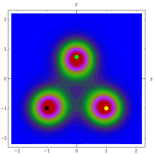
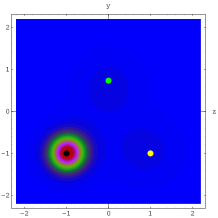
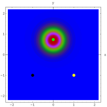
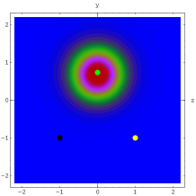
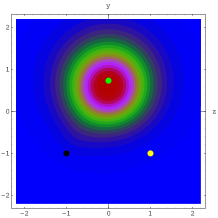
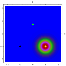
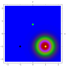
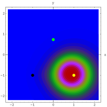
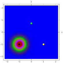
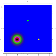
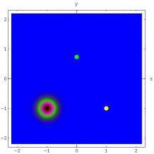
Figure 1: Contour plots of the periodic zero-mode densities in the $x=t=0$ plane for gauge group SU(3). The three columns display, from left to right, the zero-modes corresponding to monopole masses: $m_{1}=m_{2}=m_{3}=2\pi/3$; $m_{1}=m_{2}=\pi/2$, $m_{3}=\pi$; and $m_{1}=m_{2}=\pi/3$, $m_{3}=4\pi/3$. The top row displays the supersymmetric zero-modes and the lower three the non-supersymmetric modes, i.e. $\delta A_{\mu}^{(a)}$ as in Eq. (112), with, from top to bottom, $a=1,2,3$. Monopoles are localised on the vertices of an equilateral triangle of side 2, on the $x=t=0$ plane. The small filled circles indicate the monopole positions, starting from the top monopole in each plot and in clockwise sense: $\vec{X}^{1}$-green, $\vec{X}^{2}$-yellow, $\vec{X}^{3}$-black.

them carries a CP-pair of adjoint zero-modes given in this limit by the solutions parametrised by $\Psi^{(a)}$.

In the opposite limit in which $||\Delta\vec{X}^{a}||<<1,\,\forall a$, the caloron becomes an ordinary BPST instanton and the action density recovers spherical symmetry. For the equal mass case and with monopoles located on the vertices of an equilateral triangle, the symmetry properties allow us to obtain three orthogonal modes, given by the supersymmetric mode and two other linear combinations. The latter are obtained in terms of the following linear combinations of the Nahm data

$$\hat{\Psi}^{(1)}_{11}+\hat{\Psi}^{(2)}_{11}\,e^{-{2\over 3}\pi\sigma_{3}}+\hat{\Psi}^{(3)}_{11}\,e^{\,{2\over 3}\pi\sigma_{3}}\,,$$

$$\hat{\Psi}^{(1)}_{11}+\hat{\Psi}^{(2)}_{11}\,e^{\,{2\over 3}\pi\sigma_{3}}+\hat{\Psi}^{(3)}_{11}\,e^{-{2\over 3}\pi\sigma_{3}}\,,$$

with analogous combinations for the $\delta\tilde{q}^{\dagger}$ terms. The resulting density profiles, for an equilateral triangle of side 0.1, are presented in figure 2.

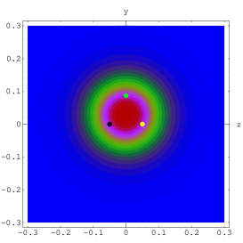
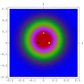
Figure 2: Contour plots of the periodic zero-mode densities at the $t=x=0$ plane for gauge group SU(3) and the equal mass case. The zero-modes have been constructed from orthogonal combinations of the $\Psi^{(a)}$ described in Eq. 7.3.1. The plot on the left corresponds to the supersymmetric mode, the ones on the right display the other two orthogonal modes. Monopoles are localised on the vertices of an equilateral triangle of side 0.1, on the $x=t=0$ plane. The small filled circles indicate the monopole positions, starting from the top monopole in each plot and in clockwise sense: $\vec{X}^{1}$-green, $\vec{X}^{2}$-yellow, $\vec{X}^{3}$-black.

Figure 3 displays the periodic zero-modes for gauge group SU(4) and for equal mass monopoles arranged on the vertices of a square of side 2. Again each non-supersymmetric CP-pair of zero-modes has support on a single constituent monopole. The limit of small separation reproduces again the situation for the BPST instanton.

7.3.2 Anti-periodic zero-modes

In this subsection we will focus on describing a few representative examples of anti-periodic zero-modes for SU(3) and SU(4). We have already discussed in section 6.2 that one has to distinguish two main cases depending on the invertibility of $\mathbf{I}-W_{1}^{\star}W_{1}$. We will only focus on the generic situation which correspond to the invertible case. This covers all the possible cases for SU(3) although not for SU(4).

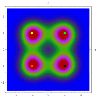
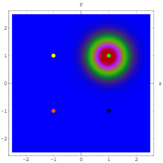
Figure 3: Contour plots of the supersymmetric (left) and non-supersymmetric (right) periodic zero-mode densities on the $x=t=0$ plane for gauge group SU(4) and the equal mass case. We only show one of the non-supersymmetric zero-modes, $\Psi^{(1)}$. The rest look alike but rotated by 90, 180 and 270 degrees along the $x$ symmetry axis. Monopoles are localised on the vertices of a square of side 2, on the $x=t=0$ plane. The small filled circles indicate the monopole positions, starting from the top-right monopole in each plot and in clockwise sense: $\vec{X}^{1}$-green, $\vec{X}^{2}$-black, $\vec{X}^{3}$-red, $\vec{X}^{4}$-yellow.

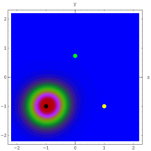
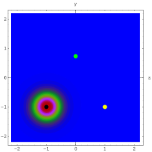
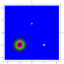
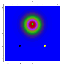
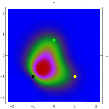
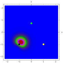
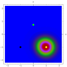
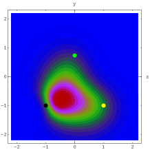
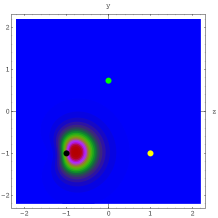
Figure 4: Contour plots of the anti-periodic zero-mode densities on the $x=t=0$ plane for gauge group SU(3). The three columns display, from left to right, the zero-modes corresponding to monopole masses: $m_{1}=m_{2}=m_{3}=2\pi/3$; $m_{1}=m_{2}=\pi/2$, $m_{3}=\pi$; and $m_{1}=m_{2}=\pi/3$, $m_{3}=4\pi/3$. The three rows display the modes corresponding to $\delta A_{\mu}^{(\bar{a})}$ as in Eqs. (126)-(129), with, from top to bottom, $a=1,2,3$. Monopoles are localised on the vertices of an equilateral triangle of side 2, on the $x=t=0$ plane. The small filled circles indicate the monopole positions, starting from the top monopole in each plots and in clockwise sense: $\vec{X}^{1}$-green, $\vec{X}^{2}$-yellow, $\vec{X}^{3}$-black.

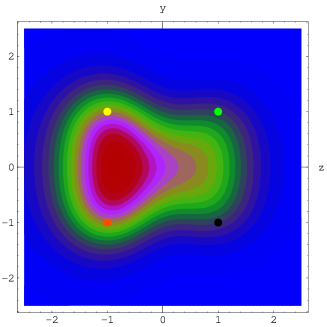
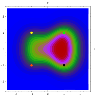
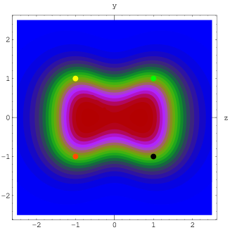
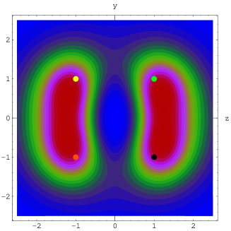
Figure 5: Contour plots of the anti-periodic zero-mode densities on the $x=t=0$ plane for SU(4) and the equal mass case. The relative positions of the monopoles are such that $\Delta\vec{X}^{2}=-\Delta\vec{X}^{4}=-2\hat{k}$. The upper plots display $\Psi^{(\bar{1})}$ (left) and $\Psi^{(\bar{3})}$ (right). The lower plots display the linear combinations $\Psi^{(\bar{1})}-\Psi^{(\bar{3})}$ (left) and $\Psi^{(\bar{1})}+\Psi^{(\bar{3})}$ (right). The remaining modes can be obtained by rotating each of these plots by 90 degrees. Monopoles are localised on the vertices of a square of side 2, on the $x=t=0$ plane. The small filled circles indicate the monopole positions, starting from the top-right monopole in each plot and in clockwise sense: $\vec{X}^{1}$-green, $\vec{X}^{2}$-black, $\vec{X}^{3}$-red, $\vec{X}^{4}$-yellow.

Let us start with the SU(3) case for which the three CP-pairs of solutions, i.e. $\Psi^{(\bar{a})}\equiv\delta A_{\mu}^{(\bar{a})}\sigma_{\mu}$, are given by Eqs. (126)-(129). The first thing that singles out anti-periodic as compared to periodic zero-modes is their localisation with respect to the constituent monopole positions. For well separated monopoles the $\Psi^{(\bar{a})}$ CP-pair of zero-modes has support on the monopole attached to the interval $[Z_{b-1},Z_{b}]$ containing $Z_{\bar{a}}=Z_{a}+\frac{1}{2}$. This gives rise to different possibilities depending on the monopole masses. Fig. 4 displays three characteristic cases corresponding to: $m_{1}=m_{2}=m_{3}=2\pi/3$; $m_{1}=m_{2}=\pi/2$, $m_{3}=\pi$; and $m_{1}=m_{2}=\pi/3$, $m_{3}=4\pi/3$. The first one is analogous to the periodic case (Fig. 1) in that each monopole supports one CP-pair of zero-modes. This changes, however, when one of the monopole masses exceeds $\pi$. In that case the more massive monopole attracts the full set of anti-periodic zero-modes and the rest support none. The intermediate case is a limit between the two situations in which two of the zero-modes become delocalised . These results match the predictions of the index theorem for SU(N) self-dual configurations on $R^{3}\times S^{1}$. We will make here a brief interlude, following Ref. [46], to show that this is indeed the case. We will not give the general formula for the index but we will directly analyse the case for SU(3), relevant for the discussion of Figs. 1 and 4. The reader is referred to Ref. [46] for the general treatment.

The index in the adjoint representation can be written in terms of the topological charge $Q$, the eigenvalues of the holonomy $Z_{a}$ (equivalently the monopole masses) and the magnetic charges $(M_{1},\cdots,M_{N-1})$. The latter are derived from the asymptotic behaviour of the magnetic field at spatial infinity, i.e.

$$\vec{B}(|\vec{x}|\rightarrow\infty)={\vec{x}\over|\vec{x}|^{3}}\,{\rm diag}(n_{1}-n_{N},n_{2}-n_{1},\cdots,n_{N}-n_{N-1})\,,$$ (151)

with magnetic charges given by $M_{i}=n_{i}-n_{N}$. Note that one can fit both calorons and BPS monopoles into this description. For the latter, there are N elementary types of monopoles obtained by setting $n_{i}=1$, with $n_{j\neq i}=0$ and $i=1,\cdots,N$. The monopole that corresponds to taking $i=N$ is usually called the Kaluza-Klein monopole and has magnetic charges $(-1,\cdots,-1)$. Calorons with topological charge $Q=1$ have zero magnetic charge and are obtained by setting all $n_{i}$ equal to one, reproducing therefore the picture of the caloron as a composite of $N$ BPS monopoles.

In terms of the $n_{i}$ and the monopole masses the index in the adjoint representation of SU(3), giving the number of periodic zero-modes, is [46]:

$$I_{\rm adj}(Q,n_{1},n_{2},n_{3})=2NQ\,n_{3}-\sum_{i=1}^{3}n_{i}\,\,\Big{(}2\,[-v_{i}]-2\,[v_{i}]-\sum_{i\neq j}([-v_{j}]-[v_{j}])\Big{)}\,$$ (152)

where $v_{i}=m_{i}/2\pi$, for $i=1,2$, $v_{3}=m_{3}/2\pi-1$, and $[v]\equiv{\rm max}\{n\in{\cal Z}\,|\,n\leq v\}$. Note that the Kaluza-Klein monopole is peculiar in that it receives a contribution from the topological charge term. It is easy to check from the formula that, for monopole masses smaller than $2\pi$ and $Q=1$, each monopole supports 2 periodic zero-modes in agreement with the index theorem by Callias. The formula also gives a correct counting of the number of periodic zero-modes for the $Q=1$ caloron, i.e. 2N. To compute the number of anti-periodic zero-modes we have to resort again to the replica trick. After replicating once in time we obtain that $Q\rightarrow 2Q$ and $v_{i}\rightarrow 2v_{i}$. Accordingly the number of zero-modes for the replicated caloron is $4N$, out of which $2N$ are periodic and $2N$ anti-periodic on the original torus. In what refers to monopoles, it is easy to check that the formula for the index in the replicated torus gives:

• If $m_{1}=m_{2}=m_{3}=2\pi/3$, then: $I_{\rm adj}^{R}(Q=2,n_{1},n_{2},n_{3})=4n_{1}+4n_{2}+(4N-8)n_{3}$. Each monopole supports 4 periodic zero-modes in the replicated torus. This implies two periodic plus two anti-periodic zero-modes in the original configuration as observed in the corresponding plots of Figs. 1 and 4.

• If $m_{1}=m_{2}=\pi/3$, $m_{3}=4\pi/3$, then: $I_{\rm adj}^{R}(Q=2,n_{1},n_{2},n_{3})=2n_{1}+2n_{2}+(4N-4)\,n_{3}$. Monopoles 1 and 2 have only two zero-modes in the replicated torus, while the more massive monopole, attached to $n_{3}$, has 8 zero-modes. Out of those 2 for each monopole correspond to periodic zero-modes of the original configuration. We obtain therefore the result advanced in Figs. 1 and 4: monopoles 1 and 2 support no anti-periodic zero-modes, while monopole 3 carries 6 anti-periodic zero-modes.

More general situations can also be analysed using the expression for the index given in Eq. (152).

We proceed now to present results for the gauge group SU(4). We will restrict the discussion to the case of equal mass monopoles localised on the vertices of a square. Given that the monopole relative positions are coplanar this admits special solutions as the ones discussed in section 6.2. However, we will only consider the case having $\Delta\vec{X}^{2}=-\Delta\vec{X}^{4}=-2\hat{k}$, which belongs to the generic situation in which $\mathbf{I}-W_{1}^{\star}W_{1}$ is invertible. Thus, the zero-modes are given by Eqs. (126)-(129). The alternative choice having $\Delta\vec{X}^{2}=\Delta\vec{X}^{4}=-2\hat{k}$, gives rise to $W_{1}^{\star}W_{1}=\mathbf{I}$. The solutions can be obtained by the construction following Eqs. (132), (133), but will not be presented here.

Figure 5 displays the invertible case with monopoles localised on the vertices of a square of side 2. The fact that zero-modes are not attached to a single BPS monopole is related to a singularity of the equal mass case for SU(4). It happens that every $Z_{\bar{a}}$ coincides with one of the eigenvalues of the holonomy ($Z_{b}$ for some $b$). Consequently it lies between two monopole intervals and the zero-mode density spreads among both. The $a=1$ case for instance has the singularity at $Z_{\bar{1}}=Z_{3}$, therefore the density profile should be attached to monopoles 3 and 4 and aligned with the 3-4 relative position: $\Delta\vec{X}^{4}=2\hat{k}$. The upper-left plot of Fig. 5 shows that this is indeed the case. Note in addition that the anti-parallelism of $\Delta\vec{X}^{2}$ and $\Delta\vec{X}^{4}$ corresponds to the condition for the existence of spurious solutions with modified periodicity described at the end of section 6.1. According to the discussion presented there whenever this condition holds it should be possible to find a pair of zero-modes for which $\hat{\Psi}_{11}=0$ and only the term in $\delta\tilde{q}$ survives. As already discussed, for equal mass monopoles these spurious solutions do give rise to anti-periodic zero-modes. Indeed, two such solutions can be obtained from the linear combinations $\Psi^{(\bar{2})}+\Psi^{(\bar{4})}$ and $\Psi^{(\bar{1})}+\Psi^{(\bar{3})}$. The latter and the alternative combination $\Psi^{(\bar{1})}-\Psi^{(\bar{3})}$ are displayed in Fig. 5.

8 Summary and Outlook

In this paper we have addressed the analytical construction of adjoint zero-modes of the Dirac equation in the background field of SU(N) $Q=1$ calorons, thus extending our previous SU(2) results ([29]-[30]). We have covered both periodic and anti-periodic boundary conditions in time. The latter is useful for the semi-classical study of ${\cal N}=1$ SUSY Yang-Mills at finite temperature and the longstanding issues of Supersymmetry breaking. In this paper we have made an effort to make a complete study of the problem of adjoint zero-modes in SU(N) Yang-Mills theory, presenting general formulas and derivations for the ADHM construction, the Nahm transform on the torus, and, finally, for the caloron case. Thus, we hope this paper could serve as a useful reference for researchers interested in gluino zero-modes.

Although the formulas for SU(N) contain those for the SU(2) case, it is found out that the latter case is quite exceptional in several aspects, so that the generalisation is far from being trivial. Ultimately, given the generality of our formulas, we hope that they will be instrumental in addressing several open issues, including theoretical problems about higher charge calorons, the finite temperature behaviour of SUSY Yang-Mills theory, which the authors intend to address themselves in future publications, and other applications of adjoint zero-modes mentioned in the Introduction of this paper.

Appendix A Appendix.

In this appendix we will collect different formulas and calculations of a more technical type needed to complete the analytical computations of zero-modes described in the text. We will start by generalising the calculation of $u$ and $\omega$ for SU(N) calorons.

A.1 Computation of $\omega$ and $u$

In this subsection we derive explicit formulas for the basic ADHM quantities $\omega$ and $u$ in terms of our Nahm data. Here we will follow the same procedure given in Ref. [29] for SU(2). Most of our formulas are generalised in a simple way, so we will be very sketchy in the derivation and invite the readers to consult that reference.

All interesting functions belong to the space of linear combinations of the following $2N$ functions:

$$\Psi^{\pm}_{a}(z)\equiv\Psi^{(\pm)}(z-Z_{a}^{M},x-X^{a},\frac{m_{a}}{4\pi})\,,$$ (153)

where $m_{a}$ and $X^{a}$ are the mass and position of the a-th constituent monopole, $Z^{M}_{a}$ are the midpoints of the intervals in $z$, $Z_{a}^{M}=(Z_{a}+Z_{a-1})/2$, $x$ is the space-time coordinate and

$$\Psi^{(+)}(z,x,\delta)=\chi(-\delta,\delta)\,e^{i2\pi\bar{x}z}$$ (154)

$$\Psi^{(-)}(z,x,\delta)=\chi(-\delta,\delta)\,e^{i2\pi\hat{x}z}$$ (155)

Using the form of the operator $\widetilde{M}\equiv\widetilde{A}-\hat{x}\,I\!\!I_{Q}$, see Eq. (69), and the equations fulfilled by the functions $u$ and $\omega$, i.e. Eqs. (45)-(48), it is easy to deduce that they can be expanded as:

$$u(z) = \sum_{a}u_{a}(z)=\sum_{a}(\Psi_{a}^{+}(z)A_{a})$$ (156)

$$\omega(z) = \sum_{a}\omega_{a}(z)=\sum_{a}(\Psi_{a}^{+}(z)D_{a}^{(+)}+\Psi_{a}^{-}(z)D_{a}^{(-)})$$ (157)

$$\hat{\partial}\omega = \sum_{a}(4\pi i(z-Z^{M}_{a})\Psi_{a}^{+}(z)D_{a}^{(+)}+\Psi_{a}^{+}(z)S_{a}^{(+)}+\Psi_{a}^{-}(z)S_{a}^{(-)})$$ (158)

where the coefficients ($A_{a}$, $D_{a}^{(\pm)}$, $S_{a}^{(\pm)}$) are $2\times N$ matrix functions of space-time $x$. These can be determined by matching the value of the functions at the edges of the intervals to satisfy the delta function part of the equations. For that we would need to introduce the $2\times 2$ matrix $E^{\prime}$ defined as:

$$E^{\prime\epsilon^{\prime}\epsilon}_{a}=\Psi_{a}^{\epsilon}(z=Z^{M}_{a}+\epsilon^{\prime}\frac{m_{a}}{4\pi})$$ (159)

where $\epsilon$ and $\epsilon^{\prime}$ take the values $\pm 1$. The inverse matrix is given by

$$E_{a}^{\prime-1}=\frac{g(m_{a}r_{a})\hat{n}_{a}}{2m_{a}r_{a}}\times E_{a}^{\dagger}$$ (160)

where $E_{a}$ is a new matrix. The symbol $\hat{n}_{a}$ stands for a hermitian unitary traceless matrix defined through the decomposition

$$(\vec{x}-\vec{X}^{a})\vec{\tau}=r_{a}\hat{n}_{a}$$ (161)

where $r_{a}$ is the distance to the corresponding constituent monopole. The expressions also contain the function $g$:

$$g(u)=u/\sinh(u)$$ (162)

evaluated at the product of the mass and the distance.

The first step in the determination of the coefficients $D^{(\pm)}_{a}$ and $S_{a}^{(\pm)}$ will be to express them in terms of the values of $\omega$ at the points separating the different intervals: $\omega(Z_{a})\equiv{\cal W}_{a}$. Imposing the continuity in $z$ of the function $\omega$ we obtain:

$${\cal W}_{a} = \sum_{\epsilon}E^{\prime+\epsilon}_{a}D_{a}^{(\epsilon)}=\sum_{\epsilon}E^{\prime-\epsilon}_{a+1}D_{a+1}^{(\epsilon)}$$ (163)

$$\hat{\partial}{\cal W}_{a} = im_{a}E^{\prime++}_{a}D_{a}^{(+)}+E^{\prime+\epsilon}_{a}S_{a}^{(\epsilon)}=-im_{a+1}E^{\prime-+}_{a+1}D_{a+1}^{(+)}+E^{\prime-\epsilon}_{a+1}S_{a+1}^{(\epsilon)}$$ (164)

These equations can be rewritten as a vector equation allowing to solve for $D_{a}^{(\pm)}$ in terms of ${\cal W}_{a}$ and ${\cal W}_{a-1}$. Using our previous definitions of the matrices $E_{a}$ and $E^{\prime}_{a}$ we can write:

$$D_{a}^{(\epsilon)} = \frac{\hat{n}_{a}g(m_{a}r_{a})}{2m_{a}r_{a}}(E_{a}^{\dagger})^{\epsilon\epsilon^{\prime}}{\cal W}_{a+(\epsilon^{\prime}-1)/2}$$ (165)

$$S_{a}^{(\epsilon)} = \frac{\hat{n}_{a}g(m_{a}r_{a})}{2m_{a}r_{a}}(E_{a}^{\dagger})^{\epsilon\epsilon^{\prime}}\hat{\partial}{\cal W}_{a+(\epsilon^{\prime}-1)/2}+\frac{ig^{2}(m_{a}r_{a})}{2m_{a}r_{a}^{2}}\widetilde{E}^{\epsilon}(E_{a}^{\dagger})^{+\epsilon^{\prime}}{\cal W}_{a+(\epsilon^{\prime}-1)/2}$$ (166)

where $\widetilde{E}^{+}=\cosh(m_{a}r_{a})$ and $\widetilde{E}^{-}=-1$. The coefficient $A_{a}$ appearing in the expansion of $u$ can be related to $D_{a}^{(+)}$ by the equation $\widetilde{M}\omega=uF^{-1}$. Hence, we get

$$A_{a}=2ir_{a}\hat{n}_{a}D_{a}^{(+)}F$$ (167)

Notice that the functions $u_{a}$ and $\omega_{a}$ can be regarded as the contribution of the a-th constituent monopole to the function $u$ and $\omega$, since they only depend on the distance $r_{a}$ and the mass $m_{a}$ of the corresponding monopole. Nonetheless, the mixing and interaction among the constituent monopoles is hidden in the expression of ${\cal W}_{a}$, which we will now derive. The main equation satisfied by ${\cal W}_{a}$ comes from the equation:

$$q=\widetilde{M}^{\dagger}u$$ (168)

leading to

$$\zeta_{\alpha}^{a}P_{a}=\frac{-1}{2\pi i}(E_{a}^{\prime++}A_{a}-E_{a+1}^{\prime-+}A_{a+1})$$ (169)

where $P_{a}$ is an N-vector with components $\delta_{ai}$. To write the previous equation in a more compact form we arrange the right hand side into an N-component column vector of $2\times N$ matrices. The unknown ${\cal W}_{a}$ are also arranged as a column vector of the same kind. Finally, we introduce the N-component column vectors of quaternions $e_{a}$ and $\widetilde{e}_{a}$ whose components are $2\times 2$ matrices and such that the only non-zero components are the rows $a-1$ and $a$, given by

$$e^{a-1}_{a}= E_{a}^{\prime-+}\ ;\quad e^{a}_{a}=-E_{a}^{\prime++}$$ (170)

$$\widetilde{e}^{a-1}_{a}= - E_{a}^{\prime--}\ ;\quad\widetilde{e}^{a}_{a}=\ \ E_{a}^{\prime+-}$$ (171)

Then the previous equations can be re-written as follows:

$$\zeta=\sum_{a}\frac{g(m_{a}r_{a})}{2\pi m_{a}}e_{a}e_{a}^{\dagger}{\cal W}F$$ (172)

The projector $e_{a}e_{a}^{\dagger}$ is an $N\times N$ matrix of quaternions whose only non-zero components correspond to the $a-1$ and $a$ rows and columns. Restricting to this non-zero $2\times 2$ matrix we have

$$\frac{g(m_{a}r_{a})}{2\pi m_{a}}e_{a}e_{a}^{\dagger}\big{|}_{\mbox{\rm\tiny restricted}}=\frac{g(m_{a}r_{a})}{2\pi m_{a}}\pmatrix{\cosh(m_{a}r_{a})&-e^{-im_{a}x_{0}}\cr-e^{im_{a}x_{0}}&\cosh(m_{a}r_{a})}+\frac{1}{2\pi}\vec{\tau}\pmatrix{\vec{x}-\vec{X}^{a}&0\cr 0&-\vec{x}+\vec{X}^{a}}$$ (173)

The first term on the right-hand side can be completed (with zeroes) to an $N\times N$ complex matrix that we will call $U_{a}$. The second piece when summed over “a” can be rewritten in terms of the projector $\zeta\zeta^{\dagger}$. In this way Eq. (172) can be rewritten as

$$\zeta=V^{-1}{\cal W}F-\zeta\zeta^{\dagger}{\cal W}F$$ (174)

where

$$V^{-1}=\sum_{a}U_{a}+\frac{1}{2\pi}\mbox{diag}(||\vec{X}^{a+1}-\vec{X}^{a}||)$$ (175)

Using the definition of $F$

$$F^{-1}=\mathbf{I}-\zeta^{\dagger}{\cal W}$$ (176)

we finally arrive to

$$\zeta=V^{-1}{\cal W}$$ (177)

whose solution is

$${\cal W}=V\zeta$$ (178)

The matrix $V$ is an $N\times N$ complex hermitian matrix. The elements of $F^{-1}$ can be obtained in terms of this matrix

$$(F^{-1})_{ab}=\delta_{ab}-V_{ab}\zeta^{\dagger}_{a}\zeta_{b}$$ (179)

A.2 Field strength and periodic zero-modes

In section 6.1 we expressed the zero-modes in terms of 2 sets of functions $E_{\mu}^{(a)}$ and $\tilde{E}_{\mu}^{(a)}$ where the label $a$ runs from 1 to N. With the aid of the formulas of the previous subsection one can compute these functions.

Let us start with the computation of $E_{\mu}^{(a)}$ defined in Eq. (111). Using the definitions of $u_{a}$ and $\omega_{a}$ of the previous subsection it can be re-expressed as

$$E_{\mu}^{(a)}=\frac{i}{2}F^{-1/2}\int dz\,u_{a}^{\dagger}(z)\bar{\sigma}_{\alpha}\hat{\partial}\omega_{a}(z)F^{1/2}+{\rm h.c.}$$ (180)

To obtain the corresponding expression one must perform the integration in z. Notice that all the $z$ dependence of $u_{a}$ and $\omega_{a}$ enters through the $\Psi_{a}^{\pm}$ functions. Their integrals can be performed analytically leading to the expression

$$I^{\pm}_{\alpha}=\int dz\Psi_{b}^{+\dagger}\bar{\sigma}_{\alpha}\Psi_{a}^{\pm}=\delta_{ab}\frac{m_{a}}{2\pi}({\cal P}^{a\,\alpha}_{\pm}\frac{1}{g(m_{a}r_{a})}+{\cal P}^{a\,\alpha}_{\mp})\,,$$ (181)

One needs in addition the following integral

$$\widetilde{I}_{\alpha}=4\pi i\int dz(z-Z_{M}^{a})\Psi_{b}^{+\dagger}\bar{\sigma}_{\alpha}\Psi_{a}^{+}=\delta_{ab}\frac{m_{a}^{2}}{2\pi}\left(\frac{g^{\prime}(m_{a}r_{a})}{g^{2}(m_{a}r_{a})}\right){\cal P}^{a\,\alpha}_{+}(i\hat{n}_{a})\,,$$ (182)

In the final expressions we have introduced the quaternions

$${\cal P}^{a\,\alpha}_{\pm}=\frac{1}{2}(\bar{\sigma}^{\alpha}\pm\hat{n}_{a}\bar{\sigma}^{\alpha}\hat{n}_{a})\,,$$ (183)

where $\hat{n}_{a}$ and $g(u)$ have been defined in Eqs. (161) and (162).

Using the previous formulas and those of the first subsection of the appendix we arrive at

$$E_{\mu}^{(a)}=\frac{i}{2}F^{1/2}{\cal W}^{\dagger}{\cal L}_{a\alpha}{\cal W}F^{1/2}+\frac{i}{2}F^{1/2}{\cal W}^{\dagger}\widetilde{{\cal L}}_{a}\bar{\sigma}_{\alpha}\hat{\partial}{\cal W}F^{1/2}+{\rm h.c.}$$ (184)

where

$${\cal L}_{a\alpha}=-\frac{im_{a}g(m_{a}r_{a})}{2\pi}e_{a}\left(-i\frac{g^{2}(m_{a}r_{a})-1}{2m_{a}^{2}r_{a}^{2}}{\cal P}^{a\,\alpha}_{+}-i\frac{g^{\prime}(m_{a}r_{a})}{2m_{a}r_{a}}{\cal P}^{a\,\alpha}_{-}\right)e_{a}^{\dagger}$$ (185)

and

$$\widetilde{{\cal L}}_{a}=\frac{-ig(m_{a}r_{a})}{4\pi m_{a}r_{a}}e_{a}\hat{n}_{a}\left(g(m_{a}r_{a})\widetilde{e}_{a}^{\dagger}+e_{a}^{\dagger}\right)$$ (186)

Using the relation between the quantity inside parenthesis in Eq. (185) with the gauge field of a SU(2) BPS monopole we can write this first term as

$$\sum_{a}E^{\rm BPS}_{i}(x-X^{a};m_{a})I_{i}^{a}$$ (187)

where we have introduced the $N\times N$ hermitian matrices $I_{i}^{a}$ given by

$$I_{i}^{a}=\frac{g(m_{a}r_{a})}{2\pi m_{a}}F^{1/2}{\cal W}^{\dagger}e_{a}\tau_{i}e_{a}^{\dagger}{\cal W}F^{1/2}$$ (188)

they provide an embedding of the SU(2) group in SU(N).

In this way all our formulas are expressed in terms of the values of $\omega(Z_{b})={\cal W}_{b}$. The latter can be expressed in terms of the matrix $V$ defined in the first subsection of the appendix. The same quantities also appear in the expression of $\tilde{E}_{\mu}^{(a)}$, as shown in Eq. (113).

Notice that the electric field strength is a particular case of the previous formula, since $E_{i}=\sum_{a}E^{(a)}_{i}$.

A.3 Anti-periodic zero-mode formulas

The corresponding expressions for the anti-periodic zero-modes are considerably more involved, although again the integrals appearing in Eq. (129) can also be performed analytically. The main difference with respect to the periodic case is that in the latter each mode in the basis depends on a single region $(Z_{a-1},Z_{a})$ associated to a given constituent monopole. The formula only depends on the remaining monopole positions through the matrix $F$. In the anti-periodic case, the expressions involve pairs of monopoles, namely those pairs such that

$$(Z_{a-1},Z_{a})\cap(Z_{b-1}+{1\over 2},Z_{b}+{1\over 2})\neq\emptyset$$ (189)

The condition can be easily implemented if we introduce $\chi_{\bar{b}}$ as the characteristic function of the interval $(Z_{b-1}+{1\over 2},Z_{b}+{1\over 2})$. Then, one can rewrite

$$\hat{\Psi}^{a}_{12}(z)\equiv\sum_{b\,c}\hat{\Psi}^{abc}_{12}(z)=\sum_{b\,c}\chi_{b}\chi_{\bar{c}}\exp\{2\pi\tau_{i}(X_{i}^{b}-X_{i}^{c})z\}\kappa_{abc}$$ (190)

where the coefficient matrices $\kappa_{abc}$ follow from simple linear relations in terms of ${\cal U}_{AB}$ and $\kappa_{\pm}^{A}$. Notice then that, due to the characteristic functions, the integrals appearing in the expression of the anti-periodic zero-modes Eq. (129) only involve integrals of $\hat{\Psi}^{abc}_{12}(z)$ with $u_{b}$ and $\omega_{c}$. Using appropriate matrix projections, these integrals reduce to those of ordinary exponentials. The details are somewhat cumbersome and we will skip them here.

References

- [1] N. M. Davies, T. J. Hollowood, V. V. Khoze and M. P. Mattis, Nucl. Phys. B 559 (1999) 123 [arXiv:hep-th/9905015]. N. M. Davies, T. J. Hollowood and V. V. Khoze, J. Math. Phys. 44 (2003) 3640 [arXiv:hep-th/0006011].
- [2] P. Kovtun, M. Unsal and L. G. Yaffe, JHEP 0706 (2007) 019 [arXiv:hep-th/0702021].
- [3] M. Unsal and L. G. Yaffe, Phys. Rev. D 78 (2008) 065035 [arXiv:0803.0344 [hep-th]].
- [4] M. Unsal, Phys. Rev. Lett. 100 (2008) 032005 [arXiv:0708.1772 [hep-th]].
- [5] J. C. Myers and M. C. Ogilvie, “Phase diagrams of SU(N) gauge theories with fermions in various representations,” arXiv:0903.4638 [hep-th].
- [6] G. Cossu and M. D’Elia, “Finite size phase transitions in QCD with adjoint fermions,” arXiv:0904.1353 [hep-lat].
- [7] T. Eguchi and H. Kawai, Phys. Rev. Lett. 48 (1982) 1063. A. González-Arroyo and M. Okawa, Phys. Lett. B 120 (1983) 174; Phys. Rev. D 27 (1983) 2397. G. Bhanot, U. M. Heller and H. Neuberger, Phys. Lett. B 113 (1982) 47.
- [8] T. C. Kraan and P. van Baal, Phys. Lett. B 428 (1998) 268 [arXiv:hep-th/9802049]. Nucl. Phys. B 533 (1998) 627 [arXiv:hep-th/9805168].
- [9] T. C. Kraan and P. van Baal, Phys. Lett. B 435 (1998) 389 [arXiv:hep-th/9806034].
- [10] K. M. Lee, Phys. Lett. B 426 (1998) 323 [arXiv:hep-th/9802012].
- [11] K. M. Lee and C. h. Lu, Phys. Rev. D 58, 025011 (1998) [arXiv:hep-th/9802108].
- [12] B. J. Harrington and H. K. Shepard, Phys. Rev. D 17, 2122 (1978). Phys. Rev. D 18 (1978) 2990.
- [13] A. A. Belavin, V. A. Fateev, A. S. Schwarz and Y. S. Tyupkin, Phys. Lett. B 83 (1979) 317.
- [14] C. G. . Callan, R. F. Dashen and D. J. Gross, Phys. Rev. D 17 (1978) 2717.
- [15] M. García Perez, A. González-Arroyo and P. Martínez, Nucl. Phys. Proc. Suppl. 34 (1994) 228 [arXiv:hep-lat/9312066]. A. González-Arroyo and P. Martínez, Nucl. Phys. B 459 (1996) 337 [arXiv:hep-lat/9507001]. A. González-Arroyo, P. Martínez and A. Montero, Phys. Lett. B 359 (1995) 159 [arXiv:hep-lat/9507006]. A. González-Arroyo and A. Montero, Phys. Lett. B 387 (1996) 823 [arXiv:hep-th/9604017].
- [16] D. J. Gross, R. D. Pisarski and L. G. Yaffe, Rev. Mod. Phys. 53 (1981) 43.
- [17] D. Diakonov and V. Petrov, Phys. Rev. D 76 (2007) 056001 [arXiv:0704.3181 [hep-th]]. D. Diakonov, N. Gromov, V. Petrov and S. Slizovskiy, Phys. Rev. D 70 (2004) 036003 [arXiv:hep-th/0404042]. D. Diakonov, Acta Phys. Polon. B 39 (2008) 3365 [arXiv:0807.0902 [hep-th]]. P. Gerhold, E. M. Ilgenfritz and M. Muller-Preussker, Nucl. Phys. B 760 (2007) 1 [arXiv:hep-ph/0607315].
- [18] C. Gattringer, Phys. Rev. D 67 (2003) 034507 [arXiv:hep-lat/0210001]. C. Gattringer and S. Schaefer, Nucl. Phys. B 654 (2003) 30 [arXiv:hep-lat/0212029]. C. Gattringer and R. Pullirsch, Phys. Rev. D 69 (2004) 094510 [arXiv:hep-lat/0402008]. E. M. Ilgenfritz, B. V. Martemyanov, M. Muller-Preussker, S. Shcheredin and A. I. Veselov, Phys. Rev. D 66 (2002) 074503 [arXiv:hep-lat/0206004]. Phys. Rev. D 69 (2004) 114505 [arXiv:hep-lat/0402010]. E. M. Ilgenfritz, B. V. Martemyanov, M. Muller-Preussker and A. I. Veselov, Phys. Rev. D 71 (2005) 034505 [arXiv:hep-lat/0412028]. E. M. Ilgenfritz, M. Muller-Preussker and D. Peschka, Phys. Rev. D 71 (2005) 116003 [arXiv:hep-lat/0503020]. E. M. Ilgenfritz, B. V. Martemyanov, M. Muller-Preussker and A. I. Veselov, Phys. Rev. D 73 (2006) 094509 [arXiv:hep-lat/0602002]. V. G. Bornyakov, E. M. Ilgenfritz, B. V. Martemyanov, S. M. Morozov, M. Muller-Preussker and A. I. Veselov, Phys. Rev. D 76 (2007) 054505 [arXiv:0706.4206 [hep-lat]]. V. G. Bornyakov, E. M. Ilgenfritz, B. V. Martemyanov and M. Muller-Preussker, Phys. Rev. D 79 (2009) 034506 [arXiv:0809.2142 [hep-lat]].
- [19] F. Bruckmann, S. Dinter, E. M. Ilgenfritz, M. Muller-Preussker and M. Wagner, “Cautionary remarks on the moduli space metric for multi-dyon simulations,” arXiv:0903.3075 [hep-ph].
- [20] A. K. Das and M. Kaku, Phys. Rev. D 18 (1978) 4540.
- [21] L. Girardello, M. T. Grisaru and P. Salomonson, Nucl. Phys. B 178 (1981) 331.
- [22] L. Van Hove, Nucl. Phys. B 207 (1982) 15.
- [23] H. Aoyama and D. Boyanovsky, Phys. Rev. D 30 (1984) 1356.
- [24] D. Boyanovsky, Phys. Rev. D 29 (1984) 743.
- [25] H. Matsumoto, M. Nakahara, Y. Nakano and H. Umezawa, Phys. Lett. B 140 (1984) 53; Phys. Rev. D 29 (1984) 2838.
- [26] D. Buchholz and I. Ojima, Nucl. Phys. B 498 (1997) 228 [arXiv:hep-th/9701005].
- [27] M. García Perez, A. González-Arroyo, C. Pena and P. van Baal, Phys. Rev. D 60 (1999) 031901 [arXiv:hep-th/9905016].
- [28] M. N. Chernodub, T. C. Kraan and P. van Baal, Nucl. Phys. Proc. Suppl. 83 (2000) 556 [arXiv:hep-lat/9907001]. F. Bruckmann, D. Nogradi and P. van Baal, Nucl. Phys. B 666 (2003) 197 [arXiv:hep-th/0305063].
- [29] M. García Perez and A. González-Arroyo, JHEP 0611 (2006) 091 [arXiv:hep-th/0609058].
- [30] M. García Perez, A. González-Arroyo and A. Sastre, Phys. Lett. B 668 (2008) 340 [arXiv:0807.2285 [hep-th]].
- [31] A. González-Arroyo and R. Kirchner, JHEP 0601 (2006) 029 [arXiv:hep-lat/0507036].
- [32] M. García Perez, A. González-Arroyo and A. Sastre, PoS LAT2007 (2007) 328 [arXiv:0710.0455 [hep-lat]].
- [33] M. F. Atiyah and I. M. Singer, Annals Math. 87 (1968) 484;
- [34] C. W. Bernard, N. H. Christ, A. H. Guth and E. J. Weinberg, Phys. Rev. D 16 (1977) 2967. A. S. Schwarz, Phys. Lett. B 67 (1977) 172. M. F. Atiyah, N. J. Hitchin and I. M. Singer, Proc. Roy. Soc. Lond. A 362 (1978) 425.
- [35] M. F. Atiyah, N. J. Hitchin, V. G. Drinfeld and Y. I. Manin, Phys. Lett. A 65 (1978) 185.
- [36] E. Corrigan,D.B. Fairlie, S. Templeton and P. Goddard, Nucl. Phys. B 140 (1978) 31. H. Osborn, Nucl. Phys. B140 (1978) 45.
- [37] E. Corrigan, P. Goddard and S. Templeton, Nucl. Phys. B 151 (1979) 93.
- [38] N. H. Christ, E. J. Weinberg and N. K. Stanton, Phys. Rev. D 18 (1978) 2013.
- [39] W. Nahm, Phys. Lett. B 90 (1980) 413; “All Selfdual Multi - Monopoles For Arbitrary Gauge Groups,” CERN-TH-3172 Presented at Int. Summer Inst. on Theoretical Physics, Freiburg, West Germany, Aug 31 - Sep 11, 1981
- [40] P. J. Braam and P. van Baal, Commun. Math. Phys. 122 (1989) 267.
- [41] A. González-Arroyo, Nucl. Phys. B 548 (1999) 626 [arXiv:hep-th/9811041].
- [42] E. Bilgici, F. Bruckmann, C. Gattringer and C. Hagen, Phys. Rev. D 77 (2008) 094007 [arXiv:0801.4051 [hep-lat]].
- [43] E. Bilgici, C. Gattringer, E. M. Ilgenfritz and A. Maas, “Adjoint quarks and fermionic boundary conditions,” arXiv:0904.3450 [hep-lat].
- [44] T. C. Kraan, Commun. Math. Phys. 212 (2000) 503 [arXiv:hep-th/9811179].
- [45] C. Callias, Commun. Math. Phys. 62 (1978) 213.
- [46] T. M. W. Nye and M. A. Singer, “An -Index Theorem for Dirac Operators on ,” arXiv:math/0009144. E. Poppitz and M. Unsal, JHEP 0903 (2009) 027 [arXiv:0812.2085 [hep-th]].