Rossby waves and $\alpha$-effect

Abstract

Rossby waves drifting in the azimuthal direction are a common feature at the onset of thermal convective instability in a rapidly rotating spherical shell. They can also result from the destabilization of a Stewartson shear layer produced by differential rotation as expected in the liquid sodium experiment (DTS) working in Grenoble, France.

A usual way to explain why Rossby waves can participate to the dynamo process goes back to Busse (1975). In his picture, the flow geometry is a cylindrical array of parallel rolls aligned with the rotation axis. The axial flow component (the component parallel to the rotation axis) is (i) maximum in the middle of each roll and changes its sign from one roll to the next. It is produced by the Ekman pumping at the fluid containing shell boundary. The corresponding dynamo mechanism can be explained in terms of an $\alpha$-tensor with non-zero coefficients on the diagonal. It corresponds to the heuristic picture given by Busse (1975).

In rapidly rotating objects like the Earth’s core (or in a fast rotating experiment), Rossby waves occur in the limit of small Ekman number ($\approx 10^{-15}$). In that case, the main source of the axial flow component is not the Ekman pumping but rather the “geometrical slope effect” due to the spherical shape of the fluid containing shell. This implies that the axial flow component is (ii) maximum at the borders of the rolls and not at the centers. If assumed to be stationary, such rolls would lead to zero coefficients on the diagonal of the $\alpha$-tensor, making the dynamo probably less efficient if possible at all. Actually, the rolls are drifting as a wave, and we show that this drift implies non–zero coefficients on the diagonal of the $\alpha$-tensor. These new coefficients are in essence very different from the ones obtained in case (i) and cannot be interpreted in terms of the heuristic picture of Busse (1975). They were interpreted as higher-order effects in Busse (1975). In addition we considered rolls not only drifting but also having an arbitrary radial phase shift as expected in real objects.

1 Introduction

Rossby waves naturally result from thermal convection instabilities in a rapidly rotating shell. Different configurations have been studied depending on whether the fluid lies between two concentric spherical shells or inside a full sphere, and on the type of heating (either differential or internal). At the instability onset, the motion takes the form of rolls aligned with the axis of rotation and localized at the vicinity of a cylinder lying in the bulk of the fluid. These rolls drift usually as a wave in the prograde azimuthal direction. In each roll in addition to the horizontal flow, that is, the flow in a plane perpendicular to the axis of rotation, there is also an axial flow (component parallel to the rotation axis) due to the boundary conditions at the ends of the rolls.

In rapidly rotating objects like the Earth’s core, the Ekman number $E$, defined as the ratio of the viscous to the Coriolis forces, is small ($E\propto 10^{-15}$). Rossby wave as a linear solution of the thermal convection problem in the asymptotic limit of small Ekman number $E\ll 1$, was first proposed by Busse (1970) (see also the contribution by Roberts 1968). After several intermediate improvements (Soward, 1977; Yano, 1992), an exact solution was given by Jones et al. (2000). Since then, the solution has been confirmed numerically by Dormy et al. (2004) (see also Zhang 1991, 1992; Zhang and Jones 1993). These results assume the asymptotic limit $Pr/E\rightarrow\infty$ where $Pr$ is the Prandtl number defined as the ratio of the viscosity to the thermal diffusivity. Additional issues have been addressed, in the asymptotic limit $Pr/E\rightarrow 0$ (Zhang, 1995) and in the general case $0\leq Pr/E<\infty$ (Zhang et al., 2007), including discussions about the nature of Rossby waves versus inertial waves (Busse et al., 2005).

Thermal Rossby waves have been studied also experimentally (Busse and Carrigan 1976; Carrigan and Busse 1983; Cardin and Olson 1994, see also the review paper by Busse 2002 and references therein). Above the onset the flow becomes highly turbulent and the non-linearities may be strong. Though depending in a complex way on the parameters of the problem (Grote and Busse, 2001; Busse, 2002; Morin and Dormy, 2004), it is worth noting that the persistence of the columnar structure of Rossby waves has been observed both experimentally and numerically (Aubert et al., 2003; Cardin and Olson, 1994; Sumita and Olson, 2000).

When the fluid is electrically conducting such Rossby waves, in combination with differential rotation, are expected to produce dynamo action (Kageyama and Sato, 1997). In addition, by processes related to a 2D inverse cascade (Sommeria, 1986; Aubert et al., 2001) or to the presence of a strong toroidal magnetic field (Cardin and Olson, 1995), the number of rolls for a very low Ekman number is expected to be much lower than estimated from the asymptotic theory of the onset of thermal convection. Therefore, though the parameters in numerical simulations or experiments are far from those of the Earth’s outer core, these studies suggest that the existence of Rossby waves in the form of columnar structures of reasonable size may occur and be important in the geodynamo process.

Rossby waves can also be obtained mechanically, instead of thermally, as shown by Hide and Titman (1967) and Busse (1968). More recently Schaeffer and Cardin (2005a) considered a fluid between two concentric spherical shells in fast rotation but with slightly different rotation rates. They found that the destabilization of the Stewartson shear layer at the tangent cylinder leads indeed to Rossby waves. They have shown that such Rossby waves with the strong differential rotation present in the fluid are capable of dynamo action (Schaeffer and Cardin, 2006). This has enforced the interest in building a new experiment in liquid sodium, called DTS (Cardin et al., 2002; Nataf et al., 2006; Schmitt et al., 2008).

In dynamo theory, it is known for long that differential rotation, that is the $\Omega$-effect, can generate a toroidal magnetic field from a poloidal magnetic field (see e.g. Elsasser 1956). The comprehensive picture given by Busse (1975) illustrates how the interaction of Rossby waves with a toroidal magnetic field can generate toroidal electric currents and thus a poloidal magnetic field. Within the mean–field concept this process can be described in terms of an $\alpha$–effect. The overall dynamo mechanism is known as an $\alpha\Omega$-dynamo.

We can show by simple arguments, that the efficiency of the process described by Busse (1975), or the magnitude of the $\alpha$–effect, depends critically on the relative positions of the horizontal and axial components of the flow in each roll. As a first step let us ignore the drift of the rolls. As illustrated in figure 2a, each roll rotates around its axis with a rotation rate changing its sign from one roll to the adjacent ones. We distinguish between the two cases in which the axial flow is maximum either (i) within each roll or (ii) between two adjacent rolls (top row of figure 1). A given large scale azimuthal magnetic field $\overline{\rm\textbf{B}}$ is stretched by the fluid motion leading to a secondary magnetic field b (middle row of figure 1). Then an azimuthal electromotive force $\rm\textbf{u}\times\rm\textbf{b}$ is created (bottom row of figure 1).

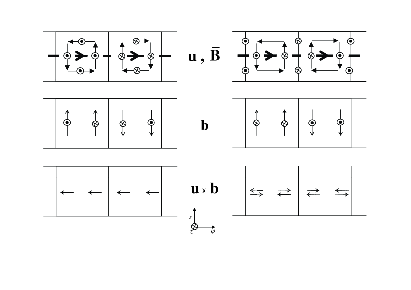
(i)                                                            (ii)

Figure 1: In two adjacent rolls, the fluid velocity u (small arrows and inwards/outwards symbols in first row) acting on a given azimuthal mean magnetic field $\overline{\rm\textbf{B}}$ (thick arrow in top row) results in a secondary magnetic field b (middle row), and so in an electromotive force $\rm\textbf{u}\times\rm\textbf{b}$ (bottom row). The radial, azimuthal and axial directions correspond to $s$, $\varphi$ and $z$. Left column: case (i), for which the axial flow is maximum within each roll. Right column: case (ii), for which the axial flow is maximum between each roll. In case (i) u and b are clearly not parallel or antiparallel, and the azimuthal component of $\rm\textbf{u}\times\rm\textbf{b}$ has the same sign everywhere in the considered points, that is, its azimuthal average is non–zero. By contrast in case (ii) u and b are presumably more or less parallel or antiparallel in the considered points so that $\rm\textbf{u}\times\rm\textbf{b}$ is small. Moreover the azimuthal component of $\rm\textbf{u}\times\rm\textbf{b}$ has different signs in each cell. These aspects suggest that its average vanishes.

For case (i) all local electromotive forces act in the same sense and so generate a global azimuthal electric current. This can be interpreted as an $\alpha$–effect. On the other hand, for case (ii) local electromotive forces with opposite signs occur, implying eventually that there is no global azimuthal electric current, that is, no $\alpha$–effect.

In a rapidly rotating shell with a rigid boundary for which the no–slip condition applies, and relying on the quasi-geostrophic approximation, the axial flow $u_{z}$ in each roll is the sum of two terms. One term is the Ekman pumping, scaling as $E^{1/2}$ and its intensity is maximum within each roll as in case (i). The other term is the geometrical slope effect at the ends of the rolls, scaling as $E^{0}$ and proportional to the radial flow $u_{s}$. It is then of maximum intensity between two adjacent cells as in case (ii). It is argued in Schaeffer and Cardin (2005a) that in rapidly rotating spherical shells like the Earth’s liquid core, the Ekman number is so small that the first term in $u_{z}$ can be neglected compared to the second one. Then in the light of the arguments illustrated in figure 1 (ii) the ability of such a flow to generate an $\alpha$-effect for $E\ll 1$ could appear questionable. Actually in such rapidly rotating systems, stationary convection can not occur. The rolls have to drift as a wave. Then taking this drift into account, we shall demonstrate that even in case (ii) an $\alpha$–effect remains possible. A similar effect is described as an higher-order effect in Busse (1975). However we stress here that this $\alpha$–effect is in essence very different from the one that would be obtained with a flow geometry (i).

Finally, we stress that the $\alpha$-effect, so far understood as the generation of a toroidal mean electromotive force from a toroidal mean magnetic field, and described by only one $\alpha$-coefficient, is in fact a special case of a more general connection between mean electromotive force and mean magnetic field, described by an $\alpha$-tensor. We shall calculate the additional coefficients of this $\alpha$-tensor and give their scaling properties in terms of the flow parameters like the number of rolls, the Rossby wave frequency and the magnetic Reynolds numbers (horizontal and vertical) of the flow. Depending on these parameters these additional coefficients may be dominant compared to the $\alpha$–effect mentioned above and then completely change the overall picture of the possible dynamo mechanism. We shall see that it is all the more true for rolls not only drifting but also having a radial shift as expected for Rossby waves traveling in a spherical shell. In that case the rolls are bent as illustrated in figure 2b.

In section 2 we set the problem, give the basic equations, define the general assumptions and specify the velocity field. In section 3 we derive general analytical expressions for the mean electromotive force with respect to a cylindrical coordinate system. In section 4 we present asymptotic and numerical results for both cases (i) and (ii). Finally, in section 5 we discuss our results.

2 General concept

2.1 Basic equations and assumptions

We consider a body of a homogeneous electrically conducting incompressible fluid, penetrated by a magnetic field B and showing internal motions with a velocity U. The magnetic field B is assumed to be governed by the induction equation

$$\eta{\mbox{\boldmath$\nabla$}}^{2}\rm\textbf{B}+{\mbox{\boldmath$\nabla$}}\times(\rm\textbf{U}\times\rm\textbf{B})-\partial_{t}\rm\textbf{B}={\bf 0}\,,\quad\nabla\cdot\rm\textbf{B}=0,$$ (1d,e)

where $\eta$ is the magnetic diffusivity, considered as constant.

Referring to a cylindrical coordinate system $(s,\varphi,z)$ we define mean fields as in Braginskii’s theory of the nearly axisymmetric dynamo (, 1964a,b) by averaging over $\varphi$. Given a scalar field $F$, the corresponding mean field is denoted by $\overline{F}$. It corresponds to the axisymmetric part of $F$. In the case of vectors or tensors the same definition applies to each component so that, e.g., $\overline{\rm\textbf{B}}=(\overline{B}_{s},\overline{B}_{\varphi},\overline{B}_{z})$.

We split B and U into mean fields, $\overline{\rm\textbf{B}}$ and $\overline{\rm\textbf{U}}$, and deviations b and u from them, that is,

$$\rm\textbf{B}=\overline{\rm\textbf{B}}+\rm\textbf{b}\,,\quad\rm\textbf{U}=\overline{\rm\textbf{U}}+\rm\textbf{u}\,.$$ (2d,e)

From the induction equation (1e,f) we obtain

$$\eta{\mbox{\boldmath$\nabla$}}^{2}\overline{\rm\textbf{B}}+{\mbox{\boldmath$\nabla$}}\times(\overline{\rm\textbf{U}}\times\overline{\rm\textbf{B}})+{\mbox{\boldmath$\nabla$}}\times{\mbox{\boldmath$\cal{E}$}}-\partial_{t}\overline{\rm\textbf{B}}={\bf 0}\,,\quad\nabla\cdot\overline{\rm\textbf{B}}=0,$$ (3d,e)

where

$${\mbox{\boldmath$\cal{E}$}}=\overline{\rm\textbf{u}\times\rm\textbf{b}}$$ (4)

is the mean electromotive force due to u and b.

In view of the generation of a mean magnetic field, two terms of the equation (3e,f) are of particular interest, that with $\overline{\rm\textbf{U}}$ and that with $\cal{E}$. We assume here that the mean velocity $\overline{\rm\textbf{U}}$ corresponds to a rotation only. We further think of a proper specification of the small-scale velocity u so that $\cal{E}$ covers the effect of Rossby waves. For the determination of $\cal{E}$ we assume rigid-body mean rotation, that is we ignore any differential rotation, and adopt a co-rotating frame of reference in which $\overline{\rm\textbf{U}}=0$. According to (4) $\cal{E}$ is determined by u, which we consider as given, and b. Using (1e,f), (2e,f) and (3e,f) we obtain

$$\eta{\mbox{\boldmath$\nabla$}}^{2}\rm\textbf{b}+{\mbox{\boldmath$\nabla$}}\times(\rm\textbf{u}\times\overline{\rm\textbf{B}})+{\mbox{\boldmath$\nabla$}}\times(\rm\textbf{u}\times\rm\textbf{b}-\overline{\rm\textbf{u}\times\rm\textbf{b}})-\partial_{t}\rm\textbf{b}={\bf 0}\,,\quad\nabla\cdot\rm\textbf{b}=0\,.$$ (5d,e)

Clearly this equation determines b if u and $\overline{\rm\textbf{B}}$ are given.

In order to make analytical calculations possible we introduce a quasi-linear approximation (also known as the second-order correlation approximation in mean field theory), that is we neglect the term $|{\mbox{\boldmath$\nabla$}}\times(\rm\textbf{u}\times\rm\textbf{b}-\overline{\rm\textbf{u}\times\rm\textbf{b}})|$ in (5e,f). A sufficient condition for that approximation is

$$\min(R_{m}^{\prime},S_{t})\ll 1$$ (6)

with the magnetic Reynolds number $R_{m}^{\prime}=u_{0}l^{\prime}/\eta$, and the Strouhal number $S_{t}=u_{0}\tau/l^{\prime}$, and where $u_{0}$ is a typical magnitude of u, $l^{\prime}$ a characteristic small length scale of the roll and $\tau$ a characteristic time of the Rossby wave. If $\tau$ is interpreted as the inverse wave frequency, $S_{t}$ is the ratio of the roll’s turn-over frequency to the wave frequency. At the end of section 2.2 we will come back on the condition (6) for the applicability of the quasi-linear approximation.

We assume that the fluid velocity u is non-zero only inside a cylindrical layer with the mean radius $l_{0}$ and the thickness $2\delta l_{0}$ ($\delta<1$), that is, in $(1-\delta)l_{0}\leq s\leq(1+\delta)l_{0}$. Its dependence on $s$ and $\varphi$ and on time will be specified later. Moreover we consider u as independent of $z$ (see e.g. Kim et al. 1999 for a similar approximation). Clearly $\cal{E}$ can only be different from zero inside that cylindrical layer. As for $\overline{\rm\textbf{B}}$, which is by definition independent of $\varphi$, we assume that it is independent on $z$, too. Further its time dependence is considered as weak compared to that of u and therefore neglected in the following calculations. The independence of u and $\overline{\rm\textbf{B}}$ on $z$ suggests to consider also b as independent of $z$. Then also $\cal{E}$ does not longer depend on $z$. Of course, in view of applications of our results to the Earth’s core and the DTS experiment a treatment of the more general case with $z$-dependencies of u, $\overline{\rm\textbf{B}}$, etc. would be of high interest. This is left for future work.

In what follows we measure all lengths in units of $l_{0}$, the time in units of $l^{2}_{0}/\eta$ and the velocity u in units of $u_{0}$. For several purposes it is useful to split u into its parts $\rm\textbf{u}_{\perp}$ and $\rm\textbf{u}_{\parallel}$ perpendicular and parallel to the rotation axis. We measure $\rm\textbf{u}_{\perp}$ and $\rm\textbf{u}_{\parallel}$ in units of $u_{0\perp}$ and $u_{0\parallel}$ defined analogously to $u_{0}$. With the assumptions introduced above, (5e,f) turns then into

$${\mbox{\boldmath$\nabla$}}^{2}\rm\textbf{b}-\partial_{t}\rm\textbf{b}=-{\mbox{\boldmath$\nabla$}}\times\rm\textbf{Q}\,,\quad{\mbox{\boldmath$\nabla$}}\cdot\rm\textbf{b}=0$$ (7d,e)

with

$$\rm\textbf{Q}=R_{m}\rm\textbf{u}\times\overline{\rm\textbf{B}}=(R_{m\,\perp}\rm\textbf{u}_{\perp}+R_{m\,\parallel}\rm\textbf{u}_{\parallel})\times\overline{\rm\textbf{B}}$$ (8)

and with the magnetic Reynolds numbers

$$R_{m}=\frac{u_{0}l_{0}}{\eta}\,,\quad R_{m\,\perp}=\frac{u_{0\perp}l_{0}}{\eta}\,,\quad R_{m\,\parallel}=\frac{u_{0\parallel}l_{0}}{\eta}.$$ (9d,e)

In contrast to $R_{m}^{\prime}$, these quantities are defined with the large-scale parameter $l_{0}$.

2.2 Fluid velocity

Since the fluid is considered as incompressible, we have ${\mbox{\boldmath$\nabla$}}\cdot\rm\textbf{u}=0$. As u is taken independent of $z$, we may represent it in the form

$$\rm\textbf{u}=-\rm\textbf{e}\times\nabla\psi+u_{z}\rm\textbf{e}\,,$$ (10)

where e is the unit vector in the $z$-direction. The stream function $\psi$ as well as $u_{z}$ may depend on $s$, $\varphi$ and $t$.

With the intention to simulate Rossby waves in their simplest form, we further specify the velocity u by

$$\psi=\tilde{\psi}(s)\,\cos(m(\varphi-\tilde{\varphi}(s))-\omega t),\quad\quad\quad u_{z}=u_{z}(s)\cos(m(\varphi-\tilde{\gamma}(s))-\omega t)$$ (11d,e)

with a positive integer $m$ and constant $\omega$. The functions $\tilde{\varphi}(s)$ and $\tilde{\gamma}(s)$ are the radial dependent phase shifts of the horizontal and vertical flow components. They can be enforced for example by the spherical geometry. In this case they correspond to rolls with horizontal section shapes like bananas (see for example Zhang et al. 2007). Two examples of the flow streamlines are given in figure 2. Each pattern drifts in the azimuthal direction with the dimensionless angular velocity $\omega/m$.

For later purposes we define a complex vector $\hat{\rm\textbf{u}}(s)$, depending on $s$ only, such that

$$\rm\textbf{u}={\rm Re}\{\hat{\rm\textbf{u}}(s)\exp(-{\rm i}m\varphi+{\rm i}\omega t)\}\,.$$ (12)

In a more explicit form, $\hat{\rm\textbf{u}}(s)$ is given by

$$\hat{u}_{s} = -\frac{{\rm i}m}{s}\tilde{\psi}(s)\exp({\rm i}m\tilde{\varphi}(s)),$$ (13a)

$$\hat{u}_{\varphi} = -[\partial_{s}\tilde{\psi}(s)+{\rm i}m\tilde{\psi}(s)\partial_{s}\tilde{\varphi}(s)]\exp({\rm i}m\tilde{\varphi}(s)),$$ (13b)

$$\hat{u}_{z} = u_{z}(s)\exp({\rm i}m\tilde{\gamma}(s)).$$ (13c)

Various relations between the horizontal and the axial flow, that is between $\psi$ and $u_{z}$, can be specified by the choice of $\tilde{\varphi}(s)$ and $\tilde{\gamma}(s)$. As we are mainly interested in the two cases (i) and (ii) described in figure 1, we define the two corresponding flow types,

$$\mbox{type (i)}:\tilde{\varphi}(s)=\tilde{\gamma}(s)\,,\quad\mbox{type (ii)}:\tilde{\varphi}(s)=\tilde{\gamma}(s)+\pi/2m.$$ (14d,e)

The flow of type (i) corresponds to an axial flow driven by Ekman pumping. The zero lines of the axial flow coincide then with the borders of the cells of the horizontal flows. The flow of type (ii) corresponds to geometrical slope effect as the main cause of the axial flow. The extrema of the axial flow are then at the borders of the cells of the horizontal flow.

Returning to the condition (6) for the applicability of the quasi-linear approximation we specify now $l^{\prime}$ and $\tau$ such that $l^{\prime}=\delta l_{0}$ and $\tau=l_{0}^{2}/\eta\omega$. Then we have

$$R_{m}^{\prime}=u_{0}\delta l_{0}/\eta\quad\quad\quad\quad\mbox{and}\quad\quad\quad S_{t}=u_{0}l_{0}/\eta\delta\omega=R_{m}^{\prime}/\delta^{2}\omega.$$ (15d,e)

For stationary flows ($\omega=0$), irrelevant for Rossby waves but still of interest for comparison with some numerical simulations, the condition (6), which is sufficient but not necessary for the validity of the quasilinear approximation, takes the form $R_{m}^{\prime}\ll 1$. However, as turned out in simulations (Schrinner et al. 2005, 2006), this approximation may well apply for values of $R_{m}^{\prime}$ up to the order of unity. For a non-stationary flow, if $\delta^{2}\omega\gg 1$ the condition (6) turns into $S_{t}\ll 1$. In view of the Earth’s fluid core, let us consider that $l_{0}\approx 1800$ km and $\eta\approx 1$m²s^-1 (which leads to $l_{0}^{2}/\eta\approx 10^{5}$ years). Assuming approximately equal extents of a roll in radial and azimuthal direction, $2\delta=\pi/m$, and $m=16$ pairs of rolls we have $\delta\approx 0.1$ (and then a radius $\delta l_{0}$ of a roll about $180$ km). A typical drift velocity $\omega\eta/ml_{0}^{2}=0.2$ deg / year yields to $\omega\approx 5.6\cdot 10^{3}$. Then we find that $\omega\delta^{2}\approx 60$. Then again a sufficient condition for the applicability of the quasilinear approximation reads $S_{t}\ll 1$. It implies $u_{0}\ll 0.3$ mm s^-1, which gives the flow intensity upper-limit above which the quasi-linear approximation might not work.

3 Calculation of $\cal{E}$

3.1 Poloidal-toroidal decomposition and reduction of equations

In order to solve (7e,f), we represent b as a sum of poloidal and toroidal parts,

$$\rm\textbf{b}=-{\mbox{\boldmath$\nabla$}}\times(\rm\textbf{e}\times{\mbox{\boldmath$\nabla$}}S)-\rm\textbf{e}\times{\mbox{\boldmath$\nabla$}}T$$ (16)

with scalars $S$ and $T$ depending on $s$ and $\varphi$. The components of b are then given by

$${b}_{s}=\frac{1}{s}\frac{\partial T}{\partial\varphi},\,\quad{b}_{\varphi}=-\frac{\partial T}{\partial s},\,\quad{b}_{z}=-DS\,,$$ (17d,e)

where

$$Df=\frac{1}{s}\frac{\partial}{\partial s}\big{(}s\frac{\partial f}{\partial s}\big{)}+\frac{1}{s^{2}}\frac{\partial^{2}f}{\partial\varphi^{2}}\,.$$ (18)

Likewise we represent ${\mbox{\boldmath$\nabla$}}\times\rm\textbf{Q}$ in the form

$${\mbox{\boldmath$\nabla$}}\times\rm\textbf{Q}={\mbox{\boldmath$\nabla$}}\times(\rm\textbf{e}\times{\mbox{\boldmath$\nabla$}}F)+\rm\textbf{e}\times{\mbox{\boldmath$\nabla$}}G$$ (19)

with scalars $F$ and $G$. Using (7e,f), (16) and (19) we find, excluding singularities of $F$ and $G$ at $s=0$ and for $s\to\infty$,

$$DS-\partial_{t}S=F\;,\;\;\;\;\;DT-\partial_{t}T=G\,.$$ (20d,e)

With the help of the identity $\rm\textbf{e}\cdot(\nabla\times(\rm\textbf{e}\times\nabla f))=Df$ we further conclude from (19) that

$$DF=\rm\textbf{e}\cdot({\mbox{\boldmath$\nabla$}}\times\rm\textbf{Q})\,,\quad DG=\rm\textbf{e}\cdot({\mbox{\boldmath$\nabla$}}\times({\mbox{\boldmath$\nabla$}}\times\rm\textbf{Q}))=-\rm\textbf{e}\cdot({\mbox{\boldmath$\nabla$}}^{2}\rm\textbf{Q}-{\mbox{\boldmath$\nabla$}}({\mbox{\boldmath$\nabla$}}\cdot\rm\textbf{Q}))\,.$$ (21d,e)

The first of these relations can be written in the form

$$DF=\frac{1}{s}\big{(}\frac{\partial}{\partial s}(sQ_{\varphi})-\frac{\partial Q_{s}}{\partial\varphi}\big{)}\,.$$ (22)

The second one is equivalent to $DG=-DQ_{z}$ or, if we exclude again singularities at $s=0$ and for $s\to\infty$, to

$$G=-Q_{z}\,.$$ (23)

3.2 Calculation of b

Like the components of u, those of Q as well as the functions $F$ and $G$ have the form

$$f(s,\varphi)=f^{(c)}(s)\cos(m\varphi-\omega t)+f^{(s)}(s)\sin(m\varphi-\omega t)={\rm Re}\{\hat{f}(s)\exp(-{\rm i}m\varphi+{\rm i}\omega t)\}\,,$$ (24)

where $\hat{f}$ is a complex quantity depending on $s$ only. The same applies to b as well as $S$ and $T$. In this notation the relations (17e,f) take the form

$$\hat{b}_{s}=-\frac{{\rm i}m}{s}\,\hat{T}(s)\,,\quad\hat{b}_{\varphi}=-\frac{\mbox{d}\hat{T}(s)}{\mbox{d}s}\,,\quad\hat{b}_{z}=-D_{m}\hat{S}(s)$$ (25d,e)

with

$$D_{m}f=\frac{1}{s}\frac{\partial}{\partial s}\big{(}s\frac{\partial f}{\partial s}\big{)}-\frac{m^{2}}{s^{2}}f\,.$$ (26)

The equations (20e,f), (22) and (23) reduce to

$$(D_{m}-{\rm i}\omega)\hat{S}=\hat{F}\,,\quad(D_{m}-{\rm i}\omega)\hat{T}=\hat{G}\,,$$ (27d,e)

$$D_{m}\hat{F}=\frac{1}{s}\big{(}\frac{\partial}{\partial s}(s\hat{Q}_{\varphi})+{\rm i}m\hat{Q}_{s}\big{)},\quad\hat{G}=-\hat{Q}_{z}.$$ (28d,e)

In order to determine $\hat{\rm\textbf{b}}$ we have to solve (27e,f) with $\hat{F}$ and $\hat{G}$ satisfying (28e,f). Generic solutions of such equations are derived in Appendix 6. According to (61)-(63) the solution of the first equation of (28e,f) can be written in the form

$$\hat{F}(s)=-\int_{0}^{\infty}\frac{h_{m}(s,s^{\prime})}{s^{\prime}}\big{(}\frac{\partial}{\partial s^{\prime}}(s^{\prime}\hat{Q}_{\varphi}(s^{\prime}))+{\rm i}m\hat{Q}_{s}(s^{\prime})\big{)}\,s^{\prime}\mbox{d}s^{\prime},$$ (29)

where $h_{m}(s,s^{\prime})$ is the Green’s function defined in (64). After integrating by parts, we have

$$\hat{F}(s)=\int_{0}^{\infty}\big{(}\frac{\partial h_{m}(s,s^{\prime})}{\partial s^{\prime}}\,\hat{Q}_{\varphi}(s^{\prime})-{\rm i}m\frac{h_{m}(s,s^{\prime})}{s^{\prime}}\,\hat{Q}_{s}(s^{\prime})\big{)}\,s^{\prime}\,\mbox{d}s^{\prime}\,.$$ (30)

Now from (28e,f), (30) and with the help of (54)-(56), the solutions of (27e,f) turn into

$$\hat{S}(s) = -\int_{0}^{\infty}\int_{0}^{\infty}k_{m}(s,s^{\prime})\big{(}\frac{\partial h_{m}}{\partial s^{\prime\prime}}(s^{\prime},s^{\prime\prime})\,\hat{Q}_{\varphi}(s^{\prime\prime})-\frac{{\rm i}m}{s^{\prime\prime}}h_{m}(s^{\prime},s^{\prime\prime})\,\hat{Q}_{s}(s^{\prime\prime})\big{)}\,s^{\prime\prime}\mbox{d}s^{\prime\prime}s^{\prime}\mbox{d}s^{\prime},$$ (31a)

$$\hat{T}(s) = \int_{0}^{\infty}k_{m}(s,s^{\prime})\,\hat{Q}_{z}(s^{\prime})\,s^{\prime}\,\mbox{d}s^{\prime},$$ (31b)

where $k_{m}(s,s^{\prime})$ is the Green’s function defined in (57).

Let us return to $\hat{\rm\textbf{b}}$ as given by (25e,f). With (3.2) and (27e,f) we obtain

$$\hat{b}_{s}(s) = -\int_{0}^{\infty}\frac{{\rm i}m}{s}k_{m}(s,s^{\prime})\,\hat{Q}_{z}(s^{\prime})\,s^{\prime}\,\mbox{d}s^{\prime},$$ (32a)

$$\hat{b}_{\varphi}(s) = -\int_{0}^{\infty}\frac{\partial k_{m}}{\partial s}(s,s^{\prime})\,\hat{Q}_{z}(s^{\prime})\,s^{\prime}\,\mbox{d}s^{\prime},$$ (32b)

$$\hat{b}_{z}(s) = -\int_{0}^{\infty}\big{(}\frac{\partial h_{m}(s,s^{\prime})}{\partial s^{\prime}}\,\hat{Q}_{\varphi}(s^{\prime})-{\rm i}m\frac{h_{m}(s,s^{\prime})}{s^{\prime}}\,\hat{Q}_{s}(s^{\prime})\big{)}\,s^{\prime}\,\mbox{d}s^{\prime}$$ (32c)

$$+ {\rm i}\omega\int_{0}^{\infty}\int_{0}^{\infty}k_{m}(s,s^{\prime})\big{(}\frac{\partial h_{m}}{\partial s^{\prime\prime}}(s^{\prime},s^{\prime\prime})\,\hat{Q}_{\varphi}(s^{\prime\prime})-\frac{{\rm i}m}{s^{\prime\prime}}h_{m}(s^{\prime},s^{\prime\prime})\,\hat{Q}_{s}(s^{\prime\prime})\big{)}\,s^{\prime\prime}\mbox{d}s^{\prime\prime}s^{\prime}\mbox{d}s^{\prime}.$$

After some algebra we further find

$$\hat{b}_{z}(s)=\int_{0}^{\infty}\big{[}\big{(}-\frac{\partial h_{m}(s,s^{\prime})}{\partial s^{\prime}}+{\rm i}\omega A_{1}(s,s^{\prime})\big{)}\hat{Q}_{\varphi}(s^{\prime})+\frac{{\rm i}m}{s^{\prime}}\big{(}h_{m}(s,s^{\prime})-{\rm i}\omega A_{2}(s,s^{\prime})\big{)}\hat{Q}_{s}(s^{\prime})\big{]}\,s^{\prime}\,\mbox{d}s^{\prime}$$ (33)

with

$$A_{1}(s,s^{\prime})=\int_{0}^{\infty}k_{m}(s,s^{\prime\prime})\frac{\partial h_{m}(s^{\prime\prime},s^{\prime})}{\partial s^{\prime}}s^{\prime\prime}\mbox{d}s^{\prime\prime},\quad A_{2}(s,s^{\prime})=\int_{0}^{\infty}k_{m}(s,s^{\prime\prime})h_{m}(s^{\prime\prime},s^{\prime})s^{\prime\prime}\mbox{d}s^{\prime\prime}.$$ (34d,e)

With the help of relations of Appendix 7 we can show that

$$A_{1}(s,s^{\prime})=\frac{1}{{\rm i}\omega}\frac{\partial}{\partial s^{\prime}}(h_{m}-k_{m})(s,s^{\prime})\;,\quad A_{2}(s,s^{\prime})=\frac{1}{{\rm i}\omega}(h_{m}-k_{m})(s,s^{\prime}).$$ (35d,e)

This leads to

$$\hat{b}_{z}(s)=\int_{0}^{\infty}\big{[}-\frac{\partial k_{m}(s,s^{\prime})}{\partial s^{\prime}}\hat{Q}_{\varphi}(s^{\prime})+\frac{{\rm i}m}{s^{\prime}}k_{m}(s,s^{\prime})\hat{Q}_{s}(s^{\prime})\big{]}\,s^{\prime}\,\mbox{d}s^{\prime}.$$ (36)

From the second relation (7e,f) we have

$$\hat{Q}_{s} = R_{m\,\perp}\hat{u}_{\varphi}\overline{B}_{z}-R_{m\,\parallel}\hat{u}_{z}\overline{B}_{\varphi},$$ (37a)

$$\hat{Q}_{\varphi} = R_{m\,\parallel}\hat{u}_{z}\overline{B}_{s}-R_{m\,\perp}\hat{u}_{s}\overline{B}_{z},$$ (37b)

$$\hat{Q}_{z} = R_{m\,\perp}\big{(}\hat{u}_{s}\overline{B}_{\varphi}-\hat{u}_{\varphi}\overline{B}_{s}\big{)}\,.$$ (37c)

Inserting this into (3.2) and (36) we obtain

$$\hat{b}_{s}(s) = -{\rm i}m\,R_{m\,\perp}\,\int_{0}^{\infty}\frac{k_{m}(s,s^{\prime})}{s}\,\big{(}\hat{u}_{s}(s^{\prime})\,\overline{B}_{\varphi}(s^{\prime})-\hat{u}_{\varphi}(s^{\prime})\,\overline{B}_{s}(s^{\prime})\big{)}\,s^{\prime}\,\mbox{d}s^{\prime},$$ (38a)

$$\hat{b}_{\varphi}(s) = -R_{m\,\perp}\,\int_{0}^{\infty}\frac{\partial k_{m}(s,s^{\prime})}{\partial s}\,\big{(}\hat{u}_{s}(s^{\prime})\,\overline{B}_{\varphi}(s^{\prime})-\hat{u}_{\varphi}(s^{\prime})\,\overline{B}_{s}(s^{\prime})\big{)}\,s^{\prime}\,\mbox{d}s^{\prime},$$ (38b)

$$\hat{b}_{z}(s) = -R_{m\,\parallel}\,\int_{0}^{\infty}\,\big{[}\frac{\partial k_{m}(s,s^{\prime})}{\partial s^{\prime}}\,\overline{B}_{s}(s^{\prime})+\frac{{\rm i}m}{s^{\prime}}k_{m}(s,s^{\prime})\overline{B}_{\varphi}(s^{\prime})\big{]}\hat{u}_{z}(s^{\prime})\,s^{\prime}\,\mbox{d}s^{\prime}$$ (38c)

$$+ R_{m\,\perp}\,\int_{0}^{\infty}\big{[}\frac{\partial k_{m}(s,s^{\prime})}{\partial s^{\prime}}\,\hat{u}_{s}(s^{\prime})+\frac{{\rm i}m}{s^{\prime}}k_{m}(s,s^{\prime})\hat{u}_{\varphi}(s^{\prime})\big{]}\overline{B}_{z}(s^{\prime})\,s^{\prime}\,\mbox{d}s^{\prime}\,.$$

As mentioned in Appendix 6, in the stationary case, that is $\omega=0$, $k_{m}$ turns into $h_{m}$. We note that as the fluid is at rest outside the moving layer, the integrations in (3.2) and previous equations can be reduced to $1-\delta\leq s\leq 1+\delta$.

3.3 Integral representation of $\cal{E}$

According to (4) we have

$${{\mbox{\boldmath$\cal{E}$}}}=\frac{u_{0}}{2}{\rm Re}\left\{\hat{\rm\textbf{u}}^{*}\times\hat{\rm\textbf{b}}\right\},$$ (39)

where $\hat{\rm\textbf{u}}^{*}$ is the complex conjugate of $\hat{\rm\textbf{u}}$. When inserting $\hat{b}_{s}(s),\hat{b}_{\varphi}(s),\hat{b}_{z}(s)$ as given by (3.2) we see that $\cal{E}$ can be written in the form

$${\cal{E}}_{\kappa}(s)=\int_{1-\delta}^{1+\delta}K_{\kappa\lambda}(s,s^{\prime})\,\overline{B}_{\lambda}(s^{\prime})\,s^{\prime}\,\mbox{d}s^{\prime}.$$ (40)

Here and in what follows $\kappa$ and $\lambda$ stand for $s$, $\varphi$ or $z$. The kernel $K_{\kappa\lambda}$ is then given by

$$K_{\kappa\lambda}=\frac{\eta}{l_{0}}R_{m\perp}\left\{\begin{array}[]{c}\!\!\!R_{m\perp}\!\!\!\\ \!\!\!R_{m\parallel}\!\!\!\\ \end{array}\right\}\,{\tilde{K}}_{\kappa\lambda}\;\;\mbox{if}\;\;(\kappa\lambda)=\left\{\begin{array}[]{cccc}\!\!(s\,z),&\!\!(\varphi\,z),&\!\!(z\,s),&\!\!(z\,\varphi)\\ \!\!(s\,s),&\!\!(s\,\varphi),&\!\!(\varphi\,s),&\!\!(\varphi\,\varphi)\\ \end{array}\right.\,,\;\;K_{zz}=0\,.$$ (41)

The dimensionless quantities ${\tilde{K}}_{\kappa\lambda}$, which do no longer depend on $R_{m\perp}$ or $R_{m\parallel}$, are given by

$$4\tilde{K}_{ss}(s,s^{\prime}) = -\frac{\partial k_{m}}{\partial s^{\prime}}(s,s^{\prime})\,\hat{u}^{*}_{\varphi}(s)\,\hat{u}_{z}(s^{\prime})-\frac{\partial k_{m}}{\partial s}(s,s^{\prime})\hat{u}_{z}^{*}(s)\,\hat{u}_{\varphi}(s^{\prime})+{\rm c.c.},$$ (42a)

$$4\tilde{K}_{s\varphi}(s,s^{\prime}) = -\frac{{\rm i}m}{s^{\prime}}k_{m}(s,s^{\prime})\,\hat{u}^{*}_{\varphi}(s)\,\hat{u}_{z}(s^{\prime})+\frac{\partial k_{m}}{\partial s}(s,s^{\prime})\hat{u}_{z}^{*}(s)\,\hat{u}_{s}(s^{\prime})+{\rm c.c.},$$ (42b)

$$4\tilde{K}_{sz}(s,s^{\prime}) = +\frac{\partial k_{m}}{\partial s^{\prime}}(s,s^{\prime})\,\hat{u}^{*}_{\varphi}(s)\,\hat{u}_{s}(s^{\prime})+\frac{{\rm i}m}{s^{\prime}}k_{m}(s,s^{\prime})\,\hat{u}^{*}_{\varphi}(s)\,\hat{u}_{\varphi}(s^{\prime})+{\rm c.c.},$$ (42c)

$$4\tilde{K}_{\varphi s}(s,s^{\prime}) = +\frac{{\rm i}m}{s}k_{m}(s,s^{\prime})\,\hat{u}_{z}^{*}(s)\,\hat{u}_{\varphi}(s^{\prime})+\frac{\partial k_{m}}{\partial s^{\prime}}(s,s^{\prime})\,\hat{u}^{*}_{s}(s)\,\hat{u}_{z}(s^{\prime})+{\rm c.c.},$$ (42d)

$$4\tilde{K}_{\varphi\varphi}(s,s^{\prime}) = -\frac{{\rm i}m}{s}k_{m}(s,s^{\prime})\,\hat{u}_{z}^{*}(s)\,\hat{u}_{s}(s^{\prime})+\frac{{\rm i}m}{s^{\prime}}k_{m}(s,s^{\prime})\,\hat{u}^{*}_{s}(s)\,\hat{u}_{z}(s^{\prime})+{\rm c.c.},$$ (42e)

$$4\tilde{K}_{\varphi z}(s,s^{\prime}) = -\frac{\partial k_{m}}{\partial s^{\prime}}(s,s^{\prime})\,\hat{u}^{*}_{s}(s)\,\hat{u}_{s}(s^{\prime})-\frac{{\rm i}m}{s^{\prime}}k_{m}(s,s^{\prime})\hat{u}^{*}_{s}(s)\,\hat{u}_{\varphi}(s^{\prime})+{\rm c.c.},$$ (42f)

$$4\tilde{K}_{zs}(s,s^{\prime}) = +\frac{\partial k_{m}}{\partial s}(s,s^{\prime})\hat{u}^{*}_{s}(s)\,\hat{u}_{\varphi}(s^{\prime})-\frac{{\rm i}m}{s}k_{m}(s,s^{\prime})\,\hat{u}^{*}_{\varphi}(s)\,\hat{u}_{\varphi}(s^{\prime})+{\rm c.c.},$$ (42g)

$$4\tilde{K}_{z\varphi}(s,s^{\prime}) = -\frac{\partial k_{m}}{\partial s}(s,s^{\prime})\hat{u}^{*}_{s}(s)\,\hat{u}_{s}(s^{\prime})+\frac{{\rm i}m}{s}k_{m}(s,s^{\prime})\,\hat{u}^{*}_{\varphi}(s)\,\hat{u}_{s}(s^{\prime})+{\rm c.c.},$$ (42h)

where ${\rm c.c.}$ denotes the complex conjugation. By symmetry reasons and because of the $z$-independence of the flow we always have $K_{zz}=0$.

3.4 Expansion of $\cal{E}$

We rely now on the integral representation (40) of ${\cal{E}}_{\kappa}$, assume that $\overline{B}_{\lambda}(s)$ varies only weakly with $s$ and use the Taylor expansion

$$\overline{B}_{\lambda}(s^{\prime})=\overline{B}_{\lambda}(s)+(s^{\prime}-s)\,\frac{\partial\overline{B}_{\lambda}(s)}{\partial s}+\cdots\,.$$ (43)

In this way we obtain

$${\cal{E}}_{\kappa}(s)=a_{\kappa\lambda}(s)\,\overline{B}_{\lambda}(s)+b_{\kappa\lambda s}(s)\,\frac{\partial\overline{B}_{\lambda}(s)}{l_{0}\partial s}+\cdots$$ (44)

with

$$a_{\kappa\lambda}(s)=\int_{1-\delta}^{1+\delta}K_{\kappa\lambda}(s,s^{\prime})\,s^{\prime}\,\mbox{d}s^{\prime},\quad\quad\quad b_{\kappa\lambda s}(s)=l_{0}\,\int_{1-\delta}^{1+\delta}K_{\kappa\lambda}(s,s^{\prime})\,(s^{\prime}-s)\,s^{\prime}\,\mbox{d}s^{\prime}.$$ (45d,e)

The factors $l_{0}$ have been inserted in (44) and (45e,f) in order to give $b_{\kappa\lambda s}$ the dimension of a magnetic diffusivity. The terms with higher derivatives of $\overline{B}_{\lambda}$, indicated by $\cdots\,$, are ignored in the following.

Expressing ${K}_{\kappa\lambda}$ in the relations (45e,f) in terms of ${\tilde{K}}_{\kappa\lambda}$ we obtain

$$a_{\kappa\lambda}=\frac{\eta}{l_{0}}R_{m\perp}\left\{\begin{array}[]{c}\!\!\!R_{m\perp}\!\!\!\\ \!\!\!R_{m\parallel}\!\!\!\\ \end{array}\right\}\,{\tilde{a}}_{\kappa\lambda}\;\;\mbox{if}\;\;(\kappa\lambda)=\left\{\begin{array}[]{cccc}\!\!(z\,s),&\!\!(z\,\varphi)&&\\ \!\!(s\,s),&\!\!(s\,\varphi),&\!\!(\varphi\,s),&\!\!(\varphi\,\varphi)\\ \end{array}\right.\,,\quad a_{\kappa z}=0,$$ (46)

$$b_{\kappa\lambda s}=\eta R_{m\perp}\left\{\begin{array}[]{c}\!\!\!R_{m\perp}\!\!\!\\ \!\!\!R_{m\parallel}\!\!\!\\ \end{array}\right\}\,{\tilde{b}}_{\kappa\lambda s}\;\;\mbox{if}\;\;(\kappa\lambda)=\left\{\begin{array}[]{cccc}\!\!(s\,z),&\!\!(\varphi\,z),&\!\!(z\,s),&\!\!(z\,\varphi)\\ \!\!(s\,s),&\!\!(s\,\varphi),&\!\!(\varphi\,s),&\!\!(\varphi\,\varphi)\\ \end{array}\right.\,,\quad b_{zzs}=0,$$ (47)

where ${\tilde{a}}_{\kappa\lambda}$ and ${\tilde{b}}_{\kappa\lambda s}$ are dimensionless quantities independent of $R_{m\perp}$ and $R_{m\parallel}$. Analytical expressions for the $\tilde{a}_{\kappa\lambda}$ and $\tilde{b}_{\kappa\lambda s}$ can be derived on the basis of (41), (3.3) and (45e,f). Of course, $a_{zz}=0$ and $b_{zzs}=0$ follow from $K_{zz}=0$. As for $a_{sz}=a_{\varphi z}=0$ we note that $\int_{1-\delta}^{1+\delta}K_{sz}(s,s^{\prime})s^{\prime}ds^{\prime}$ and $\int_{1-\delta}^{1+\delta}K_{\varphi z}(s,s^{\prime})s^{\prime}ds^{\prime}$ with $K_{sz}$ and $K_{\varphi z}$ according to (3.3) vanish. This can be shown with integrations by part and using ${\mbox{\boldmath$\nabla$}}\cdot\rm\textbf{u}=0$.

Let us add a remark on the nature of the expansion (44) and the coefficients $a_{\kappa\lambda}$ and $b_{\kappa\lambda s}$. In most representations of mean–field electrodynamics the connection between $\cal{E}$, $\overline{\rm\textbf{B}}$ and its derivatives is, with respect to a Cartesian coordinate system, given in the form ${\cal{E}}_{i}=\breve{a}_{ij}\overline{B}_{j}+\breve{b}_{ijk}\partial\overline{B}_{j}/\partial x_{k}+\cdots$. (Usually the notation $a_{ij}$ and $b_{ijk}$ is used instead of $\breve{a}_{ij}$ and $\breve{b}_{ijk}$. We deviate from that, since $a_{ij}$ and $b_{ijk}$ are already otherwise defined in this paper.) It is understood as a coordinate–independent connection, which implies that ${\cal{E}}_{i}$ and $\overline{B}_{j}$ are components of vectors, and $\breve{a}_{ij}$, $\breve{b}_{ijk}$ as well as $\partial\overline{B}_{j}/\partial x_{k}$ components of tensors, all with the well–known behavior of such objects under coordinate transformations. The $a_{\kappa\lambda}$, however, do not completely coincide with the components of the tensor derived in that sense from the $\breve{a}_{ij}$. The reason is that the transformation of $\partial\overline{B}_{j}/\partial x_{k}$ in our cylindrical coordinate system produces not only terms with derivatives of $\overline{B}_{\kappa}$ but also such without derivatives (the same remark would apply if our coordinate system was spherical instead of being cylindrical). In the common understanding the $\alpha$–effect is, again in coordinate–independent manner, defined on the basis of the contribution $\breve{a}_{ij}\overline{B}_{j}$ to ${\cal{E}}_{i}$. We slightly deviate from this definition in what follows. When speaking of $\alpha$–effect we refer simply to the contribution $a_{\kappa\lambda}\overline{B}_{\lambda}$ to ${\cal{E}}_{\kappa}$. This is in so far justified as it is just this contribution which describes, e.g., the generation of ${\cal{E}}_{\varphi}$ from $\overline{B}_{\varphi}$.

4 Some typical examples

4.1 Specification of the flow patterns

In this section we present numerical results for some typical flow profiles corresponding to rolls of type (i) and (ii) as defined in (14e,f). In addition we also consider two types of phase-shift radial dependence,

$$(a)\quad\tilde{\gamma}(s)=0\quad\quad\mbox{and}\quad\quad(b)\quad\tilde{\gamma}(s)=\frac{\pi(s+\delta-1)}{\delta}.$$ (48d,e)

The flow geometry is further specified by

$$u_{z}=\frac{15\pi}{16}(1-\xi^{2})^{2}\,,\quad\tilde{\psi}=\delta(1-\xi^{2})^{3}\,,\quad\xi=\frac{s-1}{\delta}\,,\quad\mbox{if}\quad|\xi|<1,$$

$$u_{z}=\tilde{\psi}=0\quad\mbox{otherwise}\,.$$ (49)

Here $u_{z}$ and $\tilde{\psi}$ are normalized such that at any time the average of $u_{z}$ over a surface given by $1-\delta\leq s\leq 1+\delta$ and $-\pi/2m\leq\varphi\leq\pi/2m$ as well as the average of $u_{\varphi}$ at a given value of $\varphi$ over $1\leq s\leq 1+\delta$ are equal to unity. Figure 2 shows isolines of $u_{z}$ for the two case (a) and (b) defined in (48e,f).

In case (a) the extent of a flow cell is $2\delta$ (in units of $l_{0}$) in the radial direction and $\pi/m$ in the azimuthal direction. We speak of “compact rolls” if their ratio $2\delta m/\pi$, or simply $\delta m$, is in the order of unity. In that sense Fig. 2a shows compact rolls. In case (b) the radial phase-shift leads to extended rolls as shown in Fig. 2b even if $\delta m$ is in the order of unity. For simplicity we always set $2\delta m/\pi=1$ in the rest of the paper.

Figure 2: Isolines of $u_{z}$ as defined by (11e,f) and according to (49) for $\delta m=\pi/2$ and $m=4$. Solid and dashed lines indicate opposite circulations. The left and right figures correspond to cases (a) and (b) given in (48e,f).

4.2 A first analysis of the results

The results obtained so far allow us to draw some conclusions concerning the structure of $\cal{E}$ and the $\alpha$–effect. Let us consider the kernel $K$ for flows of types (i) and (ii) defined in (14e,f) and recall that their axial parts are driven by Ekman pumping or the geometrical slope effect, respectively.

In the stationary case ($\omega=0$), irrelevant for Rossby waves but still of general interest, with the help of (14e,f) and (3.3), we conclude that $K$ has the following structure

$$K=\left(\begin{array}[]{ccc}\times&0&0\\ 0&\times&\times\\ 0&\times&0\end{array}\right)\;\,\mbox{in case (i)}\,,\quad K=\left(\begin{array}[]{ccc}0&\times&0\\ \times&0&\times\\ 0&\times&0\end{array}\right)\;\,\mbox{in case (ii)}\,,$$ (50d,e)

where crosses stand for matrix elements which are not necessarily equal to zero. In case (i) we see from (50e,f) that $K$ leads to non-zero coefficients $a_{ss}$ and $a_{\varphi\varphi}$ corresponding to the dynamo mechanism described by Busse (1975) which can be interpreted as an $\alpha^{2}$-mechanism. In the Karlsruhe experiment (Müller et al. 2004, 2006) the dynamo action of a mechanism of that kind has been demonstrated. On the other hand, in case (ii) (50e,f) implies that $a_{\varphi\varphi}=0$ (and $a_{ss}=0$) in accordance with the heuristic arguments of figure 1.

For drifting waves ($\omega\neq 0$), the kernel components except $K_{zz}$ are not necessary equal to zero. Then it may happen that the coefficients off-diagonal be dominant and therefore the simple $\alpha$-effect mentioned earlier not be a relevant part of the dynamo mechanism. In fact, in addition to the $\alpha$-effect a transport of mean magnetic flux by the so-called $\gamma$-effect can be expected. To derive it we can define a symmetric matrix $\alpha$ and a vector $\gamma$ in the following way

$$\alpha_{\kappa\lambda}=-\frac{1}{2}(a_{\kappa\lambda}+a_{\lambda\kappa})\quad,\quad\quad\quad\gamma{\kappa}=\frac{1}{2}\epsilon_{\kappa\lambda\mu}a_{\lambda\mu},$$ (51d,e)

where $\epsilon_{\kappa\lambda\mu}$ has to be interpreted in the usual way (Levi-Civita symbol) identifying the subscripts $s$, $\varphi$ and $z$ with 1, 2 and 3, respectively. Then we can write the mean electromotive force in the form

$${\mbox{\boldmath$\cal{E}$}}=-{\mbox{\boldmath$\alpha$}}\circ\overline{\rm\textbf{B}}-{\mbox{\boldmath$\gamma$}}\times\overline{\rm\textbf{B}}$$ (52)

in which the $s$-derivatives of $\overline{\rm\textbf{B}}$ are not included. As can be seen from the structures of the matrix $[a_{\kappa\lambda}]$ contributions to both $\alpha$ and $\gamma$ are expected. If the role of the coefficient $\alpha_{\varphi\varphi}$ (usual $\alpha$-effect) in the dynamo process is well understood as being directly related to the generation of a poloidal field from a toroidal field, the role of the other coefficients of $\alpha$ is less clear and would need a specific study in itself.

4.3 Numerical results

In this section we plot the coefficients $\tilde{a}_{\kappa\lambda}$ for flows of type (ia) in figure 3, (iia) in figure 4, (ib) in figure 5 and (iib) in figure 6. We consider rolls satisfying $\delta m=\pi/2$ and show results in the double asymptotic limit $\delta\ll 1$ and $\delta^{2}\omega\ll 1$. We find that the profile of each coefficients $\tilde{a}_{\kappa\lambda}$ converge in this double limit. We also find some scaling laws in $\delta$ and $\omega$ such that

$$\tilde{a}_{\varphi\varphi}\sim\omega^{p}\delta^{q}.$$ (53)

We found that their validity prevails even for $\omega\delta^{2}\approx 1$. For flows of type (ia) and (iia) the scalings in $\omega$ is consistent with the general structure of the kernel $K$ given in (50e,f) for $\omega=0$.

For flows of type (ib) and (iib) the scalings are rather different from cases (ia) and (iia). In particular we found no $\omega$ dependency, suggesting that the leading term in $k_{m}(s,s^{\prime})$ is of order $\delta$. Surprisingly enough in case (iib) we found that ${\tilde{a}}_{\varphi\varphi}\sim 0$ ruling out any chance to explain the dynamo mechanism with a simple $\alpha$-effect.

It is interesting to compare the results obtained for the $\alpha$-effect coefficient $\alpha_{\perp}$ in the case of the Roberts flow (Rädler et al., 2002a) to our results for $a_{\varphi\varphi}$ for a flow of type (i) with compact cells. The length $a$ used there corresponds to $2\delta l_{0}$, and the Reynolds numbers $Rm_{\perp}$ and $Rm_{\parallel}$ used there have to be interpreted as $2\delta R_{m\perp}$ and $\delta R_{m\parallel}$, respectively, with our $R_{m\perp}$ and $R_{m\parallel}$. In that sense the result $\alpha_{\perp}=(\pi^{2}/16)(\eta/a)Rm_{\perp}Rm_{\parallel}\phi(Rm_{\perp})$ reported in the mentioned paper takes the form $\alpha_{\perp}=(\pi^{2}/16)(\eta\delta/l_{0})R_{m\perp}R_{m\parallel}\phi(R_{m\perp})$. This quoted result applies to arbitrary $Rm_{\perp}$ and $Rm_{\parallel}$. The function $\phi$ is equal to unity for $Rm_{\perp}=0$ and so in the second-order correlation approximation. It decreases monotonically if $Rm_{\perp}$ grows and tends to zero as $Rm_{\perp}\rightarrow\infty$. According to (46) we have $a_{\varphi\varphi}=(\eta/l_{0})R_{m\perp}R_{m\parallel}\tilde{a}_{\varphi\varphi}$. The same relation applies with the averages $<a_{\varphi\varphi}>$ and $<\tilde{a}_{\varphi\varphi}>$ of $a_{\varphi\varphi}$ and $\tilde{a}_{\varphi\varphi}$ over $s$. We take from figure 3 that $<\tilde{a}_{\varphi\varphi}>\approx\delta$. This leads to $<a_{\varphi\varphi}>\approx(\eta\delta/l_{0})R_{m\perp}R_{m\parallel}$. Hence our result for $a_{\varphi\varphi}$ (derived in the second-order correlation approximation) is in reasonable agreement with the result for the Roberts flow.
The comparison with the result for the Roberts flow suggest that our result for $a_{\varphi\varphi}$ remains valid for all values of $R_{m\parallel}$ and, as can be concluded from the specific properties of $\phi$, for values of $\delta R_{m\parallel}$ up to the order of unity. There is, however, no straightforward extension of the proof for the linearity in $R_{m\parallel}$ to our case. We further learn here that it is of less importance for the magnitude of the $\alpha$-effect whether or not a given roll is at all sides surrounded by other rolls.

$\delta^{-1}\tilde{a}_{ss}$	$\delta^{-3}\omega^{-1}\tilde{a}_{s\varphi}$
		$\tilde{a}_{sz}=0$
$\delta^{-3}\omega^{-1}\tilde{a}_{\varphi s}$	$\delta^{-1}\tilde{a}_{\varphi\varphi}$
		$\tilde{a}_{\varphi z}=0$
$\delta^{-3}\omega^{-1}\tilde{a}_{zs}$	$\delta^{-1}\tilde{a}_{z\varphi}$
		$\tilde{a}_{zz}=0$

Figure 3: Scaling and $s$-profile of coefficients ${\tilde{a}}_{\kappa\lambda}$, for $\delta m=\pi/2$, $\delta\ll 1$ and $\delta^{2}\omega\ll 1$, and for rolls of type (ia).

$\delta^{-3}\omega^{-1}\tilde{a}_{ss}$	$\delta^{-1}\tilde{a}_{s\varphi}$
		$\tilde{a}_{sz}=0$
$\delta^{-1}\tilde{a}_{\varphi s}$	$\delta^{-3}\omega^{-1}\tilde{a}_{\varphi\varphi}$
		$\tilde{a}_{\varphi z}=0$
$\delta^{-3}\omega^{-1}\tilde{a}_{zs}$	$\delta^{-1}\tilde{a}_{z\varphi}$
		$\tilde{a}_{zz}=0$

Figure 4: Same caption as figure 3 but for rolls of type (iia).

$\delta^{-1}\tilde{a}_{ss}$	$\delta^{-2}\tilde{a}_{s\varphi}$
		$\tilde{a}_{sz}=0$
$\delta^{-2}\tilde{a}_{\varphi s}$	$\delta^{-3}\tilde{a}_{\varphi\varphi}$
		$\tilde{a}_{\varphi z}=0$
$\delta^{-2}\tilde{a}_{zs}$	$\delta^{-3}\tilde{a}_{z\varphi}$
		$\tilde{a}_{zz}=0$

Figure 5: Same caption as figure 3 but for rolls of type (ib).

$\delta^{-2}\tilde{a}_{ss}$	$\delta^{-3}\tilde{a}_{s\varphi}$
		$\tilde{a}_{sz}=0$
$\delta^{-3}\tilde{a}_{\varphi s}$
	$\tilde{a}_{\varphi\varphi}=0$	$\tilde{a}_{\varphi z}=0$
$\delta^{-2}\tilde{a}_{zs}$	$\delta^{-3}\tilde{a}_{z\varphi}$
		$\tilde{a}_{zz}=0$

Figure 6: Same caption as figure 3 but for rolls of type (iib).

5 Conclusions

The main insight of this study is that the $\alpha$-effect and presumably the dynamo action generated by Rossby waves depends drastically on the Ekman number $E$. The reason for that lies in the competition between Ekman pumping and geometrical slope effect as the main source of the axial flow, producing different phase shifts between the horizonthal and vertical components of the flow. In the limit $E\ll 1$ the geometrical slope effect prevails. In particular we find that the mean-field coefficients have then different radial profiles and, probably more important, different asymptotic scalings in the limit of small rolls radius $\delta\ll 1$ and wave frequency such that $\delta^{2}\omega\ll 1$.

In addition we found that for rolls with an arbitrary radial shift the $\alpha$-tensor is completely changed not only in terms of the radial profile of the tensor coefficients but also in terms of scalings in $\delta$ and $\omega$. In particular we found that the $\alpha$-effect corresponding to the coefficient ${\tilde{a}}_{\varphi\varphi}$ may disappear, making then difficult the interpretation of the dynamo mechanism if any.

There are two recent numerical studies in which the $\alpha$–tensor produced by Rossby waves has been calculated. Schrinner et al. (2005, 2006) extracted the $\alpha$–tensor (and higher-order coefficients) from geodynamo simulations with $E=10^{-3}$. Schaeffer and Cardin (2006) did the same with simulations of the Taylor–Couette convection using the quasi–geostrophic approximation with values of $E$ down to $10^{-8}$. It is then of interest to compare qualitatively our results to these findings (ignoring the difference addressed at the end of section 3.4 between the two definitions of the $\alpha$–effect $a_{\varphi\varphi}$ and $\breve{a}_{\varphi\varphi}$).

In the study by Schrinner et al. (2005, 2006) a thermally driven dynamo in a rotating spherical shell is considered. In a regime not too far from to the onset of convection, drifting rolls are observed. As a consequence of $E=10^{-3}$, the main cause of the axial flows in these rolls should be Ekman pumping. Indeed the dependence of $\alpha_{\varphi\varphi}$ on $s$ corresponds roughly to that of our ${\tilde{a}}_{\varphi\varphi}$ depicted in Figures 3. This shows that for not a too small Ekman number, the dynamo process can be understood on the basis of the mechanism described in figure 1(i).

Schaeffer and Cardin (2006) dealt with the Rossby wave instabilities of a geostrophic internal shear layer produced by differential rotation between two spheres. They used the quasi-geostrophic approximation, including both Ekman pumping and slope effect as sources of the axial flow. By inserting the corresponding velocity field in an induction equation solver they showed that it is capable of dynamo action. They also derived the $\alpha$ coefficients from their numerical simulation for $E=10^{-8}$. The dependence of their $\alpha_{\varphi\varphi}$ on $s$ corresponds roughly to that of our $\tilde{a}_{\varphi\varphi}$ when adapting our flow definition (49) to the quasi-geostrophic approximation. The comparison of the other coefficients is left for future work.

Let us add a remark concerning the sign changes of ${\tilde{a}}_{\varphi\varphi}$ in the case (iia). Investigating a spherical $\alpha$–effect dynamo model with isotropic $\alpha$–effect and a spherically symmetric coefficient $\alpha$, Stefani and Gerbeth (2005) found polarity reversals of the mean magnetic field if $\alpha$ changes its sign along the radius (see also Giesecke et al. 2005a, b).

In our calculations both the fluid flow and the magnetic field have been considered as independent of $z$. Therefore the results reflect by far not all essential features of the convection rolls in a rotating liquid sphere. A more realistic treatment of the problem would require to consider not only the $z$-dependencies mentioned but also the multi-scales structure of the flow. The difficulties that arise in this way could perhaps be reduced by taking advantage of the quasi–geostrophic approximation. It is then possible that only rolls of a certain scale are important for the dynamo process, that is, those having a sufficiently large $\delta R_{m}$ to produce dynamo action but not too large in order to avoid too strong flux expulsion and $\alpha$-quenching. In this case the simple picture of a ring of drifting rolls generating an $\alpha$-effect as one part of the dynamo mechanism (completed by differential rotation) might be still relevant.

6
General solutions of equations (27e,f) and (28e,f) in terms of Green’s functions

In view of (27e,f) we consider first the equation

$$(D_{m}-{\rm i}\omega)f(s)=g(s)$$ (54)

in $0\leq s<\infty$. Its general solution reads

$$f(s) = c_{1}I_{m}(\sqrt{{\rm i}\omega}\;s)+c_{2}K_{m}(\sqrt{{\rm i}\omega}s)$$

$$-K_{m}(\sqrt{{\rm i}\omega}\;s)\int_{0}^{s}I_{m}(\sqrt{{\rm i}\omega}\;s^{\prime})\,g(s^{\prime},k)\,s^{\prime}\,\mbox{d}s^{\prime}$$

$$-I_{m}(\sqrt{{\rm i}\omega}\;s)\int_{s}^{\infty}K_{m}(\sqrt{{\rm i}\omega}\;s^{\prime})\,g(s^{\prime},k)\,s^{\prime}\,\mbox{d}s^{\prime}\,,$$

where $c_{1}$ and $c_{2}$ are arbitrary constants, and $I_{m}$ and $K_{m}$ modified Bessel functions of the first and second kind (see Appendix 7). In order to exclude singularities at $s=0$ and for $s\to\infty$, we use (66) and (67), put $c_{1}=c_{2}=0$ and obtain

$$f(s)=-\int_{0}^{\infty}k_{m}(s,s^{\prime})\,g(s^{\prime})\,s^{\prime}\,\mbox{d}s^{\prime}\,,$$ (56)

with a Green’s function $k_{m}$ defined by

$$k_{m}(s,s^{\prime})=K_{m}(\sqrt{{\rm i}\omega}\;s)I_{m}(\sqrt{{\rm i}\omega}\;s^{\prime}) s^{\prime}\leq s$$ for

$$k_{m}(s,s^{\prime})=I_{m}(\sqrt{{\rm i}\omega}\;s)K_{m}(\sqrt{{\rm i}\omega}\;s^{\prime}) s\leq s^{\prime}\,.$$ for (57)

Applying this to (27e,f), we find

$$\hat{T}(s)=\int_{0}^{\infty}k_{m}(s,s^{\prime})\,\hat{Q}_{z}(s^{\prime})\,s^{\prime}\,\mbox{d}s^{\prime},\quad\quad\hat{S}(s)=-\int_{0}^{\infty}k_{m}(s,s^{\prime})\,\hat{F}(s^{\prime})\,s^{\prime}\,\mbox{d}s^{\prime}.$$ (58)

The Green’s function $k_{m}$ defined by (57) is complex. Its real and imaginary parts $k_{m}^{R}$ and $k_{m}^{I}$ can be written in the form:

$$k_{m}^{R}(s,s^{\prime}) = \ker_{m}(\sqrt{\omega}s)\;\mbox{{ber}}_{m}(\sqrt{\omega}s^{\prime})-\mbox{{kei}}_{m}(\sqrt{\omega}s)\;\mbox{{bei}}_{m}(\sqrt{\omega}s^{\prime})\quad\mbox{for}\quad s^{\prime}\leq s$$ (59)

$$= \mbox{{ber}}_{m}(\sqrt{\omega}s)\;\ker_{m}(\sqrt{\omega}s^{\prime})-\mbox{{bei}}_{m}(\sqrt{\omega}s)\;\mbox{{kei}}_{m}(\sqrt{\omega}s^{\prime})\quad\mbox{for}\quad s^{\prime}\geq s$$

$$k_{m}^{I}(s,s^{\prime}) = \mbox{{kei}}_{m}(\sqrt{\omega}s)\;\mbox{{ber}}_{m}(\sqrt{\omega}s^{\prime})+\ker_{m}(\sqrt{\omega}s)\;\mbox{{bei}}_{m}(\sqrt{\omega}s^{\prime})\quad\mbox{for}\quad s^{\prime}\leq s$$ (60)

$$= \mbox{{bei}}_{m}(\sqrt{\omega}s)\;\ker_{m}(\sqrt{\omega}s^{\prime})+\mbox{{ber}}_{m}(\sqrt{\omega}s)\;\mbox{{kei}}_{m}(\sqrt{\omega}s^{\prime})\quad\mbox{for}\quad s^{\prime}\geq s$$

where $\mbox{{ber}}_{m}$, $\mbox{{bei}}_{m}$, $\ker_{m}$ and $\mbox{{kei}}_{m}$ are the Kelvin functions of order $m$.

In view of (28e,f) we consider first the general ordinary differential equation

$$D_{m}f(s)=g(s)$$ (61)

in $0\leq s<\infty$. Its general solution reads

$$f(s)=c_{1}s^{m}+c_{2}s^{-m}-\frac{1}{2m}\big{(}s^{-m}\int_{0}^{s}g(s^{\prime})\,{s^{\prime}}^{m+1}\,\mbox{d}s^{\prime}+s^{m}\int_{s}^{\infty}g(s^{\prime})\,{s^{\prime}}^{-m+1}\,\mbox{d}s^{\prime}\big{)}\,,$$ (62)

where $c_{1}$ and $c_{2}$ are again arbitrary constants. In order to exclude singularities at $s=0$ and for $s\to\infty$ we put $c_{1}=c_{2}=0$. In this way we obtain

$$f(s)=-\int_{0}^{\infty}h_{m}(s,s^{\prime})\,g(s^{\prime})\,s^{\prime}\,\mbox{d}s^{\prime}$$ (63)

with a Green’s function $h_{m}$

$$h_{m}(s,s^{\prime})=\frac{1}{2m}\big{(}\frac{s^{\prime}}{s}\big{)}^{m} s^{\prime}\leq s$$ for

$$h_{m}(s,s^{\prime})=\frac{1}{2m}\big{(}\frac{s}{s^{\prime}}\big{)}^{m} s\leq s^{\prime}\,.$$ for (64)

As to be expected, $k_{m}$ turns into $h_{m}$ if $\omega=0$.

7
Useful relations for modified Bessel functions

The modified Bessel functions of first kind, $I_{m}(x)$, and of second kind, $K_{m}(x)$, are solutions of the equation

$$x^{2}y^{\prime\prime}+xy^{\prime}-(x^{2}+m^{2})y=0,\;\;\;m\geq 0.$$

From the recurrence relations

$$I^{\prime}_{m}(x) = +I_{m-1}(x)-\frac{m}{x}I_{m}(x)$$

$$K^{\prime}_{m}(x) = -K_{m-1}(x)-\frac{m}{x}K_{m}(x)$$

and the Wronskian relation

$$I_{m}(x)K_{m-1}(x)+I_{m-1}(x)K_{m}(x)=I_{m}(x)K_{m+1}(x)+I_{m+1}(x)K_{m}(x)=\frac{1}{x}$$

we conclude that

$$I_{m}(x)K_{m}^{\prime}(x)-I_{m}^{\prime}(x)K_{m}(x)=-\frac{1}{x}\,.$$ (65)

The modified Bessel functions satisfy the integral relations

$$\int x^{m+1}I_{m}(x)\mbox{d}x = x^{m+1}I_{m+1}(x)\,,\quad\int x^{-m+1}I_{m}(x)\mbox{d}x=x^{-m+1}I_{m-1}(x)$$

$$\int x^{m+1}K_{m}(x)\mbox{d}x = -x^{m+1}K_{m+1}(x)\,,\quad\int x^{-m+1}K_{m}(x)\mbox{d}x=-x^{-m+1}K_{m-1}(x)$$

as well as the asymptotic relations

$$I_{m}(x) \approx \frac{1}{m!}\,(\frac{x}{2})^{m}\,\big{(}1+\frac{1}{m+1}(\frac{x}{2})^{2}\big{)}\quad\mbox{as}\quad x\to 0$$

$$K_{1}(x) \approx \frac{1}{x}\,\big{(}1+\frac{x^{2}}{2}\,\log(\frac{x}{2})\big{)}\quad\mbox{as}\quad x\to 0$$ (66)

$$K_{m}(x) \approx \frac{(m-1)!}{2}\,(\frac{x}{2})^{-m}\,\big{(}1-\frac{1}{m-1}(\frac{x}{2})^{2}\big{)}\quad\mbox{as}\quad x\to 0\quad\mbox{if}\quad m\geq 2\,.$$

and

$$I_{m}(x)\approx\frac{1}{\sqrt{2\pi x}}\,{\rm e}^{x}\,,\quad K_{m}(x)\approx\sqrt{\frac{\pi}{2x}}\,{\rm e}^{-x}\quad\mbox{as}\quad x\to\infty.$$ (67)

References

- Aubert et al. (2001) Aubert, J., Brito, D., Nataf, H.-C., Cardin, P. and Masson, J.-P., A systematic experimental study of spherical shell convection in water and liquid gallium, Phys. Earth Planet. Inter., 2001 128, 51-74.
- Aubert et al. (2003) Aubert, J., Gillet, N. and Cardin, P., Quasigeostrophic models of convection in rotating spherical shells, G-cubed, 2003 4, 1052-1070.
- (3) Braginskii, S.I., Self-excitation of a magnetic field during the motion of a highly conducting fluid, Sov. Phys. JETP, 1964 20, 726-35.
- (4) Braginskii, S.I. Theory of the hydromagnetic dynamo, Sov. Phys. JETP, 1964 20, 1462-71.
- Busse (1968) Busse, F.H. Shear flow instabilities in rotating systems, J. Fluid Mech., 1968 33, 557-589.
- Busse (1970) Busse, F.H. Thermal instabilities in rapidly rotating systems, J. Fluid Mech., 1970 44, 441-460.
- Busse (1975) Busse, F.H. A model of the Geodynamo, Geophys. J. R. Astron. Soc., 1975 42, 437-459.
- Busse (1976) Busse, F.H. Generation of planetary magnetism by convection, Phys. Earth Planet. Int., 1976 42, 437-459.
- Busse and Carrigan (1976) Busse, F.H. and Carrigan, C.R. Laboratory simulation of thermal convection in rotating planets and stars, Science, 1976 191,81.
- Busse (2002) Busse, F.H. Convective flows in rapidly rotating spheres and their dynamo action, Phys. Fluid, 2002 14, 1301-1314.
- Busse et al. (2005) Busse, F.H., Zhang, K., Liao, X. On slow inertial waves in the solar convection zone, The Astrophys. J., 2005 631,171-174.
- Cardin and Olson (1994) Cardin, P. and Olson, P. Chaotic thermal convection in a rapidly rotating spherical shell: Consequences for flow in the outer core, Phys. Earth Planet. Inter., 1994 82, 235.
- Cardin and Olson (1995) Cardin, P. and Olson, P. The influence of the toroidal field on thermal convection in the core, Earth and Planet. Sc. Let., 1995 132, 167-181.
- Cardin et al. (2002) Cardin, P., Jault, D., Nataf, H.-C., Masson, J.-P. and Brito, D. Towards a rapidly rotating liquid sodium dynamo experiment, Magnetohydrodynamics, 2002 38, 177-189.
- Carrigan and Busse (1983) Carrigan, C.R. and Busse, F.H. An experimental and theoritical investigation ofthe onset of convection in rotating spherical shells, J. Fluid Mech., 1983 126,287.
- Dormy et al. (2004) Dormy, E., Soward, A.M., Jones, C.A., Jault, D. and Cardin, P. The onset of thermal convection in a rotating spherical shells, J. Fluid Mech., 2004 501, 43-70.
- Elsasser (1956) Elsasser, W.M. Hydromagnetic Dynamo Theory, Rev. Modern Phys., 1956 28, 135-163.
- Giesecke et al. (2005a) Giesecke, A., Ziegler, U. and Rüdiger, G. Geodynamo alpha-effect derived from box simulations of rotating magnetoconvection, Phys. Earth Planet. Inter., 2005 152, 90-102.
- Giesecke et al. (2005b) Giesecke, A., Rüdiger, G. and Elstner, D. Oscillating -dynamos and the reversal phenomenon of the global geodynamo, Astron. Nachr., 2005 326, 693-700.
- Grote and Busse (2001) Grote, E. and Busse, F.H. Dynamics of convection and dynamos in rotating spherical fluid shells, Fluid Dyn. Res., 2001 28, 349.
- Hide and Titman (1967) Hide, R. and Titman, C.W. Detached shear layers in a rotating fluid, J. Fluid Mech., 1967 29, 39-60.
- Ishihara and Kida (2002) Ishihara, N. and Kida, S. Dynamo mechanism in a rotating spherical shell: competition between magnetic field and convection vortices, J. Fluid Mech., 2002 465, 1-32.
- Jones et al. (2000) Jones, C.A., Soward, A.M. and Mussa, A.I. The onset of thermal convection in a rapidly rotating sphere, J. Fluid Mech., 2000 405, 157-179.
- Kageyama and Sato (1997) Kageyama, A. and Sato, T. Generation mechanism of a dipole field by a magneto-hydrodynamic dynamo, Phys. Rev. E, 1997 55, 4617-4626.
- Kim et al. (1999) Kim, E., Hughes, D.W., Soward, A.M. An investigation into high conductivity dynamo action driven by rotating convection, Geophys. Astrophys. Fluid Dyn., 1999 91, 303-332.
- Morin and Dormy (2004) Morin, V. and Dormy, E. Time dependent -convection in rapidly rotating spherical shells, Phys. Fluids, 2004 16, 1603.
- Müller et al. (2004) Müller, U., Stieglitz, R. and Horanyi, S. A two-scale hydromagnetic dynamo experiment, J. Fluid Mech., 2004 498, 31-71.
- Müller et al. (2006) Müller, U., Stieglitz, R. and Horanyi, S. Experiments at a two-scale dynamo test facility, J. Fluid Mech., 2006 552, 419-440.
- Nataf et al. (2006) Nataf H.-C., Alboussière T., Brito D., Cardin P., Gagniere N., Jault D., Masson J.-P. and Schmitt D. Experimental study of super-rotation in a magnetostrophic spherical Couette flow, Geophys. Astrophys. Fluid Dyn., 2006 100, 281-298.
- Olson et al. (1999) Olson, P., Christensen, U. and Glatzmaier, G.A. Numerical modeling of the geodynamo: Mechanisms of field generation and equilibration, J. Geophys. Res., 1999 104, 10383-10404.
- Rädler et al. (2002a) Rädler, K.-H., Rheinhardt, M., Apstein, E. and Fuchs, H. On the mean-field theory of the Karlsruhe dynamo experiment I. Kinematic theory, Magnetohydrodynamics, 2002 38, 41-71.
- Roberts (1968) Roberts, P.H. On the thermal instability of a rotating-fluid sphere containing heat sources, Philos. Trans. R. Soc. London Ser. A, 1968 263, 93-117.