Tracing the potential planet-forming regions around
seven pre-main-sequence stars

Abstract

Aims. We investigate the nature of the innermost regions with radii of several AUs of seven circumstellar disks around pre-main-sequence stars, T Tauri stars in particular. Our object sample contains disks apparently at various stages of their evolution. Both single stars and spatially resolved binaries are considered. In particular, we search for inner disk gaps as proposed for several young stellar objects (YSOs). When analyzing the underlying dust population in the atmosphere of circumstellar disks, the shape of the $10\,\mathrm{\mu m}$ feature should additionally be investigated.

Methods. We performed interferometric observations in N band ($8-13\,\mathrm{\mu m}$) with the Mid-Infrared Interferometric Instrument (MIDI) at the Very Large Telescope Interferometer (VLTI) using baseline lengths of between $54\,\mathrm{m}$ and $127\,\mathrm{m}$. The data analysis is based on radiative-transfer simulations using the Monte Carlo code MC3D by modeling simultaneously the spectral energy distribution (SED), N band spectra, and interferometric visibilities. Correlated and uncorrelated N band spectra are compared to investigate the radial distribution of the dust composition of the disk atmosphere.

Results. Spatially resolved mid-infrared (MIR) emission was detected in all objects. For four objects (DR Tau, RU  Lup, S CrA N, and S CrA S), the observed N band visibilities and corresponding SEDs could be simultaneously simulated using a parameterized active disk-model. For the more evolved objects of our sample, HD 72106 and HBC 639, a purely passive disk-model provides the closest fit. The visibilities inferred for the source RU Lup allow the presence of an inner disk gap. For the YSO GW Ori, one of two visibility measurements could not be simulated by our modeling approach. All uncorrelated spectra reveal the $10\,\mathrm{\mu m}$ silicate emission feature. In contrast to this, some correlated spectra of the observations of the more evolved objects do not show this feature, indicating a lack of small silicates in the inner versus the outer regions of these disks. We conclude from this observational result that more evolved dust grains can be found in the more central disk regions.

1 Introduction

In this study we present the results of highly spatially resolved observations of seven pre-main-sequence stars acquired with the instrument MIDI at the VLTI. Our study is focused on YSOs, T Tauri stars in particular, because this class of object is considered to represent the progenitors of solar-type stars. Studying the evolution of the disks around these stars with MIDI will provide us with an insight into the innermost and most dynamical regions where the earliest stages of the formation of a planetary system can be found.

In terms of spatial resolution, sensitivity, and spectral coverage, MIDI is the only instrument suitable to the simultaneous investigation of the temperature and density distributions in the innermost disk regions, accretion effects, and dust properties, i.e., in determining the evolutionary status of circumstellar disks. Even the presence of a (stellar) companion and its location can be investigated using MIDI. The analysis of (interferometric) observations of more than one YSO at different evolutionary stages provide the opportunity of verifying and constraining disk evolution and planet-formation models (e.g., Leinert et al. leinert (2004)).

MIDI, operating in the atmospheric N band, is sensitive to warm ($\gtrapprox$$300\,\mathrm{K}$) matter, dust in particular, located in the inner few AUs of young circumstellar disks. It is generally assumed that the formation of planetary systems starts in these inner disk regions (Klahr klahr (2004); Wünsch et al. wuensch (2005); Nagasawa et al. nagasawa (2006)). As a consequence of the planet-formation process, the disk structure and the composition of the dust population is assumed to evolve (Lissauer lissauer (1993); Gail gail (2003); Wolf wolf-habil (2007)). The dust composition and density distribution of old T Tauri objects with an age of $>$$10\,\mathrm{Myrs}$ are assumed to have been strongly modified. In these systems, the accretion onto the star is strongly reduced or has even stopped (Hartmann et al. hartmann (1993)). Furthermore, the former circumstellar envelope of Class I objects as well as the innermost disk regions (Calvet et al. calvetII (2002)) may have disappeared in these objects. In contrast, in YSOs with an age of $\lse$$1\,\mathrm{Myr}$, the accretion process usually plays a dominant role.

Binarity is a common phenomenon in YSOs. Extensive studies in the near-infrared (NIR) wavelength range, where a spatial resolution of between $0.005$″ and $10$″ was reached, showed that between $23$% and $55$% of YSOs are binaries or even multiple systems (Simon et al. simon (1995); Köhler & Leinert koehler (1998); Dûchene et al. ducheneII (1999); Ratzka et al. ratzkaII (2005)). In a theoretical study, Artymowicz & Lubow (artymowicz (1994)) highlighted modifications to the structure of circumstellar and circumbinary disks resulting from a close companion. Furthermore, the nature of the infrared companions of T Tauri stars remains a matter of debate in terms of the structure and orientation of their circumstellar disks as well as their evolutionary stage (Koresko et al. koreskoII (1997); McCabe et al. cabe (2006)).

Simultaneous modeling of the spectral energy distribution (SED) – averaged over the entire disk – and of interferometric measurements – sensitive to the inner, warm regions – is the main goal of this study. Modeling the SED alone does not allow us to constrain unambiguously the disk density and temperature structure (e.g., Thamm et al. thamm (1994)). Spatially resolved observations, such as interferometric observations with MIDI are needed to reduce the ambiguity caused by considering solely the SED. The modeling approach should be as simple as possible to reduce the mathematical underdetermination of the model. A key issue of this study is to determine whether all objects in our heterogeneous sample can be modeled with one single approach or if modifications and extensions of the model must also be considered. Finally, it has not yet been shown whether any quantities of the objects, such as the stellar luminosity, stellar temperature, and mass accretion rate derived in previous, spatially unresolved observations can also be confirmed with interferometric, small-scale (range of AU) observations.

Any deviations in the outcome of a homogeneous disk model from the (spectral and spatial) measurements point to (small-scale) perturbations of the disk structure. A non-representative selection of potential perturbations are an inner-disk gap (Calvet et al. calvetII (2002); Mathieu et al. mathieuIII (1991)), vortices (Klahr klahr (2004)), a puffed-up inner-rim wall (Dullemond et al. dullemond (2001)), and a close stellar companion (Mathieu et al. mathieu (1997); Artymowicz & Lubow artymowicz (1994)). Non-homologous evolution of the disk produces these perturbations (Wood et al. wood (2002); McCabe et al. cabe (2006)).

MIDI provides both correlated, i.e., coherent spectra sensitive to the inner part, and uncorrelated spectra sensitive to regions that can be non-interferometrically resolved. For the T Tauri objects TW Hya (Ratzka et al. ratzkaIII (2007)) and RY Tau (Schegerer et al. schegerer (2008)), an increase in the relative crystalline mass contribution to the $10\,\mathrm{\mu m}$ silicate feature could be determined for an increasing spatial resolution obtained with MIDI. This result was even found for the active object FU Ori (Quanz et al. quanz (2005)). This finding was explained by the hypothesis that silicate dust evolves more rapidly in inner disk regions, i.e., at small radii $r$, than in outer regions of the disk (e.g., van Boekel et al. boekel (2004)) assuming similar initial dust compositions. It is not known, so far, if this increase occurs only for intermediate-mass YSOs such as RY Tau or if such a correlation exists even for fainter ($\sim$$1\,\mathrm{L_{\odot}}$), younger ($\sim$$1\,\mathrm{Myrs}$ old), and less active T Tauri objects. Radial mixing could reverse the increase in evolved dust towards the more inner regions (Gail gail (2003)). In this study, we compare silicate features that effectively arise at different disk radii within an object. By focusing on one single object, the results of this investigation do not depend on disk properties such as the evolutionary stage, initial composition, and disk inclination but only on the origin of the feature.

This paper is structured in the following way. In Sect. 2, we present the object sample and briefly describe our observations and data reduction. In Sect. 3, our modeling approach is outlined. The derived individual disk parameters are presented in Sect. 4. An analysis of the $10\,\mathrm{\mu m}$ silicate feature is given in Sect. 5, followed by a summary in Sect. 6. The Appendix lists some further properties of the objects in our sample.

2 Interferometric observations and data reduction

Table 1: Object properties derived in previous measurements or in this study. Different models of an object are provided in roman digits. Here, the coordinates (RA and DEC in J2000.0), distance ($d$), visual extinction ($A_{\mathrm{V}}$), spectral type (SpTyp), stellar mass ($M_{\star}$), effective stellar temperature ($T_{\star}$), stellar luminosity ($L_{\star}$), and age are listed. Footnotes are references and point to the previous measurements. The footnotes “det.” and “ass.” represent parameter values that were determined and assumed in this study, respectively.

Object (no.)	$RA$ [h m s]	$DEC$ [∘ ′ ″]	$d$ [pc]	$A_{\mathrm{V}}$ [mag]	SpTyp	$M_{\star}$ [M⊙]	$T_{\star}$ [K]	$L_{\star}$ [L⊙]	$Age$ [Myr]
DR Tau (I)								$1.7_{\mathrm{(det.)}}$
DR Tau (II)	$04\ 47\ 06.2_{\mathrm{(2)}}$	$+16\ 58\ 43_{\mathrm{(2)}}$	$140_{\mathrm{(ass.)}}$	$1.6_{\mathrm{(3)}}$	K$7_{\mathrm{(3,4)}}$	$0.80_{\mathrm{(4)}}$	$4000_{\mathrm{(4)}}$	$0.9_{\mathrm{(3)}}$	$3_{\mathrm{(5)}}$
DR Tau (III)								$0.9_{\mathrm{(3)}}$
GW Ori (I)	$05\ 29\ 08.4_{\mathrm{(1)}}$	$+11\ 52\ 13_{\mathrm{(1)}}$	$440_{\mathrm{(6)}}$	$1.3_{\mathrm{(6)}}$	G$0_{\mathrm{(6)}}$	$3.7_{\mathrm{(6)}}$	$6000_{\mathrm{(6)}}$	$40_{\mathrm{(det.)}}$	$1_{\mathrm{(6)}}$
GW Ori (II)								$62_{\mathrm{(6)}}$
HD 72106 B	$08\ 29\ 34.9_{\mathrm{(1)}}$	$-38\ 36\ 21_{\mathrm{(1)}}$	$290_{\mathrm{(9)}}$	$0.0_{\mathrm{(7)}}$	A$0_{\mathrm{(9)}}$	$1.8_{\mathrm{(8)}}$	$9500_{\mathrm{(7)}}$	$28_{\mathrm{(det.)}}$	$10_{\mathrm{(8)}}$
RU Lup	$15\ 56\ 42.3_{\mathrm{(1)}}$	$-37\ 49\ 16_{\mathrm{(1)}}$	$127_{\mathrm{(11)}}$	$0.50_{\mathrm{(11)}}$	K$8_{\mathrm{(11)}}$	$0.80_{\mathrm{(11)}}$	$4000_{\mathrm{(11)}}$	$1.3_{\mathrm{(11)}}$	$1_{\mathrm{(11)}}$
HBC 639	$16\ 26\ 23.4_{\mathrm{(2)}}$	$-24\ 20\ 60_{\mathrm{(2)}}$	$170_{\mathrm{(11)}}$	$5.7_{\mathrm{(11)}}$	K$0_{\mathrm{(11)}}$	$2.0_{\mathrm{(11)}}$	$4800_{\mathrm{(det.)}}$	$8.5_{\mathrm{(11)}}$	$2_{\mathrm{(11)}}$
S CrA N (I,II)	$19\ 01\ 08.6_{\mathrm{(2)}}$	$-36\ 57\ 20_{\mathrm{(2)}}$	$130_{\mathrm{(12,13)}}$	$1.5_{\mathrm{(12)}}$	K$3_{\mathrm{(12)}}$	$1.5_{\mathrm{(12)}}$	$4400_{\mathrm{(12)}}$	$2.3_{\mathrm{(12)}}$	$3_{\mathrm{(12)}}$
S CrA S				$1.0_{\mathrm{(12)}}$	M$0_{\mathrm{(12)}}$	$0.60_{\mathrm{(12)}}$	$3800_{\mathrm{(12)}}$	$1.0_{\mathrm{(det.)}}$	$1_{\mathrm{(12)}}$

References: 1: Perryman (perryman (1997)); 2: 2 MASS catalogue (Cutri et al. cutri (2003)); 3: Muzerolle et al. (muzerolle (2003)); 4: Mohanty et al. (mohanty (2005)); 5: Greaves (greaves (2004)); 6: Calvet et al. (calvet (2004)); 7: Schütz et al. (schuetz (2005)); 8: Wade et al. (wade (2005)); 9: Vieira et al. (vieira (2003)); 10: Folsom (folsom (2007)); 11: Gras-Velázquez & Ray (gras-velazquez (2005)); 12: Prato et al. (prato (2003)); 13: Johns-Krull et al. (johns-krullII (2000))

Most of our objects are well-known T Tauri stars. They belong to various star-forming regions such as the Taurus-Auriga (e.g., DR Tau) and $\rho$ Ophiuchi (e.g., HBC 639) region. Selected object parameters are compiled in Table 1 (see Appendix A for more details). Apart from one, all objects are between $0.1$ and $3\,$million years old. The exception is HD 72106 B with an age of $10\,$million years. Highly spatially resolved measurements in the NIR and mid-infrared (MIR) wavelength range have shown that the objects DR Tau and RU Lup do not have any stellar companion (e.g., Ghez et al. ghez (1997)). In contrast, HD 72106 and S CrA at least are well-known binary systems. Considering the stellar mass, GW Ori with $M_{\star}=3.7\,\mathrm{M_{\mathrm{\odot}}}$ would be the only Herbig Ae/Be object ($M_{\star}>3\,\mathrm{M_{\odot}}$) in our sample, while in terms of spectral type only HD 72106 B would be a Herbig Ae/Be object (Vieira et al. vieira (2003)).

The observing time with MIDI, the projected baseline length ($B$), and the corresponding position angle ($PA$) of the interferometer during observations are listed in Table 2. A detailed description of an observing sequence with MIDI is given in Leinert et al. (leinert (2004)). The calibration was completed using data for all calibrator stars that were observed during one night with the same observational mode as the scientific target and show clear visibility signals. The error bars in the visibility curves, which are presented below, represent the standard deviation when using the ensemble of calibrator measurements. Since the sample contains various objects with known close-by infrared companions, we checked whether these companions affect the visibility measurements. This examination was necessary because of the relatively wide field-of-view of MIDI, of about $1\,\mathrm{{}^{\prime\prime}}$. The companions do not affect the measurements. We used the MIA package (MIDI Interactive Analysis Software) for data reduction (Leinert et al. leinert (2004); Ratzka ratzka (2005)). The results were confirmed by using the independent EWS software. Both reduction software packages are publicly available. Several target/calibrator pairs were observed at different airmasses (Table 2). Therefore, a correction to the airmass was performed by multiplying the uncorrelated spectra with the inverse of the cosine of the zenith angle. The visibility spectra do not need to be corrected because the correlated flux is normalized by the uncorrelated flux.

Table 2: Overview of our observations with MIDI. The date and the observing time ($UT$) as well as telescope pairs ($TP$), and both the projected (effective) length ($B$) and angle of the baseline ($PA$, measured from North to East) during the observations are presented for targets and corresponding calibrator stars. The given airmass ($AM$) is an average value for the observation. In the following columns, we add the diameter of the calibrator star and the corresponding references. The diameters were derived from fitting the SED of the objects. In the last column, we also provide comments concerning the observation and data reduction.

Date	$UT$	Object	$TP$	$B$ [m]	$PA$ [∘]	$AM$	Diameter [mas]	Ref.	Comments
Jan. $01^{\mathrm{st}}\,2005$	$2:30-2:59$	DR Tau	UT3-UT4	$61$	$106$	$1.3$			$\ast$, $\ast\ast\ast\ \ast$
Jan. $01^{\mathrm{st}}\,2005$	$3:15-3:17$	HD 31421	UT3-UT4	$60$	$106$	$1.3$	$2.74\pm 0.03$	1
Jan. $31^{\mathrm{st}}\,2005$	$3:56-3:58$	HD 31421	UT3-UT4	$56$	$104$	$1.3$	$2.74\pm 0.03$	1
Mar. $01^{\mathrm{st}}\,2005$	$23:57-0:14$	HD 31421	UT3-UT4	$56$	$105$	$1.3$	$2.74\pm 0.03$	1
Mar. $01^{\mathrm{st}}\,2005$	$0:21-0:35$	GW Ori	UT3-UT4	$56$	$105$	$1.3$
Mar. $03^{\mathrm{rd}}\,2005$	$0:02-0:13$	HD 31421	UT2-UT4	$87$	$79$	$1.3$	$2.74\pm 0.03$	1
Mar. $03^{\mathrm{rd}}\,2005$	$0:28-0:45$	GW Ori	UT2-UT4	$88$	$79$	$1.3$			$\ast$
Dec. $31^{\mathrm{st}}\,2005$	$4:19-4:39$	HD 72106	UT1-UT4	$127$	$41$	$1.1$			$\ast\ast$
Dec. $31^{\mathrm{st}}\,2005$	$4:53-4:56$	HD 69142	UT1-UT4	$130$	$48$	$1.1$	$2.18\pm 0.18$	2
Mar. $11^{\mathrm{th}}\,2005$	$0:29-1:01$	HD 72106	UT2-UT4	$88$	$71$	$1.1$			$\ast\ast$
Mar. $11^{\mathrm{th}}\,2005$	$1:08-1:27$	HD 69142	UT2-UT4	$89$	$78$	$1.0$	$2.18\pm 0.18$	2
Aug. $26^{\mathrm{st}}\,2005$	$0:52-0:56$	HD 152885	UT2-UT4	$84$	$96$	$1.1$	$2.88\pm 0.09$	2
Aug. $26^{\mathrm{st}}\,2005$	$1:55-2:25$	RU Lup	UT2-UT4	$64$	$122$	$1.5$			$\ast$
Aug. $26^{\mathrm{st}}\,2005$	$2:38-2:40$	HD 152885	UT2-UT4	$69$	$116$	$1.4$	$2.88\pm 0.09$	2
Aug. $26^{\mathrm{st}}\,2005$	$3:02-3:04$	HD 178345	UT2-UT4	$84$	$96$	$1.1$	$2.42\pm 0.03$	2
Aug. $26^{\mathrm{st}}\,2005$	$4:48-4:50$	HD 178345	UT2-UT4	$69$	$116$	$1.4$	$2.42\pm 0.03$	2
May $15^{\mathrm{th}}\,2006$	$2:29-2:43$	RU Lup	UT2-UT3	$46$	$17$	$1.2$
May $15^{\mathrm{th}}\,2006$	$4:51-5:03$	HD 152820	UT2-UT3	$46$	$13$	$1.3$	$2.63\pm 0.15$	2
May $25^{\mathrm{th}}\,2005$	$3:20-3:28$	HD 152820	UT3-UT4	$55$	$94$	$1.1$	$2.63\pm 0.15$	2
May $25^{\mathrm{st}}\,2005$	$3:43-3:50$	RU Lup	UT3-UT4	$61$	$103$	$1.0$
May $25^{\mathrm{st}}\,2005$	$7:32-7:40$	HD 152820	UT3-UT4	$58$	$130$	$1.1$	$2.63\pm 0.15$	2
May $25^{\mathrm{th}}\,2005$	$7:55-8:02$	RU Lup	UT3-UT4	$55$	$149$	$1.5$
Apr. $18^{\mathrm{th}}\,2005$	$4:11-4:18$	HD 142804	UT2-UT4	$71$	$66$	$1.3$	$2.80\pm 0.08$	2
Apr. $18^{\mathrm{th}}\,2005$	$4:39-4:58$	HBC 635	UT2-UT4	$75$	$61$	$1.2$
Apr. $19^{\mathrm{th}}\,2005$	$3:19-4:33$	HD 142804	UT2-UT4	$60$	$58$	$1.5$	$2.80\pm 0.08$	2
Apr. $19^{\mathrm{th}}\,2005$	$3:44-4:11$	HBC 635	UT2-UT4	$66$	$52$	$1.4$			$\ast$
Aug. $25^{\mathrm{th}}\,2005$	$23:19-23:21$	HD 142804	UT2-UT4	$60$	$116$	$1.0$	$2.80\pm 0.08$	2
Aug. $25^{\mathrm{th}}\,2005$	$23:45-23:46$	HD 142804	UT2-UT4	$58$	$118$	$1.0$	$2.80\pm 0.08$	2
Aug. $26^{\mathrm{th}}\,2005$	$0:08-0:27$	HBC 635	UT2-UT4	$59$	$121$	$1.1$			$\ast$
May $31^{\mathrm{st}}\,2005$	$10:07-10:38$	S CrA N	UT2-UT4	$70$	$109$	$1.4$			$\ast\ast\ast$
May $31^{\mathrm{st}}\,2005$	$10:48-10:49$	HD 178345	UT2-UT4	$66$	$120$	$1.5$	$2.42\pm 0.03$	1
Jun. $28^{\mathrm{th}}\,2005$	$7:57-7:58$	HD 178345	UT3-UT4	$59$	$137$	$1.2$	$2.42\pm 0.03$	1
Jun. $28^{\mathrm{th}}\,2005$	$8:17-8:39$	S CrA N	UT3-UT4	$56$	$145$	$1.4$
Aug. $26^{\mathrm{th}}\,2005$	$0:52-0:57$	HD 152885	UT2-UT4	$84$	$96$	$1.1$	$2.88\pm 0.09$	2
Aug. $26^{\mathrm{th}}\,2005$	$2:38-2:40$	HD 152885	UT2-UT4	$69$	$116$	$1.4$	$2.88\pm 0.09$	2
Aug. $26^{\mathrm{th}}\,2005$	$3:02-3:04$	HD 178345	UT2-UT4	$84$	$96$	$1.1$	$2.42\pm 0.03$	1
Aug. $26^{\mathrm{th}}\,2005$	$4:04-4:35$	S CrA S	UT2-UT4	$72$	$110$	$1.3$			$\ast$
Aug. $26^{\mathrm{th}}\,2005$	$4:48-4:50$	HD 178345	UT2-UT4	$69$	$116$	$1.4$	$2.42\pm 0.03$	1

$\ast$ bad weather conditions (not perfect beam overlap, noisy data)
$\ast\ast$ data reduced using EWS package, only
$\ast\ast\ast$ results from MIA and EWS package are not consistent at short wavelength (deviation: $13$%)
$\ast\ast\ast\ \ast$ results from MIA and EWS package are not consistent for the whole band (devation: $14$%)
References: 1: Cohen et al. (cohenV (1999)); 2: MIDI consortium (in prep.)

3 Modeling approach

In the data analysis, we used the radiative-transfer code MC3D, which is based on a Monte Carlo method (Wolf et al. wolfI (1999)) and was more recently developed to its present form (Schegerer et al. schegerer (2008)). A predefined, parameterized model of a passive disk is the basic ingredient of our modeling approach. We use the disk model of Shakura & Sunyaev (shakura (1973)), where the density distribution is given as:

$$\hfill{}\rho(r,z)=\rho_{0}\left(\frac{R_{\star}}{r}\right)^{\alpha}\exp\left[-\frac{1}{2}\left(\frac{z}{h(r)}\right)^{2}\right].\hfill{}$$ (1)

The quantities $r$ and $z$ are the radius measured from the disk center and the vertical distance from the disk midplane, respectively. The quantity $R_{\mathrm{\star}}$ is the stellar radius. The function $h(r)$ represents the scale-height:

$$\hfill{}h(r)=h_{\mathrm{100}}\left(\frac{r}{100\,\mathrm{AU}}\right)^{\beta}\hfill{}$$ (2)

with $h_{\mathrm{100}}=h(r=100\,\mathrm{AU})$. The quantity $\rho_{0}$ allows us to scale the total disk mass $M_{\mathrm{disk}}$. We assume a gas-to-dust mass ratio of 100:1. In our approach the exponents $\alpha$ and $\beta$ satisfy the following relation:

$$\hfill{}\alpha=3(\beta-\frac{1}{2}).\hfill{}$$ (3)

The latter relation results from the coupling of surface density and temperature of the disk (Shakura & Sunyaev shakura (1973)). We note that the approach established by Shakura & Sunyaev is correct only for geometrically thin disks, i.e., where $z\ll r$. However, since the density exponentially decreases with increasing $z$ and the scale-height $h(r)$ is at least one order of magnitude smaller than the corresponding radius $r$, this approximation should be justified for the predominant mass fraction. The error in the density of regions $z\gtrapprox r$ is of the order $z^{5}/r^{7}$ for Taylor’s series. The approach of Shakura & Sunyaev was already successfully used in modeling HH 30 IRS (Burrows et al. burrows (1996); Wood et al. woodII (1998); Cotera et al. cotera (2001)) and the Butterfly Star (Wolf et al. wolfII (2003)). In contrast to the more basic, but time-consuming, approach of hydrostatical equilibrium (Schegerer et al. schegerer (2008)), the predefined, parametrized disk model of Shakura & Sunyaev (shakura (1973)) avoids the difficulties in handling regions of high optical depth (e.g., Sonnhalter et al. sonnhalter (1993)). However, even in predefined density distributions, the resulting temperature distribution must converge independently of the number of photon packages emitted.

For all objects besides HD 72106 B and HBC 639, accretion effects were also considered. The potential energy of a particle on its way towards the star is partly released in the disk midplane assuming the canonical modeling approach of an geometrically thin, active disk as formerly established by Lynden-Bell & Pringle (lynden (1974)), and Pringle (pringle (1981)). Considering the ”magnetically mediated” modeling approach (e.g., Uchida & Shibata uchida (1984); Bertout et al. bertout (1988); Calvet & Gullbring calvet+gullbring (1998)), the accretion disk is truncated by the stellar magnetic field at a radius $R_{\mathrm{bnd}}$. Thereupon, more than half of the potential energy of the accreting particles is released in a boundary region above the stellar surface. This boundary region is heated to a temperature of $T_{\mathrm{bnd}}$ by the accreting material. The effects of the this approach were described and applied by Schegerer et al. (schegerer (2008)) in modeling the circumstellar disk around RY Tau. Calvet & Gullbring (calvet+gullbring (1998)) theoretically derived reasonable ranges for the latter both accretion values, i.e., $5700\,\mathrm{K}<T_{\mathrm{bnd}}<8800\,\mathrm{K}$ and $2\,R_{\star}<R_{\mathrm{bnd}}<5\,R_{\star}$. We note that the effects of any variations in the boundary temperature $T_{\mathrm{bnd}}$ and the magnetic truncation radius $R_{\mathrm{bnd}}$ on the SED and MIR visibilities can be neglected in the above-mentioned ranges (D’Alessio et al. dalessio (1998)). In our modeling approach, we always used standard values for the boundary temperature and truncation radius, i.e., $T_{\mathrm{bnd}}=8000\,\mathrm{K}$ and $R_{\mathrm{bnd}}=5\,R_{\star}$. These values were applied by Akeson et al. (akeson (2005)) and Schegerer et al. (schegerer (2008)) for other T Tauri stars. The accretion rate $\dot{M}$, which determines the total accretion luminosity $L_{\mathrm{acc}}$, is not an independent model parameter. But its value is constrained by the results of previous measurements. Correspondingly, the stellar mass $M_{\mathrm{\star}}$, the effective stellar temperature $T_{\mathrm{\star}}$, and the stellar luminosity $L_{\mathrm{\star}}$, which were derived in previous studies were starting parameters in the modeling. In some cases, it was necessary to deviate from these results to be able to simulate the measurements considered in this study. These deviations are discussed below.

In our modeling approach, we assumed a dust mixture of ”astronomical silicate” and graphite with relative abundances of $62.5$% and $37.5$%, respectively (Draine & Malhotra draine (1993)). We used a two-layer disk model, i.e., the disk interior, where the optical depth in N band fulfills the condition $\tau_{\mathrm{N}}>1$, containing dust grains with a maximum particle size of $a_{\mathrm{max}}=1\,\mathrm{mm}$. A maximum particle size of $a_{\mathrm{max}}=1\,\mathrm{mm}$ was found for several T Tauri stars with millimeter observations using the Very Large Array (Rodmann et al. rodmann (2006)). Here, the optical depth $\tau_{N}$ is measured for constant radii, from the disk atmosphere vertically to the disk midplane. The surface regions consist of interstellar, non-evolved dust with $a_{\mathrm{max}}=0.25\,\mathrm{\mu m}$ as found in the interstellar medium (Mathis et al. mrn (1977)). In both the disk interior and the disk surface layer a minimum grain size of $a_{\mathrm{min}}=0.005\,\mathrm{\mu m}$ and a grain size distribution of $a^{-3.5}$ for $a\in[a_{\mathrm{min}},a_{\mathrm{max}}]$ was adopted (MRN grain-size distribution; Mathis et al. mrn (1977)).

After the temperature distribution was determined assuming a density given by Eq. 1, the SED, the projected image of the star, and its circumstellar environment, assuming an inclination angle $\vartheta$, were calculated. In the modeled images from which the visibilities result, we generally used a spatial resolution of $<$$0.2\,\mathrm{AU}$ in the MIR range, which is a factor $\sim$$10$ higher than the spatial resolution reached in our MIDI observations. For the images from which we derived the NIR visibilities, we used a resolution of $<$$0.03\,\mathrm{AU}$, i.e., a factor of $10$ higher than the resolution reached by any existing NIR interferometer.

Independent model parameters of our approach are the outer radius $R_{\mathrm{out}}$, the scale-height $h_{\mathrm{100}}$, the exponent $\beta$, and the inclination angle $\vartheta$ of the circumstellar disk. Assuming a certain dust mixture in the models, the disk mass is fixed predominantly by the flux in the millimeter wavelength range. Considering a stellar temperature $T_{\star}$, the quadratic distance law, a mean dust sublimation temperature of $1500\,\mathrm{K}$, and the specific absorption coefficients $\kappa$ of the adopted dust set, the temperature of single dust grains at each radius can be determined. However, our approach is only valid for optically thin media. For optically thick media, the grain temperature at the inner-disk edge is even higher because back radiation from outer dust grains produces an additional heating of the grains at the inner edge. The resulting sublimation radius $R_{\mathrm{sub}}$ is the initial value of $R_{\mathrm{in}}$ in our modeling approach.

Initially, the simulation grid of independent parameters is scanned coarsely during modeling. Simultaneously, we consider parameter values that were derived in preceding studies. By means of manual modifications of the model parameters, we search for the model that reproduces most successfully the measured SED and MIR visibilities, simultaneously. The SED and the MIR visibilities that we try to model are complex functions of many different disk and dust parameters. However, the effects of any modification of the parameters on modeled SED and visibilities can be estimated. A manual modification is necessary because a disk model with a specific SED and images at different wavelengths takes about an hour to compute. In our search for the best-fit model the uniqueness of our final models cannot therefore be proven. However, we verified whether the modeling results can be improved by varying the model parameters using the following step widths:
$\Delta L_{\mathrm{\star}}=1\,\mathrm{L_{\mathrm{\odot}}}$, $\Delta M_{\mathrm{disk}}=0.5\,\mathrm{M_{\mathrm{disk}}}$, $\Delta R_{\mathrm{out}}=10\,\mathrm{AU}$, $\Delta R_{\mathrm{in}}=0.05\,\mathrm{AU}$, $\Delta\beta=0.1$, and $\Delta h_{\mathrm{100}}=1\,\mathrm{AU}$.
Considering the error bars of the measurements, the modeling results could not be improved using finer step widths. The step widths can be considered as the precision to which the local minimum in the $\chi^{2}$-surface can be determined. The determination of the modeling errors would require a fit of the $\chi^{2}$-surface in the simulation grid to the independent parameters around the determined local minimum.

Table 3: Parameters of the models that simulate the measured SED and MIR visibilities best. Footnotes of the mass accretion-rate point to measurements in previous studies. Values that are marked with (det.) are determined in this study.

object (model-no.)	$M_{\mathrm{disk}}$ [M⊙]	$R_{\mathrm{out}}$ [AU]	$R_{\mathrm{in}}$ [AU]	$\beta$	$h_{\mathrm{100}}$ [AU]	$\vartheta$ [∘]	$\dot{M}$ [M⊙/a]
DR Tau (I)			$0.10$				$2.0\cdot 10^{-8}_{\mathrm{(det.)}}$
DR Tau (II)	$0.1$	$90$	$0.10$	$0.75$	$15$	$20$	$8.0\cdot 10^{-8}_{\mathrm{(1)}}$
DR Tau (III)			$0.05$				$8.0\cdot 10^{-8}_{\mathrm{(det.)}}$
GW Ori (I,II)	$1.0$	$360$	$0.35$	$1.10$	$22$	$10$	$2.5\cdot 10^{-7}_{\mathrm{(2)}}$
HD 72106 B	$0.005$	$40$	$0.50$	$1.30$	$8.0$	$60$	N o A c c r e t i o n
RU Lup	$0.1$	$100$	$0.10$	$0.90$	$20$	$28$	$1.0\cdot 10^{-8}_{\mathrm{(3)}}$
HBC 639	$0.1$	$120$	$0.10$	$1.00$	$10$	$65$	N o A c c r e t i o n
S CrA N (I)	$0.03$	$120$	$0.05$	$1.10$	$9$	$10$	$4.0\cdot 10^{-8}_{\mathrm{(det.)}}$
S CrA N (II)				$0.90$	$12$	$45$
S CrA S	$0.03$	$100$	$0.10$	$1.05$	$8$	$30$	$4.0\cdot 10^{-8}_{\mathrm{(det.)}}$

References: 1: Akeson et al. (akeson (2005)); 2: Calvet et al. (calvetII (2002)); 3: Herczeg et al. (herczeg (2005))

4 Results

All scientific targets could be well resolved, i.e., the visibilities are lower than unity. Table 3 presents the parameters resulting from our effort to model the circumstellar disks of seven YSOs. In the following, we present and discuss our modeling results for each object in our sample, in detail. Previous observations, including photometric measurements, are mentioned in Appendix A.

4.1 DR Tau

Considering the low gradient of the SED at wavelengths $\lambda\lessapprox 1\,\mathrm{\mu m}$ (Fig. 1), it is evident that the (measured) SED of DR Tau is represented by a black body with the stellar temperature of $T_{\mathrm{\star}}=4050\,\mathrm{K}$ and an additional radiation source. The accretion process is the other strong influence on the radiation emitted in this wavelength range. In addition to the stellar luminosity and the accretion rate, the parameters of the model (I) of our approach confirm the values derived in the previous study of Akeson et al. (akeson (2005)) using long-baseline NIR interferometry from the Palomar Testbed Interferometer (PTI). However, they found a stellar luminosity of $L_{\mathrm{\star}}=0.9\,\mathrm{L_{\odot}}$, which is a factor of $\sim$$2$ lower than the value found in our model. Simultaneously, the accretion rate of their model, i.e., $\dot{M}=8\times 10^{-8}\,\mathrm{M_{\odot}yr^{-1}}$, is four times higher than the value determined in our first model. However, SED and MIR visibilities can also be reproduced by a model (II) by considering the stellar luminosity and the accretion rate found by Akeson et al. (akeson (2005)) while keeping all other model parameters constant. Both models similarly fit MIR visibilities and SED to within the error bars. We conclude that the intrinsic stellar luminosity and the accretion luminosity cannot be disentangled considering SED and MIR visibilities, only. The derived accretion luminosity $L_{\mathrm{acc}}$ depends on the applied accretion rate $\dot{M}$: the model (I) has an accretion luminosity of $L_{\mathrm{acc}}=0.19\,L_{\mathrm{\odot}}$ for $\dot{M}=2\times 10^{-8}\,\mathrm{M_{\odot}yr^{-1}}$ while an accretion luminosity of $L_{\mathrm{acc}}=1.0\,L_{\mathrm{\odot}}$ for $\dot{M}=8\times 10^{-8}\,\mathrm{M_{\odot}yr^{-1}}$ is emitted by the model (II). The sum of the intrinsic stellar luminosity $L_{\mathrm{\star}}$ and the accretion luminosity $L_{\mathrm{acc}}$ in both models equals $\sim$$1.9\,\mathrm{L_{\mathrm{sun}}}$. Finally, we mention that Mohanty et al. (mohanty (2005)) derived an accretion rate of $\dot{M}=2.2\times 10^{-7}\,\mathrm{M_{\odot}yr^{-1}}$ analysing Ca II lines. Robitaille et al. (robitaille (2007)) determined a lower and upper limit to $\dot{M}$, i.e., $6.9\times 10^{-9}\,\mathrm{M_{\odot}yr^{-1}}\leqq\dot{M}\leqq 1.0\times 10^{-6}\,\mathrm{M_{\odot}yr^{-1}}$ assuming the SED, only. If the NIR visibility data obtained by Akeson et al. (akeson (2005)) is simultaneously taken into account, we find that the disks of models (I) and (II) appear too spatially resolved, resulting in too low NIR visibilities. Only an additional reduction in the inner disk radius to $R_{\mathrm{in}}=0.05\,\mathrm{AU}$ improves our fit to the NIR visibility data in the model (II). A similar improvement cannot be reached in model (I) by reducing its inner disk radius. Our model of DR Tau with $L_{\mathrm{\star}}=0.9\,\mathrm{L_{\odot}}$, $\dot{M}=8\times 10^{-8}\,\mathrm{M_{\odot}yr^{-1}}$, and $R_{\mathrm{in}}=0.05\,\mathrm{AU}$ is called model (III). The lower right panel in Fig. 1 shows measurements and model output for the NIR visibility of model (III). We note that the fit to the MIR visibility data at wavelengths of $12.5\,\mathrm{\mu m}$ becomes poorer in model (III) and deviates from the measured data by $<7$% as the gradient of the modeled MIR visibility curve decreases. We summarize that model (III) is the only model that reproduces all available data sets apart from slight deviations in the MIR visibilities at $\sim$$12.5\,\mathrm{\mu m}$.

As we mentioned in Sect. 3, the sublimation radius is approximated considering a stellar temperature of $T_{\mathrm{\star}}=4000\,\mathrm{K}$ and the absorption coefficients of the dust composition that we used in our two-layer disk model. This approach is only an approximation because we assume an optically thin disk in determining of the sublimation radius $R_{\mathrm{in}}$. The true sublimation radius $R_{\mathrm{in}}$ should be larger because the back radiation of adjacent grains is neglected. We obtain a sublimation radius of $R_{\mathrm{sub}}\approx 0.06\,\mathrm{AU}$ even for the dust for which $a_{\mathrm{max}}=1\,\mathrm{mm}$ because of a low number of large grains with $a>0.25\,\mathrm{\mu m}$. Since the inner radius $R_{\mathrm{in}}$ of the modeled disk is slightly smaller than the sublimation radius, this value of $R_{\mathrm{sub}}$ could imply that larger grains exist in the disk, in the innermost disk in particular, than the MRN grain-size distribution predicts (Mathis et al. mrn (1977)). This result is also found in Sect. 5 and predicted by Isella & Natta (isella (2005)). However, the hint for larger grains is only weak since the large error bars of the NIR data still allow a slightly larger inner-disk radius $R_{\mathrm{in}}$ than we have assumed in model (III).

As the disk crosses the line of sight of the observer with increasing inclination angle, the NIR flux at $\sim$$2.2\,\mathrm{\mu m}$ of the model of DR Tau decreases by $38\%$ in steps of $\Delta\vartheta=5\degr$ for small inclinations. Therefore, the inclination angle can be determined with high accuracy. If the measured visual extinction $A_{\mathrm{V}}\approx 1.6\,\mathrm{mag}$ (Muzerolle et al. muzerolle (2003)) can be ascribed exclusively to the circumstellar disk around DR Tau that crosses the line of sight of the observer, an inclination of $\vartheta\approx 20\degr$ can be derived. If the extinction is also caused by interstellar media outside the system, which is not considered in the model, the derived inclination angle is correspondingly smaller.

Our observation of DR Tau with MIDI achieved a theoretical spatial resolution of $\la 17\,\mathrm{mas}$ ($\sim$$2\,\mathrm{AU}$). To this limit, the visibility data do not provide any evidence of a companion with a brightness ratio close to unity, which would have produced a characteristic sinusoidal signature in the visibility (e.g., Schegerer et al. schegerer (2008)). We note that the detection of a close binary is difficult when the binary is oriented nearly orthogonal to the baseline vector of our interferometric observations.

Our finding confirms the results of former speckle-interferometric measurements in the NIR range (Ghez et al. ghez (1997)), where a theoretical spatial resolution of $53\,\mathrm{mas}$ could be achieved. Two previously unpublished lunar occultation data sets of high quality ($SNR$ $\approx 20-40$) are available for DR Tau from the $3.5\,\mathrm{m}$ telescope in Calar Alto, the first one recorded in November 1997 with an InSb fast photometer and the second one in September 1999 with the IR array OmegaCass in fast readout for a $32$ pixel window. A detailed analysis allows us to conclude that the source appeared point-like with an upper limit of $(2.70\pm 0.65)\,\mathrm{mas}$, i.e., $(0.4\pm 0.1)\,\mathrm{AU}$ and $(5.0\pm 0.4)\,\mathrm{mas}$, i.e., $(0.7\pm 0.06)\,\mathrm{AU}$ in both data sets. Upper limits can also be set to the flux because of a possible circumstellar emission, and they are $\lessapprox 5$% over $160\,\mathrm{mas}$ and $\lessapprox 2.5$% over $420\,\mathrm{mas}$, for both observations.

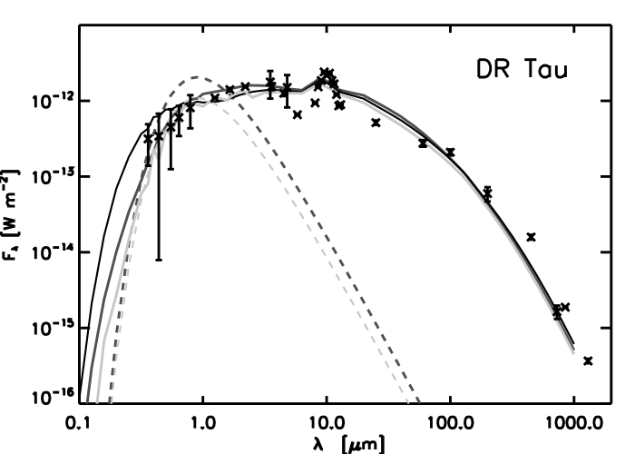
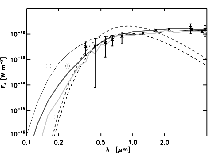
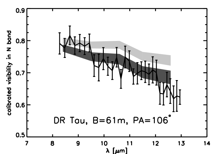
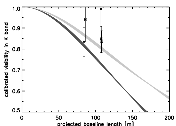
Figure 1: SED and MIR visibilities for a projected baseline of $B=60\,\mathrm{m}$ obtained from the measurements and our models (I), (II), and (III) of DR Tau. The model parameters are listed in Table 1 and Table 3. Upper row: SED and an enlargement showing photometric data from the visible up to the NIR wavelength range. The curves are ascribed to the specific models by numbers. Real photometric data are plotted with error bars. The dashed lines represent the intrinsic stellar flux of models (I), (II), and (III). Lower-left figure: The modeled visibilities were derived from the corresponding model images for the wavelengths of $8.5\,\mathrm{\mu m}$, $9.5\,\mathrm{\mu m}$, $10.6\,\mathrm{\mu m}$, $11.5\,\mathrm{\mu m}$, and $12.5\,\mathrm{\mu m}$. The colored bars represent intervals that limit the MIR visibilities $V(\lambda)$ for different position angles but the same inclination of the models (I: dark grey) and (III: light gray). For clarity, the visibilities obtained from model (II) are not shown but they are located between the results of model (I) and model (III). The measured data are included with error bars (black, solid line). Lower right figure: NIR visibilities as a function of the projected (effective) baseline length $B$ of an interferometer derived for a wavelength of $2.2\,\mathrm{\mu m}$ that result from model (III: light gray). Model (III) is the only model that fit all available data sets. The dark grey line represents the output of model (I) and (II), respectively. The measured NIR visibilities obtained with the PTI (Akeson et al. akeson (2005)) are included with error bars.

4.2 GW Ori

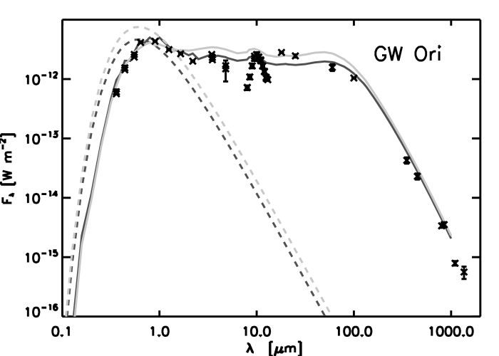
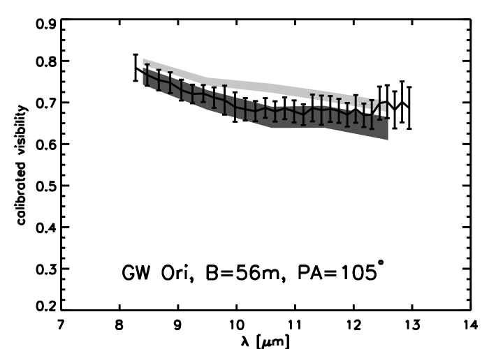
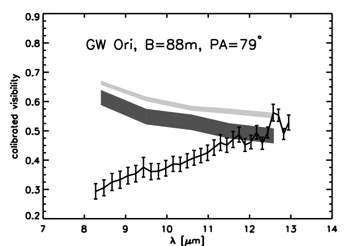
Figure 2: SED and MIR visibilities for the projected baselines of $B=56\,\mathrm{m}$ and $B=88\,\mathrm{m}$ obtained from the measurements and our model of GW Ori. The results of two different models are plotted that differ in the stellar luminosity (dark gray: $L_{\star}=40\,\mathrm{L_{\odot}}$, light gray: $L_{\star}=62\,\mathrm{L_{\odot}}$). The increasing visibility of the longest baseline $B=87\,\mathrm{m}$, which cannot be reproduced by our modeling approach, could point to a bright, truncated density structure in the inner disk region ($<5\,\mathrm{AU}$), although different scenarios are also possible.

As former millimeter measurements have shown (Mathieu et al. mathieuII (1995)) and can be confirmed by this study, the circumstellar disk around GW Ori is very massive, i.e., $M_{\mathrm{disk}}=1.0\,\mathrm{M_{\odot}}$. Furthermore, compared to other objects in this study, the disk of GW Ori has the largest outer radius $R_{\mathrm{out}}$. Besides the luminosity, all other stellar parameters and the accretion rate found in this study are consistent with the result of Calvet et al. (calvet (2004)), who analyzed the UV spectrum of this source. The accretion luminosity is $L_{\mathrm{acc}}=5\,\mathrm{L_{\mathrm{\odot}}}$ in our model. If an intrinsic stellar luminosity of $L_{\mathrm{\star}}=62\,\mathrm{L_{\mathrm{\odot}}}$ is used, as was determined by Calvet et al. (calvet (2004)), the resulting flux in K band would exceed the photometric measurement by $20\,\%$. In Fig. 2, the SED and MIR visibilities of a model with a stellar luminosity of $L_{\mathrm{\star}}=62\,\mathrm{L_{\mathrm{\odot}}}$ is also shown (model (II): gray curves/visibility bars). Although both the SED and the visibilities for $B=56\,\mathrm{m}$ can be reproduced, no model could be found that reproduces simultaneously the visibilities of a baseline of $B=88\,\mathrm{m}$. For spectroscopic measurements, Mathieu et al. (mathieu (1997)) found that GW Ori has a stellar companion at a projected separation $a_{\mathrm{sep}}$ between $a_{\mathrm{sep}}=1.08\,\mathrm{AU}$ and $a_{\mathrm{sep}}=1.18\,\mathrm{AU}$ and of stellar mass between $M_{\star}=0.5\,\mathrm{M_{\odot}}$ and $M_{\star}=1\,\mathrm{M_{\odot}}$. According to Mathieu et al. (mathieu (1997)), this companion creates a dust-free ring in the circumstellar disk between $r=0.17\,\mathrm{a_{\mathrm{sep}}}$ and $r=3.0\,\mathrm{a_{\mathrm{sep}}}$. By means of a theoretical investigation, Artymowicz & Lubow (artymowicz (1994)) determined an inner radius of $\sim$$2.3\,\mathrm{a_{\mathrm{sep}}}$ for the circumbinary disk of the system. They claimed that each component has its own circumstellar disk of outer radii of $0.46\,\mathrm{a_{\mathrm{sep}}}$ and $0.20\,\mathrm{a_{\mathrm{sep}}}$.

In our approach, the inner disk radius equals the sublimation radius ($R_{\mathrm{in}}=R_{\mathrm{sub}}$). We do not consider a dust-free inner gap as proposed by Mathieu et al. (mathieu (1997)) and Artymowicz & Lubow (artymowicz (1994)). However, in another model a dust-free, ring-shaped gap is cut in our disk model. We therefore assumed the same disk parameters $\beta$ and $h_{\mathrm{100}}$ for the circumbinary and circumstellar disk. The disk gap extends from the radius $0.5\,\mathrm{AU}$ to $3.0\,\mathrm{AU}$. In the latter model, we obtained the following results (not shown in the figure): the NIR flux obtained from this model decreases by $70\%$ and cannot fit the NIR range of the SED anymore. Although the modeled visibilities $V(\lambda)$ for the long baseline $B=87\,\mathrm{m}$ corresponds to a positive gradient, the visibilities for the short baseline $B=56\,\mathrm{m}$ decrease by $20\%$ across the complete N band. Any modifications of the radii that limit the disk gap could not even improve our model considering the measurements.

We assume that the disk gap is probably neither dust-free nor ring-shaped. In a theoretical study, it was shown that material streams between the circumbinary and the circumstellar disks guarantee the accretion onto each component (Günther & Kley guentherII (2002)). Even the stellar companion that is not implemented in our approach could affect the MIR visibilities and SED. A strong concentration of MIR intensity in the innermost disk regions that could not be spatially resolved with MIDI and an abrupt truncation of the MIR intensity distribution potentially caused by a disk gap result in the increase of the MIR visibility on long baselines.

To reveal the innermost disk region of GW Ori, more complicated modeling approaches as well as additional interferometric observations are essential. Measurements with the NIR interferometer AMBER at the VLTI, for instance, could provide information about the small-scale structures of the innermost regions that potentially deviate from axial symmetry.

4.3 HD 72106 B

HD 72106 B is the least well-studied object in our sample. In our modeling approach, we use a luminosity of $L_{\mathrm{\star}}=28\,\mathrm{L_{\odot}}$. This value results directly from a fit by a Planck function of temperature $T_{\mathrm{\star}}=9500\,\mathrm{K}$ (Schütz et al. schuetz (2005)) to the photometric measurements in U-, V- and R-band. Two properties make HD 72106 B a special object in our sample:

First, with an age of $10\,\mathrm{Myr}$, HD 72106 B is a relatively old T Tauri object with weak infrared excess. The equivalent width of the H$\alpha$ line that is smaller than $10\,$ Å (Vieira et al. vieira (2003)) is a sign of weak accretion. Our model of HD 72106 B consists of a passive disk without considering any accretion effects. For several T Tauri objects of similar age (e.g., TW Hya; s. Calvet et al. calvetII (2002)) an inner, dust-free gap in the range of $\lessapprox 1\,\mathrm{AU}$, i.e., larger than the sublimation radius could be detected. However, because the SED and MIR visibilities of HD 72106 B can be simulated by assuming that the inner edge of the (dust) disk equals the sublimation radius, a shift in the inner-disk edge to larger radii is not obvious.

Second, HD 72106 B is the infrared companion of HD 72106 A with a projected distance of $280\,\mathrm{AU}$. HD 72106 A has already developed into a main-sequence star (Wade et al. wade (2005)). The main component is probably responsible for the truncation of the outer disk around the B component considering an outer radius of $40\,\mathrm{AU}$. The small outer radius of the disk finally produces a strong decrease in the FIR flux (s. Fig 3).

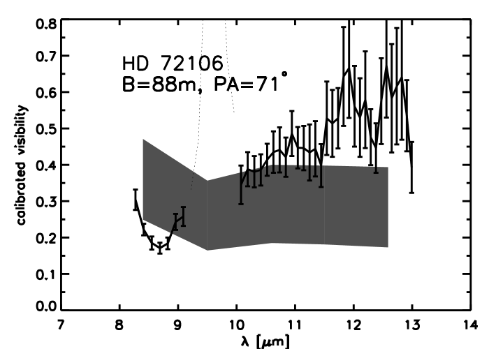
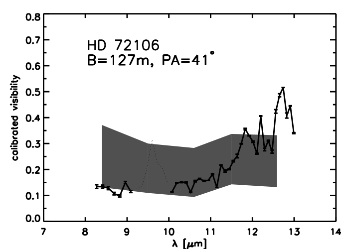
Figure 3: SED and MIR visibilities for the projected baselines of $B=88\,\mathrm{m}$ and $B=127\,\mathrm{m}$ that results from the measurements and our model of HD 72106 B. Dotted curves represent remnants of the telluric ozone band that could not be eliminated by the data reduction.

4.4 RU Lup

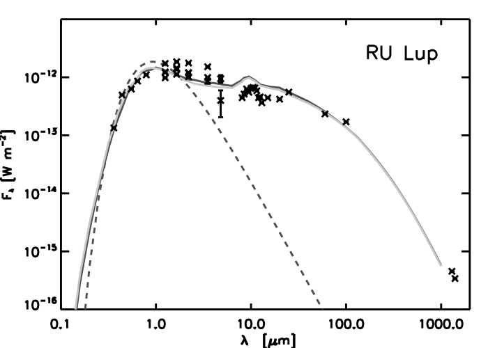
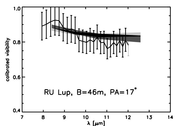
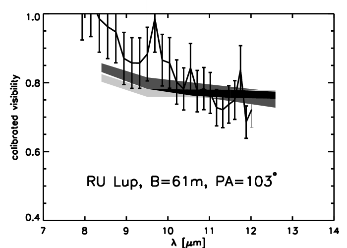
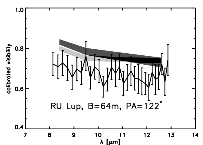
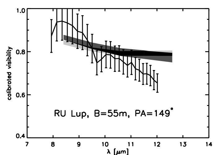
Figure 4: SED and MIR visibilities for the projected baselines of $B=46\,\mathrm{m}$, $B=55\,\mathrm{m}$, $B=61\,\mathrm{m}$, and $B=64\,\mathrm{m}$ obtained from the measurements and our model of RU Lup. For comparison, the light gray and dark gray colored curves/bars are results from two different models with and without disk gap, respectively. The black region of the visibility bars represents an intersection. The gap -if present- stretches from $2\,\mathrm{AU}$ to $4\,\mathrm{AU}$ according to Takami et al. (takamiII (2001)).

As Lamzin et al. (lamzin (1996)) has shown, RU Lup was at least temporarily a strongly accreting object. By analyzing its SED, they derived an accretion rate of $\dot{M}=3\times 10^{-7}\,\mathrm{M_{\odot}yr^{-1}}$. In this context, Reipurth et al. (reipurthII (1996)) found that the H$\alpha$ emission has broad wings of up to $900\,\mathrm{kms^{-1}}$ in width. Furthermore, the H$\alpha$ emission of RU Lup shows one of the broadest equivalent widths among T Tauri stars (Giovannelli et al. giovannelli (1995)). However, by considering SED and MIR visibilities, we can exclude such a high accretion rate $\dot{M}$. We determine a maximum value of $\dot{M}=1\times 10^{-8}\,\mathrm{M_{\odot}yr^{-1}}$ with an accretion luminosity of only $L_{\mathrm{acc}}=0.1\,\mathrm{L_{\odot}}$. Herczeg et al. (herczeg (2005)) found that $\dot{M}=(5\pm 2)\times 10^{-8}\,\mathrm{M_{\odot}yr^{-1}}$ which supports our result. A higher accretion rate produces a decrease in the MIR visibility because the irradiation of the disk increases. Simultaneously, the NIR and MIR flux would exceed the photometric measurements. Figure 4 represents our best-fit model with $\dot{M}=1\times 10^{-8}\,\mathrm{M_{\odot}yr^{-1}}$ (black curve/visibility bars). The stellar luminosity of $L_{\mathrm{\star}}=1.27\,\mathrm{L_{\odot}}$ corresponds to a value derived by Gras-Velázquez & Ray (gras-velazquez (2005)). It represents the average of previous measurements (Herczeg et al. herczeg (2005): $0.49\,\mathrm{L_{\odot}}$; Nürnberger et al. nuernberger (1997): $2.2\,\mathrm{L_{\odot}}$). A model that simulates the flux in the N band, i.e., the silicate feature, could not be found. The relative deviation in the MIR range is $37\%$. The visibilities obtained on the baselines $B=61\,\mathrm{m}$ and $B=65\,\mathrm{m}$ and for similar position angles significantly differ, which could be due to a measurement error.

Based on spectro-astrometric observations, Takami et al. (takamiII (2001)) suggested that an inner gap in the circumstellar disk of RU Lup exists between $\sim$$2\,\mathrm{AU}$ and $\sim$$4\,\mathrm{AU}$ ($20$-$30\,\mathrm{mas}$) as justified by the following arguments. Because of the positional displacement of the extended wings, the emission of forbidden lines such as [OI] and [SII] in the spectra of RU Lup is assumed to arise in a collimated large-scale outflow. The apparent lack of redshifted line components results from an obscuration of the dorsal outflow by the circumstellar disk (Eislöffel et al. eisloeffel (2000)). Takami et al. (takamiII (2001)) found that the H$\alpha$ line in the spectrum of RU Lup, which is evident predominatly in the innermost regions, shows both blueshifted and redshifted wings. This finding is explained by an inner disk gap that allows regions behind the disk to be observed. The gap could be evoked by an unseen (planetary) companion. Since the wings of the H$\alpha$ line shows the same positional displacement as the forbidden lines, Takami et al. (takamiII (2001)) suggested that the H$\alpha$ line originates predominantly in the outflow.

Similar to our modeling approach of GW Ori, we defined a dust-free gap in the disk model that is presented in Fig. 4 (Tables 1,3). The gap size was varied using values of $R_{\mathrm{in}}$ of up to $3\,\mathrm{AU}$ for the inner gap radius, and $3\,\mathrm{AU}$ and $5\,\mathrm{AU}$ for the outer gap radius. An outflow was not considered in our model. The resulting changes can be summarized as follows: as shown in Fig. 4, a gap lowers the NIR flux by $\sim$$7$%. We note that the NIR flux is highly variable during a year (Giovannelli et al. giovannelli (1995)). Previous photometric measurements (Giovannelli et al. giovannelli (1995)) would be consistent with lower NIR fluxes. A disk gap as used here would even lower the MIR flux and slightly improve our fit to the N band. The MIR visibility simultaneously decreases at wavelengths $<10.5\,\mathrm{\mu m}$ as the relative MIR flux contribution of outer disk regions in relation increases. For longer wavelengths $>10.5\,\mathrm{\mu m}$, the disk becomes more compact as the visibilities slightly increase. Our visibility measurements are inconsistent with a disk gap and an inner radius of $r=R_{\mathrm{in}}$, only, but a gap of between $2\,\mathrm{AU}$ and $4\,\mathrm{AU}$ fits the visibility data as well as the model without gap.

Although there are observational hints for a disk gap, we are unable to conclude whether the model with a disk gap of inner radius $\gtrapprox 2\,\mathrm{AU}$ or a model disk without gap provide a closer fit to the data. Further interferometric observations and simultaneous photometric measurements in the NIR wavelength range would allow a final confirmation or rejection of the presence of a gap in the disk of RU Lup.

4.5 HBC 639

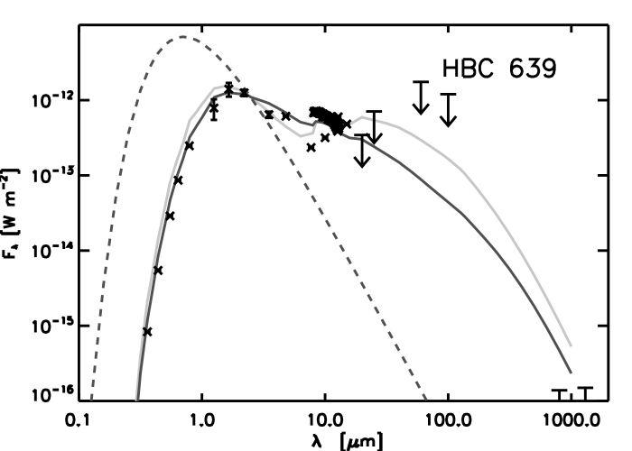
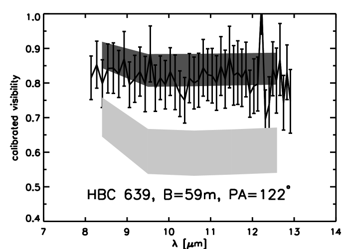
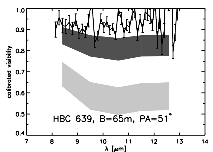
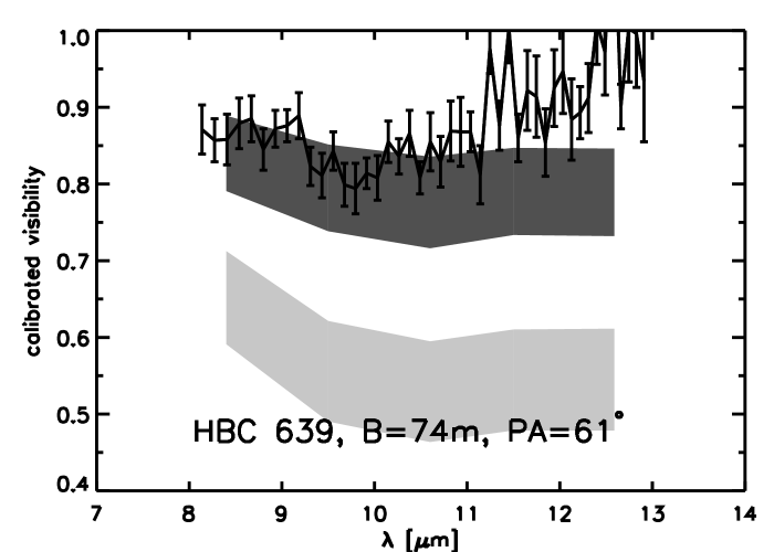
Figure 5: SED and MIR visibility for the projected baselines of $B=59\,\mathrm{m}$, $B=65\,\mathrm{m}$, and $B=74\,\mathrm{m}$ obtained from the observations and the model of HBC 639. We assume that the photometric measurements in the FIR range are ascribed to the infrared companion. The light gray curves/bars represent a model with a disk parameter $\beta=1.1$ instead of using $\beta=1.0$ (grey colored curves/bars).

Apart from HD 72106 B, the source HBC 639 is the only object where accretion has not been considered. Although HBC 639 has an age of between $1$ and $3\,$million years (Gras-Velázquez & Ray gras-velazquez (2005)), we can neglect the derived accretion rate (Prato et al. prato (2003)), for which we estimate an upper limit of $\dot{M}<1\times 10^{-8}\,\mathrm{M_{\odot}yr^{-1}}$. Since the equivalence width of the H$\alpha$ line is smaller than $10\,$Å, HBC 639 is not a classical T Tauri star but belongs to the class of weak-line T Tauri stars.

The parameter combination listed in Table 3 could reproduce the MIR visibilities. However, this model produces a strong decline in the FIR flux and is therefore unable to reproduce the photometric upper limits in the FIR range. HBC 639 has an infrared companion at a projected distance of $320\,\mathrm{AU}$ (s. Appendix A). The strong decline in the FIR flux could be explained by the presence of an infrared companion that truncates the outer-disk region of the main component. In the latter case, the measured flux in the FIR (s. Fig. 5) can mainly be ascribed to this infrared companion. The companion is again a binary, as well, and deeply embedded in a circumbinary envelope.

A larger value for the disk parameter $\beta$ results in a more flared disk. Outer disk regions can be more effectively heated and the intensity distribution in the MIR range therefore decreases less strongly. A consequence is a decrease in the MIR visibilities. Fig. 5 also shows the results of a model with $\beta=1.1$ for which none of the other parameters were modified. We note that the visibilities decrease by at least $10\%$ for all baselines and the FIR flux increases by almost a factor of $2$.

4.6 S CrA N

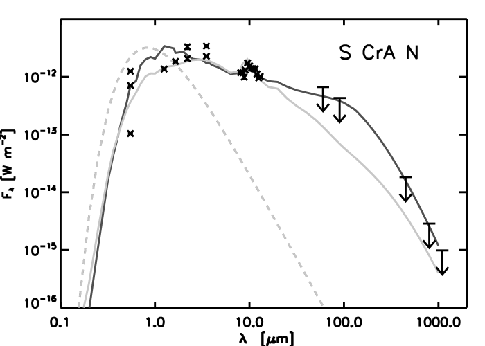
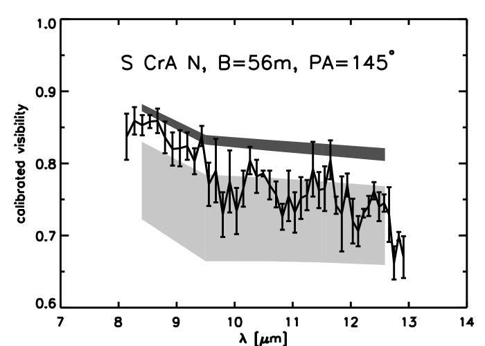
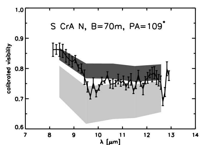
Figure 6: SED and MIR visibilities for the projected baselines of $B=56\,\mathrm{m}$, and $B=70\,\mathrm{m}$ obtained from the observations and the model of S CrA N (dark grey line/colored bars). A second model with $\beta=0.90$, and $h_{\mathrm{100}}=12\,\mathrm{AU}$ (light gray lines/colored bars) can even improve the reproduction of the NIR fluxes.

Only the photometric measurements in the NIR and MIR range can exclusively be ascribed to the Northern component of this binary. All other photometric measurements could not spatially resolve the individual components of the binary system. The visual extinction $A_{\mathrm{V}}$ and the effective stellar temperature $T_{\mathrm{\star}}$ used in the model are within the $1\,\sigma$-deviations ($1.0\,\mathrm{mag}$ and $400\,\mathrm{K}$) of the previously derived results of Prato et al. (prato (2003)). The NIR flux that results from our model deviates by $60\%$ from the measurements (s. Fig. 6). The accretion luminosity is equal to $L_{\mathrm{acc}}=0.7\,\mathrm{L_{\mathrm{\odot}}}$.

A second model for S CrA N (grey curve/bars in Fig. 6) with $\beta=0.90$ and $h_{\mathrm{100}}=12\,\mathrm{AU}$ does not reproduce the visibility measurements as well as the first model (deviations from the measurements are $6\%$) but the SED for $\lambda<14\,\mathrm{\mu m}$ can be simulated more accurately. In contrast to HBC 639, the FIR flux must then originate in the Southern component. Furthermore, to reproduce the visual wavelength range, the second model still allows an inclination angle of up to $\vartheta\lessapprox 45\degr$, while only lower inclinations angles of $\vartheta<10\degr$ can be used in the first model.

4.7 S CrA S

The Southern component of S CrA is the fainter component in the NIR and MIR wavelength range. An investigation of the Br$\gamma$ line showed that this component is as active as the Northern component (Prato & Simon pratoII (1997)). A value for the accretion rate had not yet been derived. The accretion luminosity in our model is $L_{\mathrm{acc}}=0.2\,\mathrm{L_{\mathrm{\odot}}}$. The corresponding accretion rate of $\dot{M}=4\times 10^{-8}\,\mathrm{M_{\odot}yr^{-1}}$ is already an upper limit because higher values would produce an increase in the disk irradiation and a decrease in the visibilities. If accretion is not considered in our model, the MIR visibilities increase by only $2\%$. Figure 7 represents our best-fit model.

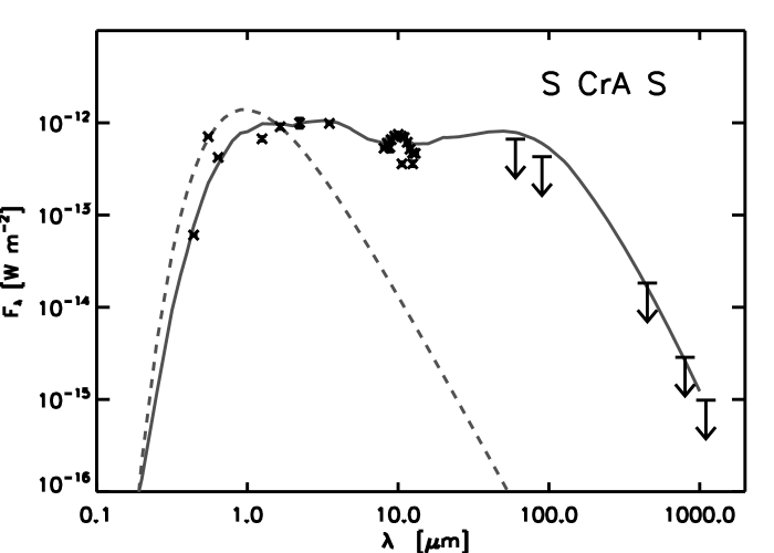
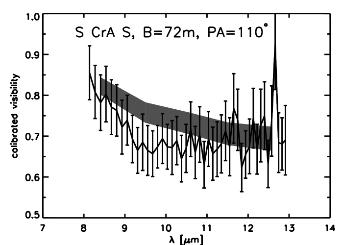
Figure 7: SED and MIR visibilities for a projected baseline of $B=72\,\mathrm{m}$ obtained from the measurements and our best model for S CrA S.

5 Radial gradient of the dust composition in circumstellar disks around T Tauri stars

For each single interferometric observation with MIDI and for each single telescope, one uncorrelated N band spectrum can be obtained. For each interferometric observation, we also obtained a correlated spectrum reflecting the flux emitted by regions that are not spatially resolved by the interferometer. An increasing effective baseline length $B$ of the interferometer results in a higher resolution. The uncorrelated, i.e., single-dish spectra as well as the correlated spectra contain spectral contributions of the N band from the entire disk, while the contributions from the hotter and brighter, i.e., inner regions increase with increasing effective baseline length $B$ assuming a homogeneous, axial-symmetric disk. It was shown by Schegerer et al. (schegerer (2008)) that the local silicate dust composition in the circumstellar disk around RY Tau depends on the radial distance from the star, i.e., the relative contribution of crystalline and large dust grains increases towards the star. Small and large dust grains are assumed to have a radius of $0.1\,\mathrm{\mu m}$ and $1.5\,\mathrm{\mu m}$, respectively. In the following, we investige whether a corresponding correlation between radial location and dust composition can also be found in the T Tauri stars of our sample.

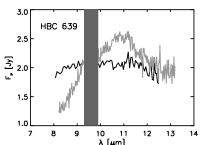
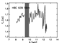
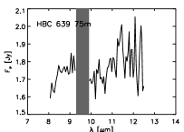
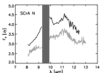
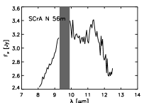
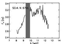
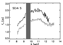
Figure 9: Continuation of Fig. 8.

The (averaged) uncorrelated spectra and the correlated spectra are shown in Fig. 8. All uncorrelated and correlated spectra exhibit the silicate emission feature apart from the correlated spectra of HD 72106 and HBC 639 that were obtained with the longest interferometric baseline. The uncorrelated spectra obtained during different nights differ in absolute flux scale by $4$% for S CrA N and up to $35$% for GW Ori, while the shape of the spectra does not change. We assume that the variation in the absolute flux scale of a spectrum is caused by an erroneous photometric calibration during data reduction. Przygodda (przygoddaII (2004)) indeed confirmed that the scale factor of the photometric calibration can vary by more than $15$% during a single night. If available, spectra acquired by the Thermal Infrared Multi Mode Instrument 2 (TIMMI 2) at ESO’s observatory La Silla (Przygodda et al. przygodda (2003); Schegerer et al. schegererI (2006)) are also plotted in Figs. 8 and 9. The spectra obtained with TIMMI 2 can be used in the following comparison. With respect to the TIMMI 2 data, the shapes of the uncorrelated MIDI spectra are largely preserved for GW Ori (deviation: $6$%), RU Lup ($9$%), S CrA N ($18$%), and S CrA S ($25$%) and differ only in absolute scale. However, the shapes of the spectra of DR Tau, and of HBC 639 in particular, differ significantly in a way that could be due to an intrinsically temporal variation. We note that the TIMMI 2 spectra were obtained $\sim$$3\,$years before our MIDI observations. However, the difference could also be caused by a doubling of the spatial resolution power using a $8.2\,\mathrm{m}$-single-dish of MIDI in contrast to the $3.6\,\mathrm{m}$-telescope of TIMMI 2. Therefore, observations with a single-dish of the VLTI allows us to observe exclusively more central regions of the source, where more evolved grains are assumed to exist. We should mention that a spatial resolution of $\sim$$43\,\mathrm{AU}$ at a distance of $\sim$$140\,\mathrm{pc}$ can theoretically be achieved with a single-dish observation with the VLT. With respect to the TIMMI 2 spectrum, the flattening of the MIDI spectrum of HBC 639 could originate from an increase in the mass contribution of large silicate grains in the more central regions considering their specific absorption efficiency $\kappa$ (Dorschner et al. dorschner (1995)). Our latter assumption is also confirmed by the correlated spectra of the objects HD 72106 B and HBC 639 obtained with the longest interferometric baseline. These spectra are flat and do not show any silicate emission band. We refer to a study of Min et al. (min (2006)), where it was found that the silicate band disappears if the averaged dust grain size exceeds $\sim$$4\,\mathrm{\mu m}$.

The origin of the evolved dust contributing to the TIMMI 2 spectra can be derived by considering the following comparison with the MIDI spectra. A black body $B(\nu,T)$ that represents the putative underlying continuum (Schegerer et al. schegererI (2006)) and is fitted to the extended wings of the emission features $F(\nu)$ of TIMMI 2 as well as correlated and uncorrelated MIDI spectra, is subtracted from N band. We derive normalized features using:

$$\hfill{}F_{\mathrm{norm}}(\nu)=1+\frac{(F(\nu)-B(\nu,T))}{B(\nu,T)}.\hfill{}$$ (4)

This normalization procedure preserves the shape of the emission feature (Przygodda et al. przygodda (2003)). According to Schegerer et al. (schegererI (2006)), the contributions of amorphous and crystalline dust to the TIMMI 2 spectra are determined using a $\chi^{2}$ fitting routine, where the absorption efficiencies $\kappa$ of dust are linearly combined. In the context of the latter findings, we additionally subtract the contribution of small amorphous dust from the normalized TIMMI 2 spectra and compare the resulting spectra with the normalized uncorrelated and correlated MIDI spectra. In Figs. 10 and 11, we only compare the normalized TIMMI 2 spectra with both the normalized uncorrelated and normalized correlated MIDI spectra obtained with the longest effective baseline length. With respect to our results, all sources can be divided into three classes:

1. The normalized TIMMI 2 spectra reproduce well the normalized uncorrelated and normalized correlated MIDI spectra. The evolved grains that contribute to the TIMMI 2 spectra originate therefore in more central regions. Since the normalized TIMMI 2 spectra similarly correspond to the normalized uncorrelated and normalized correlated MIDI spectra, a further evolution of dust in regions that MIDI is able to study, cannot be determined. DR Tau and S CrA N belong to this class.

2. The normalized TIMMI 2 and MIDI spectra of HBC 639 differ at $\sim$$10.8\,\mathrm{\mu m}$, where the crystalline compound enstatite generally shows a specific emission feature. If the remaining feature at $\sim$$10.8\,\mathrm{\mu m}$ in the normalized TIMMI 2 spectrum can be ascribed to enstatite, our comparison suggests that enstatite has its origin in more outer disk regions. These outer regions can already be resolved with a single-dish of MIDI and do not appear in the MIDI spectra. S CrA S could also be ascribed to this class by considering its correlated, normalized spectra. This result is based on the assumption that the spectral resolution power of MIDI is high enough to resolve the $\sim$$10.8\,\mathrm{\mu m}$ feature of enstatite only in the inner regions.

3. An increasing flattening of the emission feature and an increasing amplitude of the forsterite feature at $11.3\,\mathrm{\mu m}$ with increasing baseline length $B$ suggest grain evolution towards more central regions (e.g., GW Ori). The comparison with the corresponding normalized TIMMI 2 spectra shows, however, that the contribution of small amorphous dust grains, emitting a triangular emission feature with the maximum at $9.8\,\mathrm{\mu m}$, is still large even in the correlated spectrum that were obtained with the longest baselines. GW Ori, RU Lup, and S Cr A S belong to this class.

We note that all of these findings are based on the assumption that the underlying continuum of the emission feature can be represented by a single black body. This procedure is circumstantially discussed in Schegerer et al. (schegererI (2006)).

Considering a measurement error in the visibility of $\sigma\approx 0.1$ as well as the low signal-to-noise ratio of $\sim$$4$ and the low spectral resolution reached, we avoid fitting the uncorrelated and correlated MIDI spectra using a linear combination of different-sized, amorphous and crystalline silicate grains. The latter procedure was presented by Schegerer et al. (schegererI (2006)) and Schegerer et al. (schegerer (2008)). However, we conclude that the local silicate dust composition in the circumstellar disks around the T Tauri objects of our sample depends on the radial disk location. Features of crystalline and large silicate grains indeed originate predominantly in more central disk regions of several AUs in size. However, the features of enstatite could originate in more outer regions, and the spectral contribution of small, non-evolved dust grains from the inner disk region could remain high.

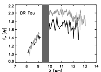
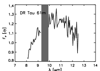
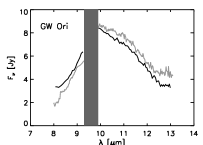
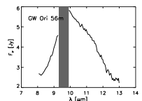
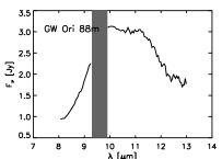
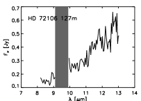
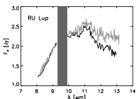
Figure 8: Uncorrelated and correlated N band spectra obtained from the objects that were observed with MIDI for this study (black lines). Correlated spectra are designated by the additional information about the baseline length $B$ (Table 2). Because of the remaining ozone band in several spectra the wavelength interval from $\sim$$9.3\,\mathrm{\mu m}$ up to $\sim$$9.9\,\mathrm{\mu m}$ is cut and underlaid with gray color. The gray lines represent data formerly obtained with TIMMI 2 (Przygodda et al. przygodda (2003); Schegerer et al. schegererI (2006)).

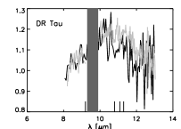
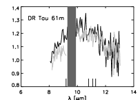
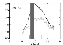
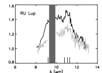
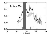
Figure 10: Uncorrelated and correlated MIDI spectra after subtraction of a black body that represents the underlying continuum and is fitted to the extended wings of the emission features (black lines). The gray curves represent TIMMI 2 data (Przygodda et al. przygodda (2003)) after subtraction of a black body and the spectral contribution of small amorphous dust grains found in the preceeding study of Schegerer et al. (schegererI (2006)). For clarity, we only show the results obtained for the single-dish spectra and the correlated spectra that were obtained for the longest effective baseline length. The vertical lines designate features of enstatite (at $9.2\,\mathrm{\mu m}$, $10.8\,\mathrm{\mu m}$, and $11.1\,\mathrm{\mu m}$) and forsterite (at $11.3\,\mathrm{\mu m}$).

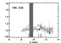
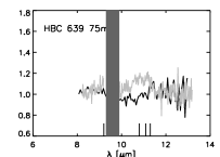
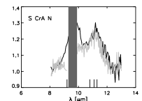
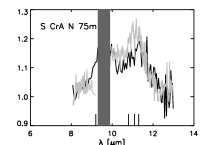
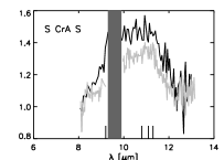
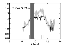
Figure 11: Continuation of Fig. 10.

6 Summary

We have presented MIR visibilities of seven pre-main-sequence stars observed with MIDI at the VLTI. We modeled the SEDs and the spectrally resolved MIR visibilities of these YSOs, and in particular T Tauri objects. The density distributions of the circumstellar disks were derived using the parametrized approach of Shakura & Sunyaev (shakura (1973), Eq. 1). The results of this study are:

1. All objects could be spatially resolved with MIDI.

2. We showed that the results of highly spatially resolved observations in the MIR range probing small-scale structures in the range of several AUs, and the SED from the visual to the millimeter wavelength range can simultaneously be reproduced by a single model except for one source (see vi.). We note that the SED does not generally provide any spatial information. The number of models that simulate the SED, solely, can be strongly reduced by the measurements with MIDI. Furthermore, the results of previous investigations based on large-scale observations in the range of several $10\,\mathrm{AUs}$, were confirmed by our modeling results in most cases. Any differences between the results of previous measurements and our modeling approach (e.g., the accretion rate of RU Lup) could be caused by a time-dependent variability.

3. For five of seven objects, the modeling approach of a purely passive disk is insufficient to reproduce the SED and the MIR visibilities of the sources. The implementation of accretion effects also significantly improves the simulation of the measurements.

4. For two objects in this study, i.e., HD 72106 B and HBC 639, the approach of a passive disk without accretion is sufficient. HD 72106 B is $10\,$million years old and its low accretion rate and high mass contributions from crystalline and large dust grains, have already been mentioned in previous investigations (Vieira et al. vieira (2003); Schütz et al. schuetz (2005)). In contrast, HBC 639 is still a relatively young object (Gras-Velázquez & Ray al. gras-velazquez (2005)) but belongs to the class of weak-line T Tauri stars.

5. For some targets (e.g., DR Tau, and S CrA N), the MIR data do not constrain all model parameters. However, further modeling constraints can be obtained from additional measurements, e.g., NIR visibilities as shown for our modeling approach for DR Tau, where PTI data were additionally taken into account.

6. The modeling result for the source GW Ori illustrates the need for an individual extension to our approach. According to Mathieu et al. (mathieu (1997)), GW Ori has a stellar companion at a (projected) distance of $\sim$$1\,\mathrm{AU}$. Therefore, in a second model we considered a combination of a circumstellar and circumbinary disk. The circumstellar and circumbinary disk are determined by the same disk parameters $\beta$ and $h_{\mathrm{100}}$ and are seperated by a dust-free gap. However, a model that reproduces all the measurements could not be found. We recommend acquiring additional high spatial resolution observations including phase measurements to clarify the complex inner-disk structure of this object.

7. Our measurements of RU Lup can be simulated equally with an active disk model with or without a dust-free gap. A disk model with a gap was formerly proposed by Takami et al. (takamiII (2001)) based on spectro-astrometric observations.

8. Each single component of the binary system S CrA could be seperately observed with MIDI. Considering inner disk regions on small scales that could be resolved with MIDI, basic differences between this binary system and other objects in our sample without a companion could not be found. Only the SEDs of the sources HD 72106 B, HBC 639, and S CrA N that decline strongly at $\lambda>10\,\mathrm{\mu m}$ support the idea that a stellar companion truncates the outer disk regions of this sources.

9. The relative mass contribution of evolved dust in the systems of fainter T Tauri objects is higher in the inner disk regions close to the central star than in the outer regions. However, enstatite could already be enriched and stimulated in outer disk regions and the spectral contribution from non-evolved dust grains could still be high in the inner regions.

Appendix A Previous measurements:

DR Tau: The $2.5\,$million-year-old object DR Tau belongs to the Taurus-Auriga star-forming region at a distance of $\sim$$140\,\mathrm{pc}$ (Siess et al. siess (1999)). Numerous publications illustrate that DR Tau is one of the most well-studied T Tauri objects. Strong veiling has been found in the visual and NIR wavelength range: the flux in V band, for instance, exceeds the intrinsic stellar flux by a factor of five (Edwards et al. edwards (1993)). Apart from the excessive flux in the visual, the profiles of several emission lines, such as the Pf$\gamma$-line, points to material accreting onto the central star while the profiles of further emission lines such as the He I line (Kwan et al. kwan (2007)) and the H$\alpha$ lines (Vink et al. vink (2005)) are evidence of outflowing stellar/disk winds. Based on a modeling study, Edwards et al. (edwards (1993)) determined an accretion rate of $\dot{M}=7.9\times 10^{-6}\,\mathrm{M_{\odot}yr^{-1}}$, while a mass of $\dot{M}_{\mathrm{wind}}=2.5\times 10^{-9}\,\mathrm{M_{\odot}yr^{-1}}$ is lost by stellar/disk winds. A strongly collimated outflow was also found by Kwan & Tademaru (kwanII (1988)). DR Tau is photometrically and spectrally variable on short terms, i.e., in the range of weeks ($\Delta V=1.3\,\mathrm{mag}$; Grankin et al. grankin (2007); Eiroa et al. eiroa (2002); Smith et al. smithIII (1999)). This variability is also ascribed to the formation and movement of stellar spots on this star (Ultchin et al. ultchin (1997)).
GW Ori: GW Ori, also known as HD 244138, belongs to the star-forming region B $30$ in a ring-shaped molecular cloud close to $\lambda$ Ori. According to Dolan & Mathieu (dolan (2001)), the ring shape has its origin in a central supernova explosion $1\,$million years, ago. As GW Ori is $\sim$$1\,$million years old (Mathieu et al. mathieuIII (1991)), the supernova explosion could cause the formation of this object. Considering a stellar luminosity of several tens of solar luminosities (Mathieu et al. mathieu (1997); Calvet et al. calvet (2004)), GW Ori is one of the most luminous YSOs with a spectral type of G$0$. Using theoretical evolutionary tracks, a stellar mass of $2.5\,\mathrm{M_{\mathrm{\odot}}}$ (Mathieu et al. mathieuIII (1991)) and $3.7\,\mathrm{M_{\mathrm{\odot}}}$ (Calvet et al. calvet (2004)) could be derived. GW Ori is a spectroscopic binary (Mathieu et al. mathieuIII (1991)). The companion with a mass of $0.5\,\mathrm{M_{\odot}}$ up to $1\,\mathrm{M_{\odot}}$ orbits the primary at a projected distance of $\sim$$1\,\mathrm{AU}$ in $242\,$days. Mathieu et al. (mathieu (1997)) used two different modeling approaches to reproduce the SED of this system. In their first approach, the secondary creates a (gas and dust free) gap between $0.17\,\mathrm{AU}$ and $3.3\,\mathrm{AU}$. Their second modeling approach, where the circumbinary disk was replaced by a spherical envelope, disagreed with subsequent millimeter measurements at the James Clerk Maxwell Telescope (Mathieu et al. mathieuII (1995)). A disk mass of $0.3\,\mathrm{M_{\odot}}$ could be derived using the latter set of millimeter measurements, where the object could be spatially resolved. An outer radius of $500\,\mathrm{AU}$ and an inclination angle of $\vartheta\approx 27\degr$ were determined. Artymowicz & Lubow (artymowicz (1994)) showed that the disk gap of GW Ori proposed by Mathieu et al. (mathieuIII (1991)) cannot be explained by a theoretical modeling study of tidal forces. Calvet et al. (calvet (2004)) measured an accretion rate of $\dot{M}>2.5\times 10^{-7}\,\mathrm{M_{\odot}a^{-1}}$, but the source does not reveal any veiling in the visual. To stabilize a high accretion rate for several $100,000\,$years, Gullbring et al. (gullbring (2000)) proposed the existence of an additional massive envelope where an inner cavity enables the observation of the inner disk edge. GW Ori is only weakly variable ($\Delta V=0.2\,\mathrm{mag}$; Grankin et al. grankin (2007)). Mathieu et al. (mathieuIII (1991)) pointed to a second companion with a period of $1,000\,$days that was found by the movement of the center of gravity in the system.
HD 72106 B: The object HD 72106 is a visual binary (angular distance $0.78\arcsec$, $PA=199.8\degr$) in the Gum nebula at a distance of $288^{+490}_{-204}\,\mathrm{pc}$ (Torres et al. torres (1995); Hartkopf et al. hartkopf (1996); Fabricius & Makarov fabricius (2000)). The H$\alpha$-emission as well as the infrared excess are ascribed to the visually fainter B-component ($\Delta V=0.8\,\mathrm{mag}$), while the A component already belongs to the main sequence (Vieira et al. vieira (2003); Wade et al. wade (2005)) and shows a strong magnetic field that was found with spectropolarimetry (Wade et al. wade (2005); Wade et al. wadeII (2007)). The faint H$\alpha$ emission line as well as the broad $10\,\mathrm{\mu m}$ silicate emission band that can be compared with the silicate band of the comets Hale-Bopp and Halley point to the advanced evolutionary status of the B component as a YSO (Vieira et al. vieira (2003); Schütz et al. schuetz (2005)). In particular, Schütz et al. (schuetz (2005)) found larger amounts of enstatite ($\sim$$50\%$) that effectively contributes to the silicate band. This large spectral contribution of enstatite has only been found for the evolved Herbig Ae/Be objects, HD 100546 and HD 179218, so far. Folsom (folsom (2007)) intensively studied this binary system.
RU Lup: RU Lup is a classical T Tauri star in the star-forming region Lupus. Visual and millimeter measurements showed that the object does not have a (remaining) circumstellar envelope (Giovannelli et al. giovannelli (1995); Lommen et al. lommen (2007)). A secondary could not be found with speckle interferometry down to a minimal distance of $0.1\arcsec$ in the NIR range (Ghez et al. ghez (1997)) and with the Hubble Space Telescope (Bernacca et al. bernacca (1998)). Broad visual emission lines as well as flux variations in the U and V band are evidence of accreting material. Lamzin et al. (lamzin (1996)) determined a mass accretion rate of $\dot{M}=3\times 10^{-7}\,\mathrm{M_{\mathrm{\odot}}yr^{-1}}$. The stellar magnetic field of the object has a strength of $3\,\mathrm{kG}$ (Stempels et al. stempels (2007)). Absorption lines shifted to longer wavelengths results from an outflowing stellar wind (Herczeg et al. herczeg (2005)).
HBC 639: HBC 639, also known as DoAr 24 E, belongs to the star-forming region $\rho$ Ophiuchi. It is a class II object (McCabe et al. cabe (2006)) with an age of between $1$ and $3$ million years (Gras-Velázquez & Ray gras-velazquez (2005)). Because the H$\alpha$ line reveals an equivalent width of $\sim$$5\,$Å, HBC 639 is a weak-line T Tauri object, where the circumstellar material has evolved more rapidly than in classical T Tauri stars of similar age. However, the infrared excess points to a remaining circumstellar disk in the system. The accretion rate inferred from the width of the Pa$\beta$ and Br$\gamma$ lines is low: $\dot{M}=6\times 10^{-9}\,\mathrm{M_{\mathrm{\odot}}yr^{-1}}$ (Natta et al. natta (2006)). HBC 639 has an infrared companion at an angular distance of $2\arcsec$ ($320\,\mathrm{AU}$ for $160\,\mathrm{pc}$) and a position angle of $PA=150\degr$ measured from North to East (Reipurth & Zinnecker reipurth (1993)). The brightness of the secondary increases in the infrared and exceeds the brightness of the primary already in L band (Prato et al. prato (2003)). Chelli et al. (chelli (1988)) assumed that the primary effectively contributes only to the NIR and MIR flux of the system. Polarimetric measurements in the K band showed that both components have a circumstellar disk with almost identical position angles ($PA\approx 12,5\degr$; Jensen et al. jensen (2004)). The companion is a class I object and active (Prato et al. prato (2003)). Using the speckle-interferometric technique in K band, Koresko (koresko (2002)) found a second companion close to the secondary. Both latter companions have a similar brightness in K band.
S CrA: The source S CrA belongs to the Southern Region of the Corona Australis Complex (e.g., Chini et al. chini (2003)). The source was already defined as a T Tauri object by Joy et al. (joy (1945)) who pointed to an infrared companion at a projected distance of $169\,\mathrm{AU}$ and at a position angle of $PA=149\degr$ (Joy & Biesbrock joyII (1944); Reipurth & Zinnecker reipurth (1993)). Highly spatially resolved observations in the NIR wavelength range showed that both objects have an active circumstellar disk (Prato et al. prato (2003)). The spectral lines of both objects indicate that they have similar shapes and depths. Both components are probably coeval (Takami et al. takami (2003)). S CrA is a YY Ori object, i.e., the emission lines are asymmetric and shifted to longer wavelengths. These lines arise from material that accretes onto the central star. The measured spectral variability is another hint of non-continuous accretion process. Prato & Simon (pratoII (1997)) showed that only an infalling circumbinary envelope provides enough material for accretion in the long-term.

Table 4: Photometric flux measurements of DR Tau.

wavelength [$\mathrm{\mu m}$]	flux [Jy]	Ref.
$0.36$	$0.038\pm 0.021$	1
$0.44$	$0.050\pm 0.049$	1
$0.55$	$0.083\pm 0.060$	1
$0.64$	$0.13\pm 0.06$	1
$0.79$	$0.21\pm 0.01$	1
$1.25$	$0.45\pm 0.01$	2
$1.65$	$0.77\pm 0.04$	2
$2.20$	$1.13\pm 0.02$	2
$3.50$	$2.07\pm 0.82$	1
$3.60$	$1.86\pm 0.20$	7
$4.50$	$1.89\pm 0.15$	7
$4.80$	$2.41\pm 1.10$	1
$5.80$	$1.27\pm 0.01$	3
$8.00$	$1.77\pm 0.20$	7
$12.0$	$3.16\pm 0.25$	4
$25$	$4.30\pm 0.29$	4
$60$	$5.51\pm 0.54$	4
$100$	$6.98\pm 0.63$	4
$200$	$3.98\pm 0.84$	5
$450$	$2.38\pm 0.17$	6
$729$	$0.40\pm 0.08$	8
$850$	$0.53\pm 0.01$	6
$1300$	$0.16\pm 0.01$	6

References – 1: Kenyon & Hartmann (kenyon (1995)); 2: 2 MASS catalogue (Cutri et al. cutri (2003)); 3: Hartmann et al. (hartmannIV (2005)); 4: Gezari catalogue (gezari (1999)); 5: ISO data archive; 6: Andrews & Williams (andrewsII (2005)); 7: Robitaille et al. (robitaille (2007)); 8: Beckwith et al. (beckwith (1990))

Table 5: Photometric flux measurements of GW Ori. The value that is marked with the symbol “$\downarrow$” is an upper flux limit.

wavelength [$\mathrm{\mu m}$]	flux [Jy]	Ref.
$0.36$	$0.068\pm 0.014$	1
$0.44$	$0.21\pm 0.02$	1
$0.55$	$0.43\pm 0.02$	1
$0.70$	$0.61\pm 0.03$	1
$0.90$	$0.82\pm 0.05$	1
$1.25$	$1.31\pm 0.04$	2
$1.65$	$1.47\pm 0.04$	2
$2.20$	$1.47\pm 0.04$	2
$3.50$	$2.45\pm 0.09$	3
$4.80$	$2.7\pm 1.2$	4
$18$	$17\pm 3$	5
$25$	$20.5\pm 1.2$	6
$60$	$31.5\pm 4.1$	6
$100$	$35^{\downarrow}$	6
$350$	$5.0\pm 0.6$	7
$450$	$3.5\pm 0.4$	7
$800$	$0.9\pm 0.1$	7
$850$	$1.0\pm 0.1$	7
$1100$	$0.29\pm 0.03$	7
$1360$	$0.26\pm 0.06$	7

References – 1: Calvet et al. (calvetII (2002)); 2: 2 MASS catalogue (Cutri et al. cutri (2003)); 3: Rydgren & Vrba (rydgrenII (1983)); 4: Cohen & Schwartz (cohen (1975)); 5: Cohen (cohenIV (1973)); 6: IRAS catalogue (iras (1985)); 7: Mathieu et al. (mathieuII (1995))

Table 6: Photometric flux measurements of HD 72106 B. The value that is marked with the symbol “$\downarrow$” is an upper limit.

wavelength [$\mathrm{\mu m}$]	flux [Jy]	Ref.
$0.36$	$0.80$	1
$0.44$	$1.67$	1
$0.55$	$1.45$	1
$0.79$	$1.32$	1
$0.90$	$0.89$	1
$1.23$	$0.61$	3
$1.25$	$0.67\pm 0.01$	2
$1.63$	$0.45$	3
$1.65$	$0.50\pm 0.02$	2
$2.19$	$0.41$	3
$2.20$	$0.43\pm 0.01$	2
$3.78$	$0.39$	3
$4.66$	$0.44$	3
$8.36$	$1.74$	3
$9.67$	$1.45$	3
$12.0$	$2.23\pm 0.13$	3, 4
$25$	$3.62\pm 0.21$	3
$60$	$1.88\pm 0.11$	4
$100$	$16.8^{\downarrow}$	4

References – 1: Torres et al. (torres (1995)); 2: 2 MASS catalogue (Cutri et al. cutri (2003)); 3: Gezari et al. (gezari (1999)); 4: IRAS catalogue (iras (1985))

Table 7: Photometric flux measurements of RU Lup.

wavelength [$\mathrm{\mu m}$]	flux [Jy]	Ref.
$0.36$	$0.016$	1
$0.44$	$0.073$	1
$0.55$	$0.115$	1
$0.64$	$0.184$	1
$0.79$	$0.290$	1
$1.25$	$0.51\pm 0.01$	2
$1.25$	$0.72\pm 0.02$	3
$1.25$	$0.41\pm 0.01$	3
$1.65$	$0.76\pm 0.03$	2
$1.65$	$1.02\pm 0.03$	3
$1.65$	$0.62\pm 0.02$	3
$2.20$	$0.89\pm 0.02$	2
$2.20$	$1.29\pm 0.02$	3
$2.20$	$0.75\pm 0.03$	3
$3.50$	$1.16$	4
$3.50$	$1.77\pm 0.07$	3
$3.50$	$1.0\pm 0.10$	3
$4.80$	$1.5$	4
$4.80$	$1.5\pm 0.2$	3
$4.80$	$0.6\pm 0.3$	3
$15$	$2.22$	5
$20$	$2.80$	5
$25$	$4.64$	4
$60$	$4.68$	4
$100$	$5.70$	4
$1300$	$0.197\pm 0.007$	6
$1400$	$0.159\pm 0.010$	7

References – 1: Gahm et al. (gahm (1993)); 2: 2 MASS catalogue (Cutri et al. cutri (2003)); 3: Giovannelli et al. (giovannelli (1995)); 4: Gezari catalogue (gezari (1999)); 5: Gras-Velázquez & Ray (gras-velazquez (2005)); 6: Nürnberger et al. (nuernberger (1997)); 7: Lommen et al. (lommen (2007))

Table 8: Photometric flux measurement of HBC 639. The flux can be ascribed to the main component up to wavelengths in L band.

wavelength [$\mathrm{\mu m}$]	flux [Jy]	Ref.
$0.36$	$0.0001$	1
$0.44$	$0.0008$	1
$0.55$	$0.0053$	1
$0.64$	$0.018$	2
$0.79$	$0.065$	2
$1.25$	$0.33\pm 0.10$	3
$1.65$	$0.77\pm 0.16$	3
$2.20$	$0.92\pm 0.09$	3
$3.50$	$0.75\pm 0.07$	4
$4.80$	$0.98$	5
$7.70$	$0.60$	5
$10.0$	$1.06$	5
$12.0$	$1.87$	5
$12.8$	$2.57$	5
$15.0$	$2.41$	5
$20.0$	$2.30$	5
$25$	$5.91$	6
$60$	$35$	6
$100$	$40$	6
$800$	$0.037\pm 0.008$	7
$1300$	$0.065\pm 0.019$	8

References – 1: Bouvier & Appenzeller (bouvier (1992)); 2: Rydgren (rydgren (1976)); 3: Prato et al. (prato (2003)); 4: Mc Cabe et al. (cabe (2006)); 5: Gras-Velazquez & Ray (gras-velazquez (2005)); 6: Gezari Catalogue (gezari (1999)); 7: Jensen et al. (jensenII (1996)); 8: Nürnberger et al. (nuernberger (1997))

Table 9: Photometric flux measurement of S CrA N and S CrA S. For the photometric observations of wavelengths $\lambda<0.64\,\mathrm{\mu m}$ and $\lambda>12\,\mathrm{\mu m}$, both components could not be spatially resolved.

	S CrA N	S CrA S
wavelength [$\mathrm{\mu m}$]	flux [Jy]	flux [Jy]	Ref.
$0.44$	$0.0089$		1
$0.55$	$0.13$		2
$0.64$	$0.09$		1
$1.25$	$0.57\pm 0.02$	$0.28\pm 0.02$	3
$1.65$	$1.02\pm 0.04$	$0.50\pm 0.03$	3
$2.22$	$2.44\pm 0.21$	$0.74\pm 0.09$	4
$3.50$	$3.99\pm 0.23$	$1.15\pm 0.03$	4
$8.80$	$2.90\pm 0.20$	$1.59\pm 0.17$	4
$10.6$	$3.19\pm 0.20$	$1.27\pm 0.06$	4
$12.0$	$3.97$		5
$12.0$	$4.88\pm 0.59$		5
$12.5$	$1.50\pm 0.10$		5
$25$	$9.21\pm 0.64$		5
$25$	$8.52$		5
$60$	$1.81\pm 0.16$		5
$60$	$2.7\pm 4.5$		6
$60$	$3.32\pm 3.1$		6
$90$	$2.87\pm 2.85$		6
$100$	$2.79\pm 0.75$		5
$170$	$8.29\pm 22.24$		6
$450$	$2.75\pm 0.38$		7
$800$	$0.77\pm 0.05$		7
$1100$	$0.36\pm 0.03$		7

References – 1: Denis data base (denis (2005)); 2: Takami et al. (takami (2003)); 3: Prato et al. (prato (2003)); 4: Mc Cabe et al. (cabe (2006)); 5: IRAS catalogue (iras (1985)); 6: ISO data archive; 7: Jensen et al. (jensenII (1996))