Selective Cooperative Relaying over Time-Varying Channels

Abstract

In selective cooperative relaying only a single relay out of the set of available relays is activated, hence the available power and bandwidth resources are efficiently utilized. However, implementing selective cooperative relaying in time-varying channels may cause frequent relay switchings that deteriorate the overall performance. In this paper, we study the rate at which a relay switching occurs in selective cooperative relaying applications in time-varying fading channels. In particular, we derive closed-form expressions for the relay switching rate (measured in Hz) for opportunistic relaying (OR) and distributed switch and stay combining (DSSC). Additionally, expressions for the average relay activation time for both of the considered schemes are also provided, reflecting the average time that a selected relay remains active until a switching occurs. Numerical results manifest that DSSC yields considerably lower relay switching rates than OR, along with larger average relay activation times, rendering it a better candidate for implementation of relay selection in fast fading environments.

I Introduction

Cooperative relaying has been recently proposed as a means of achieving the beneficial effects of diversity in wireless communications systems, without employing multiple antennas at neither the receiver nor the transmitter. Its operation is based upon the concept of employing wireless relaying terminals that assist the communication between a source and a destination terminal by receiving the message sent from the source, and then processing it appropriately and forwarding it to the destination. The relaying terminals may be either fixed, infrastructure-based terminals placed at selected spots in urban environments aiming at extending the coverage while avoiding the infrastructure cost that the deployment of base stations entails, or mobile, hand-held devices. In any of the above cases, apart from the apparent robustness against small-scale fading, cooperative relaying offers resilience against large attenuations due to path-loss, as well as shadowing. This, together with the advantages that cooperative relaying offers in the various levels of the open system interconnection (OSI) protocol stack, renders the cooperative concept a strong candidate for utilization in future wireless networks [1].

The most common cooperative relaying protocols were introduced in [2], where the term ”cooperative diversity” was used so as to emphasize the diversity advantages of relay employment. In the same work, an outage analysis of the cooperative diversity concept was also conducted, showing remarkable performance benefits as compared to the case without relaying. Nonetheless, the analysis in [2] concerns the scenario where a single relay is available for cooperation. In cases where multiple relaying terminals are utilized, the error performance can be dramatically improved if the multiple relay transmissions occur in orthogonal channels and are combined by a maximal ratio combiner (MRC) at the destination. However, orthogonal channel utilization results in a reduced overall spectral efficiency. To this end, activating only a single relay out of the set of available relays has been shown to be an effective means of achieving cooperative diversity while limiting the negative effects of orthogonal relay transmissions, offering thus a good tradeoff between error performance and spectral efficiency.

Previous works on single relay selection in cooperative relaying scenarios include [3]-[6], where the relay selection was based on a maximum signal-to-noise-ratio (SNR) policy, thus attaining a diversity order equal to the number of available relays, i.e., the same diversity order as for the case where all the relays are activated, yet with considerably higher spectral efficiency. Due to the somewhat opportunistic usage of the available resources, the relay selection protocol based upon the maximum SNR rule is termed opportunistic relaying (OR). A simpler alternative to OR, for the case of two available relaying terminals, is the so-called distributed switch and stay combining (DSSC) protocol proposed in [7]. According to DSSC, a single relay remains active for as long as the corresponding SNR is greater than a predetermined threshold value; should this condition be violated, a relay switching occurs. The DSSC protocol hence requires only a single end-to-end channel estimation for each transmission, reducing thus the overall complexity while achieving the same outage performance as OR, albeit inferior error performance [7]. In the sequel, we use the term ”selective cooperative relaying” to refer to the OR and DSSC protocols, i.e., to protocols where single relay selection takes place.

I-A Motivation

Despite the above benefits of selective cooperative relaying, however, a major issue that needs to be addressed is the rate at which a switching of the active relaying terminal occurs in practical scenarios where the fading in each of the links involved is time-varying. In fact, this rate reflects the number of times per second the system has to switch from one relaying terminal to another, and corresponds to a complexity measure regarding the implementation of selective cooperative relaying in practice. More specifically, frequent relay switchings may cause synchronization problems due to the fact that the system needs to repeat the initialization process each time the active relay changes, in order to re-adapt to the channel conditions of the new branch. Apparently, such synchronization readjustment leads to increased implementation complexity, as well as potential delays and outages which may cause severe information loss with ultimate deteriorating effects on performance.

Particularly for the case of DSSC, where only one end-to-end branch is estimated in each transmission period, relay switchings have a negative impact on channel estimation along with synchronization. This is because each time a relay switching occurs, a previously idle relay needs to be “awakened”. Hence, a new training sequence needs to be initiated, which may not be long enough to provide accurate channel estimation, resulting in detection errors in addition to those owing to weak channel conditions. To the best of the authors’ knowledge, the concept of relay switchings in time-varying fading environments has not been addressed in the literature.

I-B Contribution

In this paper, we study the effect of the time-varying nature of fading channels in selective cooperative relaying applications. In particular, we provide closed-form expressions for the relay switching rate (measured in Hz) of OR and DSSC, as a function of the average channel gains and the maximum Doppler frequency of each of the source-relay and relay-destination links involved. These expressions consider the case of independent but not necessarily identically distributed (i.n.i.d.) Rayleigh fading channels, and account for both AF and decode-and-forward (DF) relaying. Particularly for OR, we derive the relay switching rate for arbitrary numbers of participating relaying terminals when operating over independent and identically distributed (i.i.d.) Rayleigh fading channels, showing that this rate is an increasing function in the number of relays. In addition to the switching rate, we obtain closed-form expressions for the average relay activation time, which is defined as the average time interval that the selected relay remains activated until the system switches to another relay. A set of numerical examples is provided showing that DSSC results in a considerably lower relay switching rate, as well as a larger average relay activation time than OR. These results indicate that DSSC may be preferable in fast fading scenarios where the channel gains change rapidly making OR difficult to implement due to the frequent relay switchings, despite DSSC’s inferiority in terms of error performance [7].

I-C Outline

The rest of this paper is organized as follows. The mode of operation of OR and DSSC, together with some basic definitions are given in Section II. Section III provides expressions for the relay switching rate and the average relay activation time of OR, when operating over Rayleigh fading channels, while the corresponding expressions for DSSC are presented in Section IV. Some numerical examples are given in Section V. Finally, Section VI concludes the paper.

II Background

We consider the cooperative relaying setup where a source terminal, $S$, communicates with a destination terminal, $D$, with the aid of $L$ relaying terminals which are denoted here by $R_{i}$, $i\in\left\{1,...,L\right\}$. The relaying terminals may operate in either the DF or the AF mode. In the former case, the relays fully decode the received signal and forward a noise-free symbol to the destination, while in the latter case the relaying terminals are used as simple analog repeaters which amplify the received signal and forward it to the destination without demodulating it. Additionally, the relays are assumed to be half-duplex, in the sense that they cannot receive and transmit simultaneously; instead, the source-relay and relay-destination transmissions are assumed to occur in time-orthogonal channels.

In this paper, we adopt the general notation, $a_{AB}$, to denote the channel gain of the link between terminals $A$ and $B$, so that the channel gain of, e.g., the $S$-$R_{i}$ link, is represented by $a_{SR_{i}}$. The fading in each of the links involved is assumed to be Rayleigh distributed, with probability density function (PDF) given by

$$f_{a_{AB}}\left(x\right)=\frac{2x}{\Omega_{AB}}\exp\left(-\frac{x^{2}}{\Omega_{AB}}\right)$$ (1)

where $\Omega_{AB}$ represents the average squared channel gain of the $A$-$B$ link, e.g., $\Omega_{SR_{i}}=E\left[a_{SR_{i}}^{2}\right]$ with $E\left[\cdot\right]$ denoting expectation. We denote the maximum Doppler frequency of the $A$-$B$ link by $\mathcal{F}_{AB}$, e.g., the maximum Doppler frequency of the $S$-$R_{i}$ link is denoted by $\mathcal{F}_{SR_{i}}$. Moreover, all terminals are assumed to transmit with identical power, denoted by $P_{T}$, while the noise power in all of the links involved is identical and denoted by $N_{0}$.

Throughout this work, two selective cooperative relaying protocols are considered: The opportunistic relaying (OR) protocol presented in [4], and a variant of the two-relay distributed switch and stay combining (DSSC) protocol proposed in [7], which is referred to as DSSC-B here; this notation is adopted since DSSC-B varies from DSSC in exactly the same way as SSC-B varies from SSC-A in [8]. The reasoning behind studying DSSC-B instead of the original DSSC protocol presented in [7] lies in the fact that DSSC-B yields less frequent relay switchings than DSSC, similarly as SSC-B yields less frequent switchings than SSC-A [8]. The modes of operation of OR and DSSC-B are given in detail in the ensuing subsection. It is worth mentioning that in each case, only a single relay out of the set of available relays is activated and denoted by $R_{b}$, resulting in a somewhat distributed version of selection combining for OR; and a distributed version of SSC-B for DSSC-B. The selection is performed at the destination terminal, which collects the channel state information (CSI) of all the links involved. Then, after determining the “best” relay, the destination sends a feedback message to the relays indicating the activation of the selected relay and the deactivation of the previously selected relay. All other terminals remain inactive until they receive a proper activation message from the destination.

II-A Mode of Operation of Schemes Under Consideration

II-A1 Opportunistic Relaying (OR)

The OR protocol consists of selecting a single relay out of the set of $L$ available relays, particularly the relay with the highest of some appropriately defined metric, which accounts for both the $S$-$R_{i}$ and $R_{i}$-$D$ links and corresponds to performance measures of the $i$th end-to-end path. Under the assumption of equal power transmitted by the potential relaying terminals, such metrics may be the $\min$ equivalent defined as

$$a_{i}=\min\left(a_{SR_{i}},a_{R_{i}D}\right)$$ (2)

or the “half harmonic mean” equivalent defined as

$$a_{i}=\frac{a_{SR_{i}}a_{R_{i}D}}{a_{SR_{i}}+a_{R_{i}D}}.$$ (3)

The $\min$ equivalent metric accounts for determining the end-to-end path based on the weakest intermediate link. It is appropriate for DF relaying because it corresponds to an outage-equivalent of the end-to-end DF channel, since the outage probability of DF relaying equals the cumulative distribution function (CDF) of $a_{i}$ evaluated at the outage threshold SNR. The half harmonic mean equivalent is appropriate for AF relaying since it corresponds to a tight approximation of the end-to-end SNR of the $S$-$R_{i}$-$D$ link [9]. It should be noted, however, that both criteria lead to approximately the same results, since the $\min$ equivalent represents a tight upper upper bound of the half harmonic mean equivalent, particularly when the SNRs of the source-relay and relay-destination links are very different, e.g., $a_{SR_{i}}\gg a_{R_{i}D}$ [10], [11]. For this reason, in the sequel we adopt the $\max$-$\min$ criterion for determining the selected relay, $R_{b}$, so that the relay associated with the maximum ”bottleneck” of the source-relay and relay-destination links is selected, i.e.,

$$b=\underset{i\in\left\{1,...,L\right\}}{\arg}\max\min\left(a_{SR_{i}},a_{R_{i}D}\right).$$ (4)

II-A2 DSSC-B

The DSSC protocol [7] applies to the case where there are two relays available for cooperation. Its simplicity over OR lies in the fact that in each training period, only a single end-to-end channel has to be estimated. This estimation is used so as to check whether the active branch is of sufficient quality. The system thus switches from one relay to another only if the equivalent SNR of the active branch lies below a predefined switching threshold, $T$. Using the $\min$ equivalent metric defined above, a relay switching occurs when $a_{b}<\sqrt{T/\Gamma}$, where $\Gamma=P_{T}/N_{0}$ denotes the ratio of the power transmitted by the source and each relay divided by the noise power, i.e., the common SNR without fading.

Nevertheless, there may exist transmission periods where both the available end-to-end channels are not strong enough; in such cases the system switches continuously from one relay to another, though without reaching the desired SNR level. Therefore, in order to avoid these excessive, as well as unavailing switchings, throughout this paper we study a variant of the DSSC protocol denoted here by DSSC-B. According to DSSC-B, a switching occurs whenever the SNR of the active branch down-crosses the switching threshold, $T$; the system then stays connected with the new branch, regardless of whether the SNR of the new branch is greater or lower than $T$, until this SNR down-crosses $T$. Mathematically speaking, denoting by $a_{i}^{j}$ the $\min$ equivalent of the $i$th branch for a transmission period $j$, the active relay, $R_{b}^{j+1}$, for the ensuing transmission period is determined by

$$\begin{array}[c]{c}\text{If }R_{b}^{j}=R_{1}\text{, }R_{b}^{j+1}=~{}\left\{\begin{array}[c]{c}R_{1}\text{ if }\left[a_{1}^{j-1}<\sqrt{T/\Gamma}\text{ or }a_{1}^{j}>\sqrt{T/\Gamma}\right]\\ ~{}~{}R_{2}\text{ if }\left[a_{1}^{j-1}>\sqrt{T/\Gamma}\text{ and }a_{1}^{j}<\sqrt{T/\Gamma}\right]\end{array}\right.\\ \text{If }R_{b}^{j}=R_{2}\text{, }R_{b}^{j+1}=\text{ }\left\{\begin{array}[c]{c}R_{2}\text{ if }\left[a_{2}^{j-1}<\sqrt{T/\Gamma}\text{ or }a_{2}^{j}>\sqrt{T/\Gamma}\right]\\ ~{}~{}R_{1}\text{ if }\left[a_{2}^{j-1}>\sqrt{T/\Gamma}\text{ and }a_{2}^{j}<\sqrt{T/\Gamma}\right]\end{array}\right.\end{array}.$$ (5)

It is interesting to note that, under the $\min$ equivalent criterion, the end-to-end path between source and destination in both OR and DSSC-B is treated as a virtual channel with channel gain $a_{i}$ $=\min\left(a_{SR_{i}},a_{R_{i}D}\right)$. The OR scheme can be thus regarded as a virtual selection diversity scheme, where the instantaneous channel gain of the $i$th input branch is $a_{i}$; the DSSC-B scheme can be interpreted as a virtual SSC-B scheme with channel gains $a_{1}$ and $a_{2}$.

II-B Basic Definitions

The rest of the paper focuses on deriving expressions, as well as providing numerical examples, for the following performance measures for both OR and DSSC-B:

• The relay switching rate, defined as the number of times per second that a switching of the active relay takes place; that is, the destination stops receiving from a certain relaying terminal and connects with another one.

• The average relaying activation time, defined as the average time duration that the selected relay remains activated, starting from the time it receives an activation message until the system switches to another relaying terminal.

III Relay Switching Rates and Average Relay Activation Time of OR

III-A Two Relays, i.n.i.d. Fading

Let us first consider the two-relay OR scenario, where the fading in all the intermediate links involved is i.n.i.d.

Theorem 1

The relay switching rate of OR with two available relays and i.n.i.d. fading is given by

$$SR_{OR} =\frac{\pi\sqrt{2\Omega_{1}\Omega_{2}}\left[\Omega_{SR_{1}}\Omega_{SR_{2}}\sqrt{\Omega_{R_{1}D}\mathcal{F}_{R_{1}D}^{2}+\Omega_{R_{2}D}\mathcal{F}_{R_{2}D}^{2}}+\Omega_{R_{1}D}\Omega_{SR_{2}}\sqrt{\Omega_{SR_{1}}\mathcal{F}_{SR_{1}}^{2}+\Omega_{R_{2}D}\mathcal{F}_{R_{2}D}^{2}}\right]}{\left(\Omega_{1}+\Omega_{2}\right)^{3/2}\left(\Omega_{SR_{1}}+\Omega_{R_{1}D}\right)\left(\Omega_{SR_{2}}+\Omega_{R_{2}D}\right)}$$ (6)

$$+\frac{\pi\sqrt{2\Omega_{1}\Omega_{2}}\left[\Omega_{R_{2}D}\Omega_{SR_{1}}\sqrt{\Omega_{SR_{2}}\mathcal{F}_{SR_{2}}^{2}+\Omega_{R_{1}D}\mathcal{F}_{R_{1}D}^{2}}+\Omega_{R_{1}D}\Omega_{R_{2}D}\sqrt{\Omega_{SR_{1}}\mathcal{F}_{SR_{1}}^{2}+\Omega_{SR_{2}}\mathcal{F}_{SR_{2}}^{2}}\right]}{\left(\Omega_{1}+\Omega_{2}\right)^{3/2}\left(\Omega_{SR_{1}}+\Omega_{R_{1}D}\right)\left(\Omega_{SR_{2}}+\Omega_{R_{2}D}\right)}$$

where $\Omega_{i}=E\left[a_{i}^{2}\right]=\Omega_{SR_{i}}\Omega_{R_{i}D}/\left(\Omega_{SR_{i}}+\Omega_{R_{i}D}\right)$ represents the average squared value of $a_{i}$, $i\in\left\{1,2\right\}$.

Proof:

Let us consider the random processes

$$a_{1}\left(t\right)=\min\left(a_{SR_{1}}\left(t\right),a_{R_{1}D}\left(t\right)\right)$$ (7)

$$a_{2}\left(t\right)=\min\left(a_{SR_{2}}\left(t\right),a_{R_{2}D}\left(t\right)\right)$$ (8)

which correspond to the fading processes of the virtual end-to-end channels $S$-$R_{1}$-$D$ and $S$-$R_{2}$-$D$, respectively. Additionally, let us define the random process $Z\left(t\right)$ as

$$Z\left(t\right)=a_{1}\left(t\right)-a_{2}\left(t\right)$$ (9)

so that the active relay in each time instance $t$ is determined by the signum of $Z\left(t\right)$ in this time instance, i.e., $R_{1}$ is active at time $t$ if $Z\left(t\right)>0$; $R_{2}$ is active at time $t$ if $Z\left(t\right)<0$. Consequently, in order to derive the average relay switching rate it suffices to evaluate the average number of times the process $Z\left(t\right)$ crosses zero. This is equivalent to obtaining the level crossing rate (LCR) of $Z\left(t\right)$, evaluated at zero. Then, the positive-going LCR of $Z\left(t\right)$ corresponds to the average number of times the system switches from $R_{2}$ to $R_{1}$, while the negative-going LCR of $Z\left(t\right)$ accounts for the average number of times the system switches from $R_{1}$ to $R_{2}$.

The relay switching rate equals the sum of positive-going and negative-going zero-crossing rates of $Z\left(t\right)$, which can be expressed as [12]

$$SR_{OR}=\int_{-\infty}^{0}\left|\overset{\cdot}{z}\right|f\left(0,\overset{\cdot}{z}\right)d\overset{\cdot}{z}+\int_{0}^{\infty}\overset{\cdot}{z}f\left(0,\overset{\cdot}{z}\right)d\overset{\cdot}{z}$$ (10)

where $f\left(z,\overset{\cdot}{z}\right)$ denotes the joint PDF of $Z\left(t\right)$ and the time-derivative of $Z\left(t\right)$, $\overset{\cdot}{Z}\left(t\right)$. Because of the independence of the fading process and its time derivative, in each of the intermediate links involved, owing to the Rayleigh fading assumption, the processes $Z\left(t\right)$ and $\overset{\cdot}{Z}\left(t\right)$ are independent [13]. Therefore, $f\left(z,\overset{\cdot}{z}\right)$ can be expressed as $f\left(z,\overset{\cdot}{z}\right)=f_{Z}\left(z\right)f_{\overset{\cdot}{Z}}\left(\overset{\cdot}{z}\right)$, with $f_{Z}\left(\cdot\right)$ and $f_{\overset{\cdot}{Z}}\left(\overset{\cdot}{z}\right)$ denoting the PDFs of $Z\left(t\right)$ and $\overset{\cdot}{Z}\left(t\right)$, respectively. Equation (10) thus yields

$$SR_{OR} =f_{Z}\left(0\right)\left[\int_{-\infty}^{0}\left|\overset{\cdot}{z}\right|f_{\overset{\cdot}{Z}}\left(\overset{\cdot}{z}\right)d\overset{\cdot}{z}+\int_{0}^{\infty}\overset{\cdot}{z}f_{\overset{\cdot}{Z}}\left(\overset{\cdot}{z}\right)d\overset{\cdot}{z}\right]$$ (11a)

$$=2f_{Z}\left(0\right)\int_{0}^{\infty}\overset{\cdot}{z}f_{\overset{\cdot}{Z}}\left(\overset{\cdot}{z}\right)d\overset{\cdot}{z}$$ (11b)

where we used the fact that the two integrals in (11a) are equal to each other since, apparently, the number of times the system switches from $$R_{1} R_{2} R_{2} R_{1} Z\left(t\right)$$ to equals that of switching from to , in the long run. The PDF of evaluated at the origin is derived as (see Appendix A)

$$f_{Z}\left(0\right)=\frac{\sqrt{\pi}\sqrt{\Omega_{1}\Omega_{2}}}{\left(\Omega_{1}+\Omega_{2}\right)^{3/2}}.$$ (12)

Moreover, the second term in (11) is derived as (see Appendix B)

$$\int_{0}^{\infty}\overset{\cdot}{z}f_{\overset{\cdot}{Z}}\left(\overset{\cdot}{z}\right)d\overset{\cdot}{z} =\frac{\sqrt{\pi}\left[\Omega_{SR_{1}}\Omega_{SR_{2}}\sqrt{\Omega_{R_{1}D}\mathcal{F}_{R_{1}D}^{2}+\Omega_{R_{2}D}\mathcal{F}_{R_{2}D}^{2}}+\Omega_{R_{1}D}\Omega_{SR_{2}}\sqrt{\Omega_{SR_{1}}\mathcal{F}_{SR_{1}}^{2}+\Omega_{R_{2}D}\mathcal{F}_{R_{2}D}^{2}}\right]}{\sqrt{2}\left(\Omega_{SR_{1}}+\Omega_{R_{1}D}\right)\left(\Omega_{SR_{2}}+\Omega_{R_{2}D}\right)}$$

$$+\frac{\sqrt{\pi}\left[\Omega_{R_{2}D}\Omega_{SR_{1}}\sqrt{\Omega_{SR_{2}}\mathcal{F}_{SR_{2}}^{2}+\Omega_{R_{1}D}\mathcal{F}_{R_{1}D}^{2}}+\Omega_{R_{1}D}\Omega_{R_{2}D}\sqrt{\Omega_{SR_{1}}\mathcal{F}_{SR_{1}}^{2}+\Omega_{SR_{2}}\mathcal{F}_{SR_{2}}^{2}}\right]}{\sqrt{2}\left(\Omega_{SR_{1}}+\Omega_{R_{1}D}\right)\left(\Omega_{SR_{2}}+\Omega_{R_{2}D}\right)}.$$ (13)

The relay switching rate of OR for the case of two relays with i.n.i.d. fading channels is obtained by substituting (12) and (13) into (11b), completing the proof. ∎

Corollary 1

The average relay activation time for OR with two available relays and i.n.i.d. fading is given by

$$AT_{i,OR}=\frac{2\Omega_{i}}{SR_{OR}\left(\Omega_{1}+\Omega_{2}\right)}\text{, \ }i\in\left\{1,2\right\}$$ (14)

where $SR_{OR}$ is given in (6).

Proof:

Let us denote by $\rho_{i}^{OR}$ the steady-state probability of selecting relay $R_{i}$ in the OR setup, i.e., $\rho_{1}^{OR}=\Pr\left\{a_{1}>a_{2}\right\}$; $\rho_{2}^{OR}=\Pr\left\{a_{1}<a_{2}\right\}$. Then, given that the average switching rate from $R_{1}$ to $R_{2}$ equals the average switching rate from $R_{2}$ to $R_{1}$, the average relay activation time is derived as

$$AT_{i,OR}=\frac{2\rho_{i}^{OR}}{SR_{OR}}.$$ (15)

Using the fact that $\rho_{i}^{OR}=\Omega_{i}/\left(\Omega_{1}+\Omega_{2}\right)$ (see eqs. (40), (41)), the proof is complete. ∎

III-B Two Relays, i.i.d. fading

Corollary 2

The relay switching rate of OR with two available relays and i.i.d. fading is given by

$$SR_{OR}^{iid}=\frac{\pi\left[\sqrt{\mathcal{F}_{SR_{1}}^{2}+\mathcal{F}_{SR_{2}}^{2}}+\sqrt{\mathcal{F}_{SR_{1}}^{2}+\mathcal{F}_{R_{2}D}^{2}}+\sqrt{\mathcal{F}_{R_{1}D}^{2}+\mathcal{F}_{SR_{2}}^{2}}+\sqrt{\mathcal{F}_{R_{1}D}^{2}+\mathcal{F}_{R_{2}D}^{2}}\right]}{4\sqrt{2}}.$$ (16)

Particularly for the case where the maximum Doppler frequencies are also identical (i.e., $\mathcal{F}_{SR_{i}}=\mathcal{F}_{R_{i}D}=\mathcal{F}$, $i\in\left\{1,2\right\}$), the relay switching rate is given by

$$SR_{OR}^{iid}=\pi\mathcal{F}\text{.}$$ (17)

Proof:

The proof follows directly from (6) after simple algebraic manipulations. ∎

One may note that the relay switching rate in the i.i.d. case is independent of the channel amplitude and is determined only by the maximum Doppler frequency in each of the links involved. Moreover, it is interesting to note that (17) yields a relay switching rate which is identical to that of conventional selection diversity (i.e., where no relaying takes place) with identical Rayleigh fading, as given in [13], except for a factor of $\sqrt{2}$. This implies that the OR setup can be considered as a distributed selection diversity scheme with two virtual Rayleigh channels, where the maximum Doppler frequency of each virtual channel equals $\sqrt{2}$-times the maximum Doppler frequency of the intermediate links. This is due to the fact that in our case we deal with four time-varying links, whereas in conventional selection diversity there are only two time-varying links involved.

Corollary 3

The average relay activation time of two-relay OR for the i.i.d. scenario with identical maximum Doppler frequencies is given by

$$AT_{OR}^{iid}=\frac{1}{\pi\mathcal{F}}\text{.}$$ (18)

Proof:

The proof follows from (14), in conjunction with (17). ∎

III-C $L$ Relays, i.i.d. Fading

Let us now consider the versatile case of $L$ available relaying terminals. For simplicity of the analysis, it is assumed that all the $S$-$R_{i}$ and $R_{i}$-$D$ links experience i.i.d. fading, as well as identical maximum Doppler frequency .

Theorem 2

The relay switching rate of OR with $L$ available relays, i.i.d. Rayleigh fading and identical maximum Doppler frequency $\mathcal{F}$ in each of the intermediate channels involved, is given by

$$SR_{OR}^{iid}=\sqrt{2}L\left(L-1\right)\pi\mathcal{F}\sum_{l=0}^{L-2}\left(-1\right)^{l}\binom{L-2}{l}\left(\frac{1}{l+2}\right)^{\frac{3}{2}}$$ (19)

Proof:

Similar to the case of two available end-to-end branches, the switching rate for the $L$-branch case is evaluated through the use of the process

$$Z\left(t\right)=a_{i}\left(t\right)-a_{k}\left(t\right)$$ (20)

where $a_{i}\left(t\right)$ is the fading process of any of the virtual end-to-end channels as defined in (7) and

$$a_{k}\left(t\right)=\max_{\begin{subarray}{c}j\in\left\{1,...,L\right\}\\ j\not=i\end{subarray}}a_{j}\left(t\right)\text{.}$$ (21)

It is important to note that, due to symmetry, the rate at which the system switches from $R_{i}$ to any other relay is not affected by the index $i$ and equals half of the overall relay switching rate, since all relays are selected with identical probability. Consequently, the statistics of $Z\left(t\right)$ are the same for each $i\in\left\{1,...,L\right\}$, hence the relay switching rate for this case is obtained as

$$SR_{OR}^{iid}=Lf_{Z}\left(0\right)\int_{0}^{\infty}\overset{\cdot}{z}f_{\overset{\cdot}{Z}}\left(\overset{\cdot}{z}\right)d\overset{\cdot}{z}\text{.}$$ (22)

Using trivial integrations and the expressions for $f_{Z}\left(0\right)$ and $f_{\overset{\cdot}{Z}}\left(\overset{\cdot}{z}\right)$ given in Appendix C, in (49) and (52), respectively, (22) yields (19); the proof is thus complete. As a cross-check, one may notice that for $L=2$, (19) reduces to (17). ∎

It is interesting to note from (19) that the relay switching rate is an increasing function of $L$, implying that, as expected, the larger the number of relays the more frequent relay switchings occurs.

Corollary 4

The average relay activation time for the i.i.d. scenario with arbitrary number of available relays is derived as

$$AT_{OR}^{iid}=\frac{1}{SR_{OR}^{iid}}.$$ (23)

Proof:

Using the same approach as in Corollary 1, it follows that

$$AT_{OR}^{iid}=\frac{L\rho_{i}^{OR}}{SR_{OR}^{iid}}=\frac{1}{SR_{OR}^{iid}}$$

where we used the fact that, due to symmetry, $\rho_{i}^{OR}=1/L$. ∎

IV Relay Switching Rates and Average Relay Activation Time of DSSC-B

Theorem 3

The relay switching rate for the two-relay DSSC-B setup is derived as

$$SR_{DSSC}\left(T\right)=\frac{\sqrt{2\pi}e^{-\frac{T\left(\Omega_{1}+\Omega_{2}\right)}{\Gamma\Omega_{1}\Omega_{2}}}\left(e^{\frac{2T}{\Gamma\Omega_{2}}}-e^{\frac{T}{\Gamma\Omega_{2}}}\right)\left(\sqrt{\frac{T}{\Gamma\Omega_{SR_{1}}}}\mathcal{F}_{SR_{1}}+\sqrt{\frac{T}{\Gamma\Omega_{R_{1}D}}}\mathcal{F}_{R_{1}D}\right)}{2e^{\frac{T}{\Gamma\Omega_{1}}}-e^{\frac{2T}{\Gamma\Omega_{1}}}+2e^{\frac{T}{\Gamma\Omega_{2}}}-e^{\frac{2T}{\Gamma\Omega_{2}}}-2e^{\frac{T\left(\Omega_{1}+\Omega_{2}\right)}{\Gamma\Omega_{1}\Omega_{2}}}+e^{\frac{T\left(\Omega_{1}+2\Omega_{2}\right)}{\Gamma\Omega_{1}\Omega_{2}}}+e^{\frac{T\left(2\Omega_{1}+\Omega_{2}\right)}{\Gamma\Omega_{1}\Omega_{2}}}-2}$$

$$+\frac{\sqrt{2\pi}e^{-\frac{T\left(\Omega_{1}+\Omega_{2}\right)}{\Gamma\Omega_{1}\Omega_{2}}}\left(e^{\frac{2T}{\Gamma\Omega_{1}}}-e^{\frac{T}{\Gamma\Omega_{1}}}\right)\left(\sqrt{\frac{T}{\Gamma\Omega_{SR_{2}}}}\mathcal{F}_{SR_{2}}+\sqrt{\frac{T}{\Gamma\Omega_{R_{2}D}}}\mathcal{F}_{R_{2}D}\right)}{2e^{\frac{T}{\Gamma\Omega_{1}}}-e^{\frac{2T}{\Gamma\Omega_{1}}}+2e^{\frac{T}{\Gamma\Omega_{2}}}-e^{\frac{2T}{\Gamma\Omega_{2}}}-2e^{\frac{T\left(\Omega_{1}+\Omega_{2}\right)}{\Gamma\Omega_{1}\Omega_{2}}}+e^{\frac{T\left(\Omega_{1}+2\Omega_{2}\right)}{\Gamma\Omega_{1}\Omega_{2}}}+e^{\frac{T\left(2\Omega_{1}+\Omega_{2}\right)}{\Gamma\Omega_{1}\Omega_{2}}}-2}$$ (24)

$$+\frac{\sqrt{2\pi}\left(\sqrt{\frac{T}{\Gamma\Omega_{SR_{1}}}}\mathcal{F}_{SR_{1}}+\sqrt{\frac{T}{\Gamma\Omega_{R_{1}D}}}\mathcal{F}_{R_{1}D}+\sqrt{\frac{T}{\Gamma\Omega_{SR_{2}}}}\mathcal{F}_{SR_{2}}+\sqrt{\frac{T}{\Gamma\Omega_{R_{2}D}}}\mathcal{F}_{R_{2}D}\right)\left(e^{\frac{T}{\Gamma\Omega_{1}}}-1\right)\left(e^{\frac{T}{\Gamma\Omega_{2}}}-1\right)}{2e^{\frac{T}{\Gamma\Omega_{1}}}-e^{\frac{2T}{\Gamma\Omega_{1}}}+2e^{\frac{T}{\Gamma\Omega_{2}}}-e^{\frac{2T}{\Gamma\Omega_{2}}}-2e^{\frac{T\left(\Omega_{1}+\Omega_{2}\right)}{\Gamma\Omega_{1}\Omega_{2}}}+e^{\frac{T\left(\Omega_{1}+2\Omega_{2}\right)}{\Gamma\Omega_{1}\Omega_{2}}}+e^{\frac{T\left(2\Omega_{1}+\Omega_{2}\right)}{\Gamma\Omega_{1}\Omega_{2}}}-2}$$

Proof:

In the two-relay DSSC-B scheme, a relay switching occurs whenever the negative-going slope of the output SNR crosses the switching threshold, $T$; equivalently, a relay switching occurs whenever the process $a_{i}\left(t\right)$, $i\in\left\{1,2\right\}$, crosses $\sqrt{T/\Gamma}$ in a negative-going direction; recall that $\Gamma$ denotes the common SNR without fading. The switching rate for relay $R_{i}$, $i\in\left\{1,2\right\}$, is given by

$$N_{i}\left(T\right)=\int_{-\infty}^{0}\left|x\right|f_{a_{i},\overset{\cdot}{a}_{i}}\left(\sqrt{T/\Gamma},x\right)dx$$ (25)

where $f_{a_{i},\overset{\cdot}{a}_{i}}\left(\cdot,\cdot\right)$ denotes the joint PDF of $a\left(t\right)$ and $\overset{\cdot}{a}_{i}\left(t\right)$. Using (34), (42) and the fact that $a\left(t\right)$ and $\overset{\cdot}{a}_{i}\left(t\right)$ are independent processes, (25) yields

$$N_{i}\left(T\right)=\sqrt{2\pi}\left(\sqrt{\frac{T}{\Gamma\Omega_{SR_{i}}}}\mathcal{F}_{SR_{i}}+\sqrt{\frac{T}{\Gamma\Omega_{R_{i}D}}}\mathcal{F}_{R_{i}D}\right)\exp\left(-\frac{\Omega_{SR_{i}}+\Omega_{R_{i}D}}{\Omega_{SR_{i}}\Omega_{R_{i}D}}\frac{T}{\Gamma}\right)\text{.}$$ (26)

The steady-state probability of activating $R_{i}$ in the DSSC-B scheme is derived in Appendix D as

$$\rho_{1}^{DSSC}\left(T\right) =\frac{F_{a_{2}^{2}}\left(T/\Gamma\right)\left[F_{a_{2}^{2}}\left(T/\Gamma\right)-1\right]\left[1-F_{a_{1}^{2}}\left(T/\Gamma\right)+F_{a_{1}^{2}}^{2}\left(T/\Gamma\right)\right]}{F_{a_{1}^{2}}\left(T/\Gamma\right)\left[F_{a_{1}^{2}}\left(T/\Gamma\right)-1\right]\left[1-2F_{a_{2}^{2}}\left(T/\Gamma\right)+2F_{a_{2}^{2}}^{2}\left(T/\Gamma\right)\right]+F_{a_{2}^{2}}\left(T/\Gamma\right)\left[F_{a_{2}^{2}}\left(T/\Gamma\right)-1\right]}$$ (27)

$$\rho_{2}^{DSSC}\left(T\right) =\frac{F_{a_{1}^{2}}\left(T/\Gamma\right)\left[F_{a_{1}^{2}}\left(T/\Gamma\right)-1\right]\left[1-F_{a_{2}^{2}}\left(T/\Gamma\right)+F_{a_{2}^{2}}^{2}\left(T/\Gamma\right)\right]}{F_{a_{2}^{2}}\left(T/\Gamma\right)\left[F_{a_{2}^{2}}\left(T/\Gamma\right)-1\right]\left[1-2F_{a_{1}^{2}}\left(T/\Gamma\right)+2F_{a_{1}^{2}}^{2}\left(T/\Gamma\right)\right]+F_{a_{1}^{2}}\left(T/\Gamma\right)\left[F_{a_{1}^{2}}\left(T/\Gamma\right)-1\right]}$$ (28)

where

$$F_{a_{i}^{2}}\left(x\right)=1-\exp\left(-x/\Omega_{i}\right)$$ (29)

denotes the CDF of $a_{i}^{2}\left(t\right)$, $i\in\left\{1,2\right\}$. Therefore, the relay switching rate can be expressed as

$$SR_{DSSC}\left(T\right)=\rho_{1}^{DSSC}\left(T\right)N_{1}\left(T\right)+\rho_{2}^{DSSC}\left(T\right)N_{2}\left(T\right).$$ (30)

Substituting (26)-(29) into (30) and after some algebraic manipulations, we arrive at (24). ∎

Corollary 5

The average relay activation time for DSSC-B is given by

$$AT_{i,DSSC}\left(T\right)=\frac{2\rho_{i}^{DSSC}\left(T\right)}{SR_{DSSC}\left(T\right)}$$ (31)

Proof:

The proof is identical to that of Corollary 1. We note that the factor $2$ in the numerator is present because the system switches to $R_{i}$ from the other available relay at a rate that equals $SR_{DSSC}\left(T\right)/2$ since, apparently, the number of times the system switches from $R_{2}$ to $R_{1}$ equals the number of switches from $R_{1}$ to $R_{2}$, in the long run. ∎

V Numerical Examples and Discussion

V-A Implementation Issues

In classical diversity communication systems (e.g. conventional selection combining or switch and stay combining, where no relaying takes place), the switching between the diversity branches causes several problems, such as “an internal outage” due to the corruption of the receiver filters and data signal chains, as well as phase estimation failures [13]. In cooperative relaying systems, however, where signals have to be exchanged between spatially distributed nodes, an additional important issue has to be addressed; such issue is time synchronization, which requires the local clocks of the relay nodes to be synchronized, requiring various degrees of precision [14].

It should be pointed out that in classical switched diversity systems, keeping time synchronization between the transmitter and the receiver after switching to a different diversity branch is not a serious problem, since the relative time delays of the different branches are practically identical, because the link distances are practically identical. On the contrary, in cooperative relaying systems, especially in those employing mobile relays, the time delay between the transmitter and the destination may change dramatically as soon as a relay switching occurs. Time synchronization becomes particularly challenging in cooperative networks since the network dynamics such as propagation time or physical channel access time are in general non-deterministic, because of the relative distances between source, relays, and destination. In other words, switching to another relay would provoke a time synchronization readjustment between the transmitting relay and the destination, as well as the source. Therefore, it is evident that frequent relay switchings are not desirable as they significantly increase the implementation complexity of relay selection protocols, rendering them difficult to implement in fast fading scenarios.

V-B Numerical Results

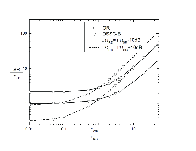
Figure 1: Relay switching rates of OR and DSSC

In this subsection, we illustrate some numerical results, regarding the relaying switching rate and average relaying activation time of both OR and DSSC-B. All the results were also confirmed by simulations. As already mentioned, the relay switching rate and the average relaying activation time constitute a vital part in the design and implementation of selective cooperative relaying, due to the complexity issues that each relay switching entails. Fig. 1 depicts the normalized switching rates of both OR and DSSC-B versus the ratio $\mathcal{F}_{SR_{i}}/\mathcal{F}_{R_{i}D}$ for $L=2$ relays, when the fading powers in the $S$-$R$ and $R$-$D$ links are unbalanced. Specifically, the average channel gains of the $S$-$R_{1}$ and $S$-$R_{2}$ links are assumed equal to each other, and the same is true for the $R_{1}$-$D$ and $R_{2}$-$D$ links; the difference in the corresponding average SNRs is 10dB, so that $\Gamma\Omega_{SR_{i}}=\Gamma\Omega_{R_{i}D}\pm 10$dB, $i\in\left\{1,2\right\}$. As observed from Fig. 1, the switching rate of DSSC-B is always smaller than that of OR, with the latter to be under specific conditions even ten times greater than the former. This verifies the intuition that DSSC-B leads to less frequent relay switchings, accounting thus for simpler practical implementations. It should be noted that in Fig. 1 the switching threshold, $T$, used is that threshold which leads to the maximum possible switching rate of DSSC-B, which is determined through numerical optimization methods. In other words, the DSSC-B curves depict the worst case in terms of switching rate, demonstrating that even in this scenario the DSSC-B switching rate is much less than that of OR.

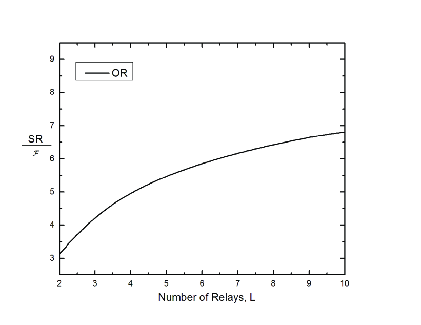
Figure 2: Relay switching rate of OR versus the number of available relays

The effect of the number of available relays on the switching rate of OR for the i.i.d. case with equal maximum Doppler frequencies in all of the links involved, is plotted in Fig. 2. As expected, the switching rate continuously increases as the number of the relays increases, yet in a non-linear manner. The main result extracted from Fig. 2 is that in cases where the number of available relays is large, leaving some of them out of the selection set may be preferable in practical applications with high Doppler spread, despite the apparent performance cost.

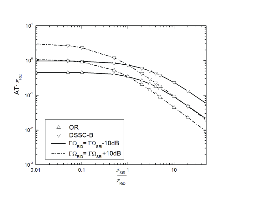
Figure 3: Average activation time of OR and DSSC

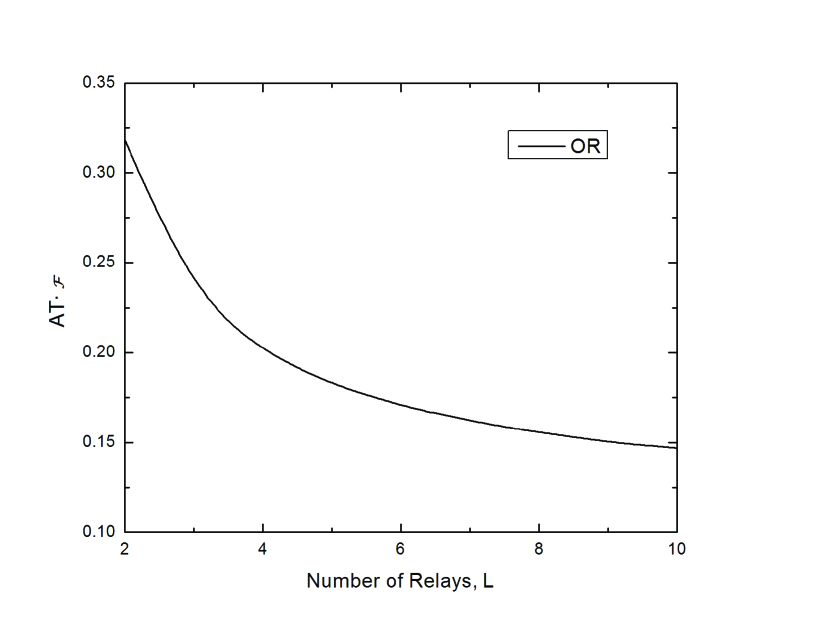
Figure 4: Average activation time of OR versus the number of available relays

The normalized average relay activation time of the relays for the same conditions as in Fig. 1 is plotted in Fig. 3. Again the average activation time in DSSC-B is the minimum possible, i.e., the parameter $T$ is properly selected so as to account for the worst case. Fig. 3 manifests that the average relay activation time of DSSC-B is considerably larger than that of OR, regardless of the assumptions on the relative $S$-$R$ and $R$-$D$ channel strengths. The effect of the number of relays on the activation time for OR is shown in Fig. 4. One may observe that the activation time reduces in a non-linear fashion as the number of relays reduces.

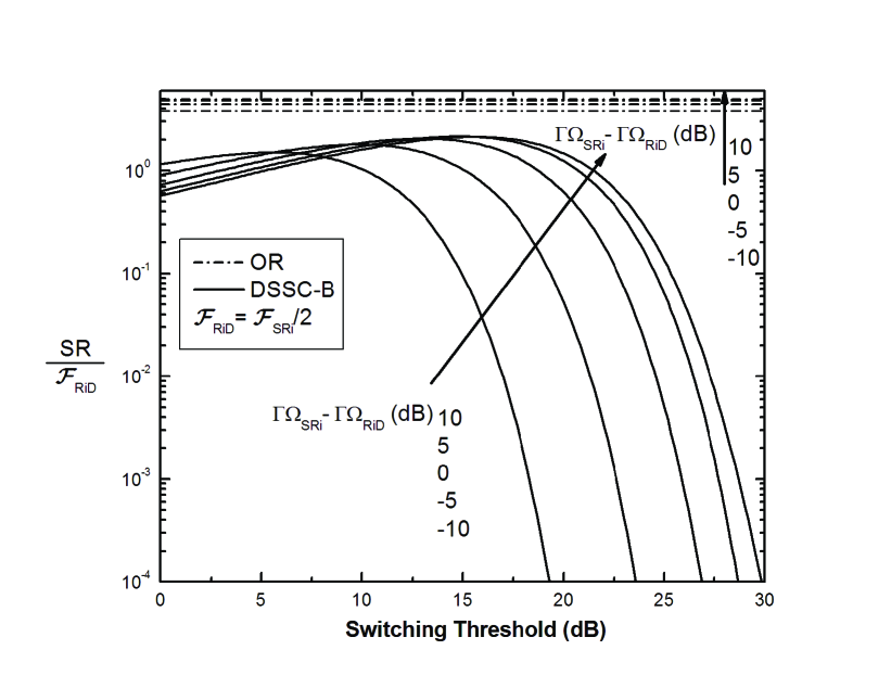
Figure 5: Relay switching rates of OR and DSSC versus the normalized switching threshold

Finally, in Fig. 5, the switching rates of OR and DSSC-B are plotted for $L=2$ relays and several values of the switching threshold, $T$, assuming that the channel gains in the $S$-$R$ and $R$-$D$ links are unbalanced, as well as that $\mathcal{F}_{SR_{i}}=2\mathcal{F}_{R_{i}D}$. For each of the scenarios shown here, the switching rate of DSSC-B is considerably lower than that of OR. The ratio of switching rates is, however, crucially dependent on the switching threshold of DSSC-B, implying that the difference of the switching rates of OR and DSSC-B shown in Fig. 1 is significantly expanded for $T$ values different from the worst (in terms of relay switching rate) case for DSSC-B.

VI Conclusion

We conducted a study of selective cooperative relaying in time-varying fading channels. In particular, we derived the relay switching rate for selective cooperative relaying, which reflects the concept of how frequently a cooperative scheme switches from one relay to another. Together with the relay switching rate, a closed-form expression for the average relay activation time was also derived, which corresponds to the average time which a relay remains activated until a switching occurs. Numerical results indicated that for the case where there are two relays available, selecting the active relay in a max SNR-based fashion (a.k.a. opportunistic relaying - OR) results in a considerably higher switching rate than selecting the relay in a DSSC-B fashion. Therefore, considering the complexity issues associated with frequent relay switching, DSSC-B leads to a simpler implementation of selective cooperative relaying than OR, and may be preferable in fast fading scenarios, despite being inferior in terms of error performance.

Appendix A

Evaluation of $f_{Z}\left(0\right)$

The PDF of $Z\left(t\right)$ evaluated at zero reflects the probability that the absolute difference of the virtual fading gains of the $S$-$R_{1}$-$D$ and $S$-$R_{2}$-$D$ channels lies in the infinitesimal interval $\left[0,dz\right]$. Therefore, $f_{Z}\left(0\right)$ can be expressed as

$$f_{Z}\left(0\right)=\int_{0}^{\infty}f_{a_{1}}\left(x\right)f_{a_{2}}\left(x\right)dx$$ (32)

where $f_{a_{1}}\left(\cdot\right)$ and $f_{a_{2}}\left(\cdot\right)$ denote the PDFs of the processes $a_{1}\left(t\right)$ and $a_{2}\left(t\right)$, respectively. Using (1) and (2), the CDF of $a_{i}\left(t\right)$, $i\in\left\{1,2\right\}$, is expressed as

$$F_{a_{i}}\left(x\right) =1-\int_{x}^{\infty}f_{SR_{i}}\left(\omega\right)d\omega\int_{x}^{\infty}f_{R_{i}D}\left(\omega\right)d\omega$$

$$=1-\exp\left(-\frac{\Omega_{SR_{i}}+\Omega_{R_{i}D}}{\Omega_{SR_{i}}\Omega_{R_{i}D}}x^{2}\right)$$ (33)

while the PDF of $a_{i}\left(t\right)$ is derived by differentiating (33), yielding

$$f_{a_{i}}\left(x\right)=2x\frac{\Omega_{SR_{i}}+\Omega_{R_{i}D}}{\Omega_{SR_{i}}\Omega_{R_{i}D}}\exp\left(-\frac{\Omega_{SR_{i}}+\Omega_{R_{i}D}}{\Omega_{SR_{i}}\Omega_{R_{i}D}}x^{2}\right).$$ (34)

Note that the process $a_{i}\left(t\right)$ is also Rayleigh distributed; its average squared value is denoted by $\Omega_{i}$ and is given by

$$\Omega_{i}=\frac{\Omega_{SR_{i}}\Omega_{R_{i}D}}{\Omega_{SR_{i}}+\Omega_{R_{i}D}}.$$ (35)

Then, $f_{Z}\left(0\right)$ is derived as the integral of the product of two Rayleigh distributions, yielding

$$f_{Z}\left(0\right)=\frac{4}{\Omega_{1}\Omega_{2}}\int_{0}^{\infty}x^{2}\exp\left(-\frac{\Omega_{1}+\Omega_{2}}{\Omega_{1}\Omega_{2}}x^{2}\right)dx.$$ (36)

Using [15, eq. (3.321.5)], (36) yields (12).

Appendix B

Derivation of $f_{\overset{\cdot}{Z}}\left(\cdot\right)$

The time derivative of $Z\left(t\right)$, $\overset{\cdot}{Z}\left(t\right)$, equals the difference of the time derivatives $\overset{\cdot}{a}_{1}\left(t\right)$ and $\overset{\cdot}{a}_{2}\left(t\right)$. Before proceeding in deriving $f_{\overset{\cdot}{Z}}\left(\overset{\cdot}{z}\right)$, we first obtain the PDF of $\overset{\cdot}{a}_{i}\left(t\right)$, $i\in\left\{1,2\right\}$, as

$$f_{\overset{\cdot}{a}_{i}}\left(x\right)=\Pr\left\{a_{SR_{i}}\leq a_{R_{i}D}\right\}f_{\overset{\cdot}{a}_{SR_{i}}}\left(x\right)+\Pr\left\{a_{SR_{i}}>a_{R_{i}D}\right\}f_{\overset{\cdot}{a}_{R_{i}D}}\left(x\right)$$ (37)

where $f_{\overset{\cdot}{a}_{SR_{i}}}\left(\cdot\right)$ and $f_{\overset{\cdot}{a}_{R_{i}D}}\left(\cdot\right)$ denote the PDF of the time derivatives of $a_{SR_{i}}$ and $a_{R_{i}D}$, respectively. Given that $a_{SR_{i}}$ and $a_{R_{i}D}$ are Rayleigh distributed, $f_{\overset{\cdot}{a}_{SR_{i}}}\left(\cdot\right)$ and $f_{\overset{\cdot}{a}_{R_{i}D}}\left(\cdot\right)$ can be expressed as [12]

$$f_{\overset{\cdot}{a}_{SR_{i}}}\left(x\right)=\frac{1}{\sqrt{2\pi}\overset{\cdot}{\sigma}_{SR_{i}}}\exp\left(-\frac{x^{2}}{2\overset{\cdot}{\sigma}_{SR_{i}}^{2}}\right)$$ (38)

$$f_{\overset{\cdot}{a}_{R_{i}D}}\left(x\right)=\frac{1}{\sqrt{2\pi}\overset{\cdot}{\sigma}_{R_{i}D}}\exp\left(-\frac{x^{2}}{2\overset{\cdot}{\sigma}_{R_{i}D}^{2}}\right)$$ (39)

i.e., $\overset{\cdot}{a}_{SR_{i}}$ and $\overset{\cdot}{a}_{R_{i}D}$ are zero-mean Gaussian random variables (RVs) with standard deviations $\overset{\cdot}{\sigma}_{SR_{i}}=\pi\mathcal{F}_{SR_{i}}\sqrt{\Omega_{SR_{i}}}$ and $\overset{\cdot}{\sigma}_{R_{i}D}=\pi\mathcal{F}_{R_{i}D}\sqrt{\Omega_{R_{i}D}}$, respectively. The steady-state probabilities $\Pr\left\{a_{SR_{i}}\leq a_{R_{i}D}\right\}$ and $\Pr\left\{a_{SR_{i}}>a_{R_{i}D}\right\}$ are given by

$$\Pr\left\{a_{SR_{i}}\leq a_{R_{i}D}\right\}=\int_{0}^{\infty}f_{a_{SR_{i}}}\left(x\right)\left[1-F_{a_{R_{i}D}}\left(x\right)\right]dx=\frac{\Omega_{R_{i}D}}{\Omega_{SR_{i}}+\Omega_{R_{i}D}}$$ (40)

$$\Pr\left\{a_{SR_{i}}>a_{R_{i}D}\right\}=\frac{\Omega_{SR_{i}}}{\Omega_{SR_{i}}+\Omega_{R_{i}D}}.$$ (41)

The PDF of $\overset{\cdot}{a}_{i}\left(t\right)$ is therefore derived as

$$f_{\overset{\cdot}{a}_{i}}\left(x\right)=\frac{1}{\sqrt{2}\pi^{3/2}\left(\Omega_{SR_{i}}+\Omega_{R_{i}D}\right)}\left[\frac{\Omega_{R_{i}D}\exp\left(-\frac{x^{2}}{2\pi^{2}\mathcal{F}_{SR_{i}}^{2}\Omega_{SR_{i}}}\right)}{\sqrt{\Omega_{SR_{i}}}\mathcal{F}_{SR_{i}}}+\frac{\Omega_{SR_{i}}\exp\left(-\frac{x^{2}}{2\pi^{2}\mathcal{F}_{R_{i}D}^{2}\Omega_{R_{i}D}}\right)}{\sqrt{\Omega_{R_{i}D}}\mathcal{F}_{R_{i}D}}\right]$$ (42)

where $i\in\left\{1,2\right\}$. Consequently, it follows from (9) that the PDF of the process $\overset{\cdot}{Z}\left(t\right)$ is expressed as [16, ch. 6]

$$f_{\overset{\cdot}{Z}}\left(x\right)=\int_{-\infty}^{\infty}f_{\overset{\cdot}{a}_{1}}\left(y+x\right)f_{\overset{\cdot}{a}_{2}}\left(y\right)dy.$$ (43)

Substituting (42) in (43) and making use of the integral [15, eq. (3.323.2)]

$$\int_{-\infty}^{\infty}\exp\left(-\frac{\left(y+x\right)^{2}}{\alpha_{1}}\right)\exp\left(-\frac{x^{2}}{\alpha_{2}}\right)dy=\sqrt{\pi\frac{\alpha_{1}\alpha_{2}}{\alpha_{1}+\alpha_{2}}}\exp\left(-\frac{x^{2}}{\alpha_{1}+\alpha_{2}}\right)$$ (44)

we derive the PDF of $\overset{\cdot}{Z}\left(t\right)$, $f_{\overset{\cdot}{Z}}\left(\cdot\right)$, as

$$f_{\overset{\cdot}{Z}}\left(x\right) =\frac{1}{\sqrt{2}\pi^{3/2}\left(\Omega_{SR_{1}}+\Omega_{R_{1}D}\right)\left(\Omega_{SR_{2}}+\Omega_{R_{2}D}\right)}\left[\frac{\Omega_{SR_{1}}\Omega_{SR_{2}}\exp\left(-\frac{x^{2}}{2\pi^{2}\left(\Omega_{R_{1}D}\mathcal{F}_{R_{1}D}^{2}+\Omega_{R_{2}D}\mathcal{F}_{R_{2}D}^{2}\right)}\right)}{\sqrt{\Omega_{R_{1}D}\mathcal{F}_{R_{1}D}^{2}+\Omega_{R_{2}D}\mathcal{F}_{R_{2}D}^{2}}}\right.$$

$$+\frac{\Omega_{R_{1}D}\Omega_{SR_{2}}\exp\left(-\frac{x^{2}}{2\pi^{2}\left(\Omega_{SR_{1}}\mathcal{F}_{SR_{1}}^{2}+\Omega_{R_{2}D}\mathcal{F}_{R_{2}D}^{2}\right)}\right)}{\sqrt{\Omega_{SR_{1}}\mathcal{F}_{SR_{1}}^{2}+\Omega_{R_{2}D}\mathcal{F}_{R_{2}D}^{2}}}+\frac{\Omega_{R_{2}D}\Omega_{SR_{1}}\exp\left(-\frac{x^{2}}{2\pi^{2}\left(\Omega_{SR_{2}}\mathcal{F}_{SR_{2}}^{2}+\Omega_{R_{1}D}\mathcal{F}_{R_{1}D}^{2}\right)}\right)}{\sqrt{\Omega_{SR_{2}}\mathcal{F}_{SR_{2}}^{2}+\Omega_{R_{1}D}\mathcal{F}_{R_{1}D}^{2}}}$$

$$+\left.\frac{\Omega_{R_{1}D}\Omega_{R_{2}D}\exp\left(-\frac{x^{2}}{2\pi^{2}\left(\Omega_{SR_{1}}\mathcal{F}_{SR_{1}}^{2}+\Omega_{SR_{2}}\mathcal{F}_{SR_{2}}^{2}\right)}\right)}{\sqrt{\Omega_{SR_{1}}\mathcal{F}_{SR_{1}}^{2}+\Omega_{SR_{2}}\mathcal{F}_{SR_{2}}^{2}}}\right].$$ (45)

Having an expression for $f_{\overset{\cdot}{Z}}\left(\cdot\right)$, the last term in (11) is derived using [15, eq. (3.321.4)] as shown in (13).

Appendix C

Relay Switching Rate of OR with $L$ available relays

Evaluation of $f_{Z}\left(0\right)$

Let us first derive the PDF of $a_{k}\left(t\right)$ as the PDF of the maximum of $L-1$ i.i.d. Rayleigh RVs, yielding

$$f_{a_{k}}\left(x\right)=\sum_{l=1}^{L-1}f_{a_{l}}\left(x\right)\prod_{\begin{subarray}{c}j=1\\ j\not=l\end{subarray}}^{L-1}F_{a_{j}}\left(x\right)=\left(L-1\right)f_{a}\left(x\right)\left[F_{a}\left(x\right)\right]^{L-2}$$ (46)

with $f_{a}\left(x\right)=\left(2x/\Omega\right)\exp\left(-x^{2}/\Omega\right)$ and $F_{a}\left(x\right)=1-\exp\left(-x^{2}/\Omega\right)$, where $\Omega=\Omega_{SR_{1}}/2=\Omega_{R_{1}D}/2=...=\Omega_{SR_{L}}/2=\Omega_{R_{L}D}/2$ denotes the average squared channel gain in each of the virtual end-to-end channels involved. Then, $f_{Z}\left(0\right)$ is derived as

$$f_{Z}\left(0\right)=\int_{0}^{\infty}f_{a}\left(x\right)f_{a_{k}}\left(x\right)dx=\left(L-1\right)\int_{0}^{\infty}f_{a}^{2}\left(x\right)\left[F_{a}\left(x\right)\right]^{L-2}dx\text{.}$$ (47)

Using the product expansion

$$\left[1-\exp\left(-\frac{x^{2}}{\Omega}\right)\right]^{L-2}=1+\sum_{l=1}^{L-2}\left(-1\right)^{l}\binom{L-2}{l}\exp\left(-l\frac{x^{2}}{\Omega}\right)$$ (48)

(47) yields

$$f_{Z}\left(0\right)=\frac{\left(L-1\right)\sqrt{\pi}}{\Omega^{2}}\sum_{l=0}^{L-2}\left(-1\right)^{l}\binom{L-2}{l}\left(\frac{\Omega}{l+2}\right)^{\frac{3}{2}}\text{.}$$ (49)

Derivation of $f_{\overset{\cdot}{Z}}\left(\cdot\right)$

Because of the i.i.d. assumption, the PDF of the time-derivative $\overset{\cdot}{a}_{i}\left(t\right)$ is derived from (42) as

$$f_{\overset{\cdot}{a}_{i}}\left(x\right)=\frac{1}{2\pi^{3/2}\mathcal{F}\sqrt{\Omega}}\exp\left(-\frac{x^{2}}{4\pi^{2}\mathcal{F}^{2}\Omega}\right)$$ (50)

that is, $\overset{\cdot}{a}_{i}$ is a zero-mean Gaussian RV with standard deviation $\overset{\cdot}{\sigma}_{a_{i}}=\pi\mathcal{F}\sqrt{\Omega}$. The PDF of the time-derivative of $a_{k}\left(t\right)$, $\overset{\cdot}{a}_{k}\left(t\right)$, is derived as

$$f_{\overset{\cdot}{a}_{k}}\left(x\right)=\sum_{j=1}^{L-1}\rho_{j}^{OR}f_{\overset{\cdot}{a}_{j}}\left(x\right)=f_{\overset{\cdot}{a}_{i}}\left(x\right)$$ (51)

which implies that, due to symmetry, the PDF of the time-derivative of the maximum of $L-1$ i.i.d. RVs, equals the PDF of each of the $L-1$ RVs. Using (43), the PDF of $\overset{\cdot}{Z}\left(t\right)=\overset{\cdot}{a}_{i}\left(t\right)-\overset{\cdot}{a}_{k}\left(t\right)$ is derived as

$$f_{\overset{\cdot}{Z}}\left(x\right)=\frac{1}{\left(2\pi\right)^{3/2}\mathcal{F}\sqrt{\Omega}}\exp\left(-\frac{x^{2}}{8\pi^{2}\mathcal{F}^{2}\Omega}\right).$$ (52)

Appendix D

Steady-State Relay Activation Probabilities of DSSC-B

Considering that relay switchings in DSSC-B are determined in exactly the same way as branch switchings in SSC-B, the steady-state relay activation probabilites for DSSC-B are derived through the Markov states of SSC-B given in [8]. Specifically, the Markov chain of DSSC-B yields six states, as follows. State 1 corresponds to the case where “$R_{1}$ is active and the overal SNR down-crosses $T$”; state 2 corresponds to “$R_{1}$ is active and the overall SNR is below $T$”; state 3 corresponds to “$R_{1}$ is active and the overall SNR is greater than $T$”; states 4, 5, 6 refer to the case where $R_{2}$ is active, and are defined analogous to 1, 2, 3, respectively. The stationary probabilities, $\pi_{j}^{DSSC-B},$ $j\in\left\{1,...,6\right\}$, of the above Markov states are taken from [8, eq. (21)], yielding

$$\pi_{1}^{DSSC-B} =\frac{\left[1-q_{1}\right]q_{1}\left[1-q_{2}\right]q_{2}}{\left[q_{1}+q_{2}\right]\left[1+2q_{1}q_{2}\right]-\left[q_{1}+q_{2}\right]^{2}-2q_{1}^{2}q_{2}^{2}}$$ (53a)

$$\pi_{2}^{DSSC-B} =\frac{q_{1}^{2}q_{2}\left[1-q_{2}\right]}{\left[q_{1}+q_{2}\right]\left[1+2q_{1}q_{2}\right]-\left[q_{1}+q_{2}\right]^{2}-2q_{1}^{2}q_{2}^{2}}$$ (53b)

$$\pi_{3}^{DSSC-B} =\frac{\left[1-q_{1}\right]^{2}\left[1-q_{2}\right]q_{2}}{\left[q_{1}+q_{2}\right]\left[1+2q_{1}q_{2}\right]-\left[q_{1}+q_{2}\right]^{2}-2q_{1}^{2}q_{2}^{2}}$$ (53c)

$$\pi_{4}^{DSSC-B} =\frac{\left[1-q_{1}\right]q_{1}\left[1-q_{2}\right]q_{2}^{2}}{\left[q_{1}+q_{2}\right]\left[1+2q_{1}q_{2}\right]-\left[q_{1}+q_{2}\right]^{2}-2q_{1}^{2}q_{2}^{2}}$$ (53d)

$$\pi_{5}^{DSSC-B} =\frac{q_{2}^{2}q_{1}\left[1-q_{1}\right]}{\left[q_{1}+q_{2}\right]\left[1+2q_{1}q_{2}\right]-\left[q_{1}+q_{2}\right]^{2}-2q_{1}^{2}q_{2}^{2}}$$ (53e)

$$\pi_{6}^{DSSC-B} =\frac{\left[1-q_{1}\right]q_{1}\left[1-q_{2}\right]q_{2}}{\left[q_{1}+q_{2}\right]\left[1+2q_{1}q_{2}\right]-\left[q_{1}+q_{2}\right]^{2}-2q_{1}^{2}q_{2}^{2}}$$ (53f)

where $$q_{1}=F_{a_{1}^{2}}\left(T/\Gamma\right) q_{2}=F_{a_{2}^{2}}\left(T/\Gamma\right) R_{1} R_{2} \rho_{1}^{DSSC}=\sum_{j=1}^{3}\pi_{j}^{DSSC-B} \rho_{2}^{DSSC}=\sum_{j=4}^{6}\pi_{j}^{DSSC-B}$$; . Considering that is active in the states 1, 2, 3, while in states 4, 5, 6, the steady-state relay activation probabilities of DSSC-B are derived as ; , yielding (27) and (28).

References

- [1] F. H. Fitzek and M. D. Katz, Cooperation in Wireless Networks: Principles and Applications, 1st ed. Dordrecht, Netherlands: Springer, 2007.
- [2] J. N. Laneman, D. N. C. Tse, and G. W. Wornell, “Cooperative diversity in wireless networks: Efficient protocols and outage behavior,” IEEE Trans. Inform. Theory, vol. 50, pp. 3062–3080, Dec. 2004.
- [3] Y. Zhao, R. Adve, and T. J. Lim, “Improving amplify-and-forward relay networks: optimal power allocation versus selection,” in Proc. IEEE Intern. Symp. Inform. Theory (ISIT 06), Seattle, WA, Jul. 2006.
- [4] A. Bletsas, A. Khisti, D. P. Reed, and A. Lippman, “A simple cooperative diversity method based on network path selection,” IEEE J. Selec. Areas Commun., vol. 24, pp. 659–672, Mar. 2006.
- [5] D. S. Michalopoulos and G. K. Karagiannidis, “Performance analysis of single relay selection in Rayleigh fading,” IEEE Trans. Wireless Commun., vol. 7, pp. 3718–3724, Oct. 2008.
- [6] R. Tannious and A. Nosratinia, “Spectrally efficient relay selection protocols in wireless networks,” in Proc IEEE Intern. Conf. on Acoustics, Speech and Signal Processing (ICASSP), Las Vegas, NV, Mar. 2008.
- [7] D. S. Michalopoulos and G. K. Karagiannidis, “Two relay distributed switch and stay combining (DSSC),” IEEE Trans. Commun., vol. 56, pp. 1790–1794, Nov. 2008.
- [8] H.-C. Yang and M.-S. Alouini, “Markov chains and performance comparison of switched diversity systems,” IEEE Trans. Commun., vol. 52, pp. 1113–1125, Jul. 2004.
- [9] P. A. Anghel and M. Kaveh, “Exact symbol error probability of a cooperative network in a Rayleigh-fading environment,” IEEE Trans. Wireless Commun., vol. 3, pp. 1416–1421, Sep. 2004.
- [10] S. Ikki and M. H. Ahmed, “Performance analysis of cooperative diversity wireless networks over Nakagami- fading channel,” IEEE Communications Letters, vol. 11, pp. 334–336, Apr. 2007.
- [11] P. S. Bullen, D. S. Mitrinovic, and P. M. Vasic, Means and their Inequalities. Dordrecht: Kluwer Academic Publishers, 1988.
- [12] S. Rice, “Statistical properties of a sine wave plus noise,” Bell Syst. Tech. J., vol. 27, pp. 109–157, Jan. 1948.
- [13] N. C. Beaulieu, “Switching rates of dual selection diversity and dual switch-and-stay diversity,” IEEE Trans. Commun., vol. 56, pp. 1409–1413, Sep. 2008.
- [14] F. Sivrikaya and B. Yener, “Time synchronization in sensor networks: A survey,” IEEE Network J., vol. 18, pp. 45–50, Jul. 2004.
- [15] I. S. Gradshteyn and I. M. Ryzhik, Table of Integrals, Series, and Products, 6th ed. New York: Academic, 2000.
- [16] A. Papoulis, Probability, Random Variables, and Stochastic Procceses, 3rd ed. McGraw-Hill, 1991.