The Fifth Data Release Sloan Digital Sky Survey/XMM-Newton Quasar Survey

Abstract

We present a catalog of 792 DR5 SDSS quasars with optical spectra that have been observed serendipitously in the X-rays with the XMM-Newton. These quasars cover a redshift range of z = 0.11 - 5.41 and a magnitude range of $i$ = 15.3-20.7. Substantial numbers of radio-loud (70) and broad absorption line (51) quasars exist within this sample. Significant X-ray detections at $\geq 2\sigma$ account for 87% of the sample (685 quasars), and 473 quasars are detected at $\geq$ 6$\sigma$, sufficient to allow X-ray spectral fits. For detected sources, $\sim$ 60% have X-ray fluxes between F_2-10keV = 1 - 10 x 10^-14 ergs cm^-2 s^-1. We fit a single power-law, a fixed power-law with intrinsic absorption left free to vary, and an absorbed power-law model to all quasars with X-ray S/N $\geq$ 6, resulting in a weighted mean photon index $\Gamma$ = 1.91$\pm$0.08, with an intrinsic dispersion $\sigma_{\Gamma}$ = 0.38. For the 55 sources (11.6%) that prefer intrinsic absorption, we find a weighted mean N_H = 1.5$\pm$0.3 x 10²¹ cm^-2. We find that $\Gamma$ correlates significantly with optical color, $\Delta$($g-i$), the optical-to-X-ray spectral index ($\alpha_{ox}$) and the X-ray luminosity. While the first two correlations can be explained as artefacts of undetected intrinsic absorption, the correlation between $\Gamma$ and X-ray luminosity appears to be a real physical correlation, indicating a pivot in the X-ray slope.

1 Introduction

Catalogs are indispensable in performing statistical studies of quasar properties. The known correlations between optical and X-ray properties, discussed further below, imply a connection between the accretion disk posited to feed the central black hole (Shakura & Sunyaev, 1973) and the hot Compton-scattering corona posited to lie in some unknown geometry around the disk (Haardt & Maraschi, 1991). While quasars were first discovered in early radio surveys (e.g. 3C, 3CR, PKS, 4C, AO), most quasar surveys since then have been conducted in the optical/UV. Early quasar selection techniques included UV-excess selection and emission line searches using slitless spectroscopy.

UV-excess selection utilizes the Big Blue Bump that dominates the optical/UV spectrum to distinguish quasars from stars. The Big Blue Bump is normally attributed to a multi-temperature accretion disk (Shields et al., 1978; Malkan & Sargent, 1982). UV-excess based surveys include the Braccesi et al. (1970) catalog, which contains 175 objects with U - B $<$ -0.42, and the Palomar-Green (PG) Bright Quasar Survey (BQS, Schmidt & Green, 1983), a sample of 92 objects selected with U - B $<$ -0.44. Slitless spectroscopy, with prisms or grisms, obtains a large number of low-resolution spectra for a single field. For example, the objective prism on the Curtis Schmidt telescope at CTIO found 174 confirmed quasars, ranging in redshift from z = 0.1 to z = 3.3 (Osmer & Smith, 1980; Osmer, 1981). Slitless spectroscopy often incorporated UV-excess selection as well; the primary example of this technique is the Markarian survey (Markarian, 1967; Markarian et al., 1981), which searched for galaxies with unusually blue continua using a grism. The Large Bright Quasar Survey (LBQS; Hewett et al. 1995) used a combination of color selection and the presence of emission features on objective prism plates to obtain a homogenous sample of 1055 quasars spanning a wide redshift range (0.2 $\leq$ z $\leq$ 3.4).

However, both of these techniques suffer from serious biases. While slitless spectroscopy has a high selection efficiency, even at higher redshifts, it is biased against quasars with weak emission lines, and cannot reach as faint a flux limit. The UV-excess selection method is biased against ”red” sources, where red colors may be due to high-redshift (the Ly$\alpha$ line enters the spectrum at z $\sim$ 2), dust-reddening, significant host galaxy contribution, or intrinsically red emission mechanisms. With the advent of the ‘UK Schmidt Survey’ (Warren et al., 1991), the Two-Degree Field (2DF; Croom et al., 2001) and the Sloan Digital Sky Survey (SDSS; York et al. 2000) quasar catalogs, multicolor selection techniques that used up to 5 photometric bands were introduced that could select red quasars in addition to blue ones, provided the sources were within the survey flux limit. The 5th Data Release (DR5) SDSS quasar catalog has surpassed all previous optical surveys by providing high quality photometry and spectroscopy for 77,429 quasars (Schneider et al., 2007) spanning redshifts from z = 0.08 to z = 5.41.

As quasars emit strongly over eight decades of the spectrum (e.g. Elvis et al., 1994), multiwavelength surveys are necessary to relate the optical/UV accretion emission to other components, notably the non-thermal emission seen in the X-rays. However, X-ray spectra are time-consuming and expensive to obtain for large samples. For this reason, previous studies of optical and X-ray correlations consist largely of two types: (1) Small samples (N $\sim$ 20-50) with detailed X-ray spectral analysis have been compiled by observing sub-samples of optical surveys with X-ray telescopes (e.g. Laor et al., 1997; Elvis et al., 1994; Piconcelli et al., 2005; Shemmer et al., 2006, 2008). The Akylas et al. (2004) XMM-Newton/2dF survey is larger, with 96 2QZ quasars observed in wide field (2.5 deg²), shallow (2-10 ks per pointing, f(0.5-8 keV) $\sim$ 10^-14 erg cm^-2 s^-1) XMM observations. (2) Still larger samples (N $\sim$ 200-300) with only X-ray fluxes have been compiled for statistical investigations. These larger studies have to assume an X-ray spectral slope (e.g. Vignali et al., 2003; Strateva et al., 2005; Steffen et al., 2006).

The ever-expanding archive of X-ray observations now provides a less costly and time-consuming method of obtaining X-ray spectra for large numbers of optically-selected quasars. Kelly et al. (2007) cross-correlated the SDSS DR3 quasar catalog with archival Chandra observations (Weisskopf, 1991) to obtain 174 quasars, 44 of which have sufficient counts to fit an absorbed power-law with $\Gamma$ and N_H as free parameters. This sample was extended to a total of 318 quasars (Kelly et al., 2008) by adding 149 RQ objects from an SDSS-ROSAT cross-correlation (Strateva et al., 2005). As only single power-law models were fit to the ROSAT spectra with sufficient counts, 153 of 318 sources have X-ray spectra slopes, but no fits for intrinsic absorption were made. Archival Chandra observations have also been used to identify an X-ray-selected AGN population in the Chandra Multiwavelength Project (Green et al., 2003). In addition, a large sample (N = 1135) of optically selected SDSS quasars with photometric redshifts are detected in the X-rays in Chandra fields (Green et al., 2008), of which 156 have sufficient counts ($>200$) to fit an absorbed power-law with $\Gamma$ and N_H as free parameters.

XMM-Newton is a good choice for cross-correlating with optical catalogs due to its large field of view and large effective area. Images are made with the three European Photon Imaging Cameras (EPIC): MOS-1 and MOS-2 (Turner et al., 2001), each of which has a 33’ x 33’ field of view, and the pn camera (Strueder et al., 2001), which has a 27.5’ x 27.5’ field of view.. XMM’s large effective area (922 cm² for MOS and 1,227 cm² for PN at 1 keV)⁴ results in higher signal-to-noise X-ray spectra than with Chandra for bright, non-background-limited sources. The EPIC CCDs have good spectral resolution (E/$\Delta$E $\sim$ 20 - 50 for both MOS and PN) over the 0.5 - 10 keV band.

Archival XMM-Newton observations overlapped with $\sim$1% of the SDSS DR5 coverage as of Feb. 2007. The SDSS and XMM-Newton archives are well-matched in sensitivity, as discussed in Young et al. (2008). The 5th Data Release (DR5, Adelman-McCarthy et al., 2007) of the SDSS covers a spectroscopic area of 5740 deg², and contains 90,611 quasars. The SDSS photometry in the $u$, $g$, $r$, $i$ and $z$ bands covers 3,250 - 10,000 Å, while the spectroscopy covers 3,800 - 9,200 Å with a spectral resolving power of $\sim$ 2,000. The SDSS is $\sim$95% complete for point sources to a limiting magnitude $i=19.1$, corrected for Galactic reddening (Richards et al., 2002; Vanden Berk et al., 2005).

A preliminary cross-correlation of DR1 SDSS quasars with the XMM-Newton public archive yielded 55 objects with exposure times greater than 20 ks (Risaliti et al., 2005). Of these, 35 yielded good X-ray spectra. Risaliti et al. (2005) estimated that a cross-correlation of a final SDSS data release with the ever-growing XMM-Newton archive would yield $\sim$ 1000 quasars, of which $\sim$80% would have good X-ray spectra.

In this paper, we cross-correlate the SDSS DR5 quasar catalog with archival XMM-Newton observations to obtain a large (N$\sim$800) sample of quasars with X-ray detections, almost 500 of which have good optical and X-ray spectral data. Below, we outline two immediate goals for the SDSS/XMM-Newton Quasar Survey: (1) to conduct large, statistical studies to understand the physical basis behind optical/X-ray correlations and (2) to investigate interesting sub-populations of quasars.

1.1 Optical/X-ray Correlations

The relations between optical and X-ray continuum and spectral properties promise to reveal clues about the disk-corona structure of quasars. The large sample provided by the SDSS/XMM-Newton Quasar Survey allow two correlations to be investigated. The first of these is the controversial $\alpha_{ox}-l_{2500\AA}$ relation: many studies have found that the spectral index from 2500 Å to 2 keV, defined as $\alpha_{ox}$ = log(L_2keV/ L₂₅₀₀)/log($\nu_{2keV}$/$\nu_{2500}$), anti-correlates with the log of the monochromatic luminosity at 2500 Å, $l_{2500\AA}$ (Tananbaum et al., 1979; Zamorani et al., 1981; Avni & Tananbaum, 1982; Kriss & Canizares, 1985; Tananbaum et al., 1986; Anderson & Margon, 1987; Wilkes et al., 1994; Pickering et al., 1994; Avni, Worrall & Margon, 1995; Vignali et al., 2003; Strateva et al., 2005; Shen et al., 2006; Steffen et al., 2006; Just et al., 2007). However, some studies (Bechtold et al., 2003; Kelly et al., 2007) find the primary relation to be between $\alpha_{ox}$ and redshift, while other studies (Yuan et al., 1998; Tang et al., 2007) find that the correlation may be induced by selection effects.

No physical basis for the $\alpha_{ox}-l_{2500\AA}$ relation has yet been proposed, and the relation itself provides little guidance. In part, this is because previous studies have largely used the traditional, observationally convenient, but physically arbitrary, endpoints of 2500 Å and 2 keV. They also assume an X-ray photon index ($\Gamma\sim$ 2, where $\Gamma$ = -$\alpha$ + 1 for F${}_{\nu}\propto\nu^{\alpha}$) to obtain the X-ray flux at 2 keV. A systematic study with measured optical and X-ray spectra would enable an investigation of the relation at different frequencies than those traditionally used, hopefully revealing clues about the relation’s physical underpinnings (Young et al. 2009b, in prep.).

The second correlation is the positive relation between $\Gamma$ and the normalized accretion rate, L/L_Edd (Shemmer et al., 2006, 2008). While early studies focused on the relation between $\Gamma$ and full-width half-maximum of the H$\beta$ line, FWHM(H$\beta$) (Boller et al., 1996; Laor et al., 1997; Brandt et al., 1997), Shemmer et al. (2006, 2008) have broken the degeneracy between FWHM(H$\beta$) and L/L_Edd by including highly luminous sources in order to show that $\Gamma$ depends primarily on L/L_Edd. There have been suggestions that this dependence may be due to the disk emitting more and softer photons as accretion rates increase, leading to more efficient Compton cooling in the corona (Laor, 2000; Kawaguchi et al., 2001).

Until now, studies of the $\Gamma$-L/L_Edd relation have consisted of small samples (N $\sim$ 40). The SDSS/XMM-Newton quasar survey can increase this sample size by an order of magnitude, leading to a better defined relation (Risaliti et al. 2009, in prep.).

1.2 Quasar Sub-Populations

Interesting quasar sub-populations can be readily investigated due to the large number of sources in the SDSS/XMM-Newton Quasar Survey. For example, red quasars make up 6% of the SDSS sample (Richards et al., 2003). Their steep optical slopes have been attributed to dust-reddening (Richards et al., 2003; Hopkins et al., 2004), though observations of individual objects suggest that some slopes may be intrinsically steep (Risaliti et al., 2003; Hall et al., 2006). In Young et al. (2008), we studied 17 quasars with extreme red colors ($g-r>0.5$) and moderate redshifts (1 $<$ z $<$ 2). By using X-ray observations in conjunction with optical spectra, we constrained the amount of intrinsic absorption in each source, thereby allowing the separation of intrinsically red from dust-reddened optical continua. We find that almost half (7 of 17) of the quasars can be classified as probable ‘intrinsically red’ objects. These quasars have unusually broad MgII emission lines ($<$FWHM$>$=10,500 km s^-1), flat but unabsorbed X-ray spectra ($<\Gamma>$ = 1.66$\pm$0.08), and low accretion rates ($\dot{M}/\dot{M_{Edd}}\sim$ 0.01).

Other interesting sub-populations for future investigations include broad absorption line (BAL), Type 2, and radio-loud (RL) quasars.

In this paper, we describe the SDSS quasar selection and the method with which we match sources to XMM-Newton observations in §2. X-ray data reduction is described in §3 and the resulting sample and correlations are discussed in §4. We assume a standard cosmology throughout the paper, where H₀ = 70 km s^-1 Mpc^-1, $\Omega_{M}=0.3$, and $\Omega_{\Lambda}=0.7$ (Spergel et al., 2003).

2 Data

2.1 SDSS Quasar Selection

As the DR5 quasar catalog (Schneider et al., 2007) was not yet available at the time of selection, we selected quasars with optical spectra directly from the DR5 SDSS database by choosing SpecClass = 3 (QSO) or 4 (QSO with z $>$ 2.3, whose redshift has been confirmed using a Ly$\alpha$ estimator). These quasars were selected for spectroscopic follow-up by the SDSS primarily due to their photometric colors, although some quasars were selected because they have a match in the FIRST survey (White et al., 1997). No X-ray selection is involved. Target selection efficiency, i.e. the percentage of sources spectroscopically observed that are confirmed as quasars, is 66% (Richards et al., 2002; Vanden Berk et al., 2005). The selection method is described in detail by Richards et al. (2002), and is summarized briefly below.

The vast majority ($\sim$95%) of SDSS quasar candidates are detected using a multicolor selection technique. Quasar candidates are defined to be any object at least 4$\sigma$ away from the stellar locus, which is defined in the ($u-g$,$g-r$,$r-i$,$i-z$) color space. In addition, special color-color regions are defined to specifically include or exclude quasar candidates. Inclusion regions include quasar candidates from 2.5 $<$ z $<$ 3, even if their colors cross the stellar locus. Exclusion regions prevent contamination due to white dwarfs, A stars and M star-white dwarf pairs.

For both radio and color-selected quasar candidates, magnitude limits are applied. Quasar candidates brighter than $i$ = 15 are rejected for spectroscopic follow-up because bright sources can contaminate the spectra of objects in adjacent fibers in the SDSS spectograph. Radio and low-redshift color-selected candidates fainter than $i$ = 19.1, which have a high number density on the sky, are also rejected due to the limited number of optical fibers for follow-up spectroscopy. Since high redshift (z $\gtrsim$ 3) quasar candidates have a lower surface density on the sky, a fainter cut-off magnitude $i$ = 20.2 is applied to these objects.

SDSS selected a small number of quasar candidates ($\sim$5%) by matching point sources with the position of a radio detection from the FIRST survey to within 2”. While the DR5 quasar catalog (Schneider et al., 2007) includes sources selected by matching to ROSAT detections, the initial SDSS quasar selection outlined in Richards et al. (2002) does not use X-ray detection as a criterion.

While SDSS radio selection requires that a source be point-like, their color selection includes extended sources as well, in order to include low-redshift AGN, such as Seyfert galaxies. However, in addition to having colors distinct from the stellar locus, extended sources must also have colors distinct from the main galaxy distribution. (The main galaxy distribution overlaps the stellar locus; however, a galaxy can be a clear outlier from the stellar locus both due to the shape of the stellar locus and because the stellar locus is determined primarily from F and M stars that dominate the Galactic stellar density at high latitudes.) Simple color cuts are applied to distinguish extended sources from galaxies, rather than an additional multicolor selection.

The DR5 quasar catalog (Schneider et al., 2007) additionally requires: luminosities brighter than M_i = -22.0; at least one emission line with a FWHM greater than 1000 km s^-1 or interesting/complex absorption features; magnitudes fainter than i = 15.0; and highly reliable redshifts. This results in a catalog of 77,429 quasars. We used only those quasars that are also in the DR5 Quasar Catalog for further analysis. Of the 92 sources we reject from our sample, $\sim$40% are Type 2 quasars. These will be the subject of a later study.

We matched The selected SDSS quasars with the FIRST survey (White et al., 1997) using a search radius of 3” in order to calculate their radio-loudness (R_L = F_5GHz / F₄₄₀₀, Kellerman et al. 1989)). A source is taken to be radio loud (RL) if R${}_{L}>$ 10. A power-law is interpolated between the optical magnitudes to get F_λ(4400Å), and the 1.4 GHz radio flux is obtained from FIRST survey detections, which are extrapolated to 5 GHz using a radio power-law $\alpha_{R}$ = -0.8. All the quasars lie in the area covered by the FIRST survey, so if there is no detection, we use the 5$\sigma$ upper-limit on the 1.4 GHz radio flux to extrapolate to 5 GHz. For 40 quasars, the upper-limit is too high to determine whether the source is radio-loud. Of the remaining quasars, 70 (9.3%) are radio-loud and 682 (90.7%) are radio-quiet, a typical ratio (e.g. Kembhavi & Narlikar 1999, pp. 256-263).

The SDSS color-color selection is effective at finding a variety of Broad Absorption Line (BAL) quasars (Schneider et al., 2007). The official DR5 BAL catalog (Gibson et al., 2009) had not yet been published during the writing of this paper, so we used an incomplete list of $\sim$ 4200 BALs in the DR5 Quasar Catalog (Shen et al., 2008a), selected using traditional criteria (Weymann et al., 1991). Using Shen et al. (2008a), we find 52 BALs in the SDSS-XMM Quasar Survey. Of these, 15 BALs have high enough X-ray signal-to-noise to obtain X-ray spectra (see §3). Since BALs are normally identified by CIV absorption features, which are visible only above a redshift z = 1.6 in SDSS spectra, BALs are unlikely to be identified in $\sim$56% of the SDSS-XMM quasars. BALs make up 14.5% of the SDSS/XMM quasars with z $>$ 1.6, which is in line with the parent population in Shen et al. (2008a).

In this paper, we measure the optical color of a quasar by its relative color (Richards et al., 2003). Relative colors compare a quasar’s measured colors with the median colors in its redshift bin, where redshift bin sizes are 0.1 in redshift, so that $\Delta$($g-i$) = ($g-i$) - $<$($g-i$)$>_{z}$. The use of relative colors corrects for the effect of typical emission lines on the photometry in a particular band. The relative ($g-i$) colors of the SDSS quasars match a Gaussian distribution on the blue side but require the addition of a tail on the red side [see Fig. 3 in Richards et al. (2003)].

2.2 Matching with the XMM-Newton Archive

We matched the SDSS quasars with the XMM-Newton archive from February 2007, choosing only those quasars that fell within 14’ of XMM observation field centers (typically 2-3 quasars per field). As part of the extraction process, described below, a source region is defined around each set of SDSS quasar coordinates. Depending on the S/N of the source, the extraction radius can range from 10 - 85”, with a typical radius of 19”. Low S/N objects are extracted with smaller radii to minimize the effect of high background levels, while larger radii for high S/N objects allow for an increased encircled energy fraction in the presence of relatively low background levels. The large extraction radii take into account the XMM point spread function (PSF), which is characterized by the radius at which 90% of the total energy is encircled. This radius increases from 48” (MOS) and 51.5” (PN) at 0’ off-axis angle to 52.5” (MOS) and 66” (PN) at 12’ off-axis angle. The extraction radii also take positional accuracy into account: SDSS positional errors are negligible (0.1” at the survey limit of r=22 for typical seeing, Pier et al. 2003), while the XMM positional accuracy is 3” at 3$\sigma$ for offset angles 0 $<\theta<$ 10 arcmin and 6” for 5 $<\theta<$ 10 arcmin (Pierre et al., 2007).

Multiple X-ray observations exist for 265 sources. In these cases, all observations were retrieved and reduced, but only the observation with the longest exposure time was used for further analysis. To avoid biases, we did not select the highest S/N observations, although in $\sim$80% cases, the two selections would be effectively the same.

The chance of including an unrelated random source within the extraction region is small but non-zero. Within a $\sim$14’ radius field of view, and using the average extraction radius, 19”, there are 1954 “beams” in an observation. Since there are $\sim$70 sources in a typical XMM observation (Watson et al., 2008, which has an exposure time distribution similar to that in this paper), this results in a 3.6% chance of extracting a random source rather than the SDSS-selected quasar. Since a random source is likely to be faint in the X-rays, any contamination is only significant for sources under 100 net counts. We have 792 unique sources, of which 390 have less than 100 net counts, so $\sim$14 (2% of the SDSS/XMM quasar sample) have significant contamination from an unrelated ‘interloper’ source.

2.3 X-ray Data Reduction

The 582 X-ray observations were processed using the XMM-Newton Science Analysis System, SAS v7.02. We reprocessed the events to ensure that each observation has the same, up-to-date calibration, and then filtered the observations to remove time intervals of flaring high-energy background events using the standard cut-off of 0.35 cts s^-1 for the MOS cameras and 1.0 ct s^-1 for the PN camera. Source and background regions were defined in a semi-automatic process. The SAS task eregionanalyse was used to optimize the source extraction radius for signal-to-noise. Most radii include at least 80% of the source counts. Background regions were defined by eye, avoiding obvious X-ray sources and chip edges. These regions were typically a circle of radius 2000-2500 pixels (100-125”), selected to lie at the same off-axis angle as the source and as close to the source as possible without overlapping the source extraction region. Once source and background regions were defined for every SDSS quasar in an observation, spectra were extracted for a total of 1380 non-unique quasars in 582 observations.

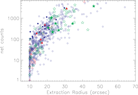
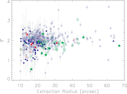
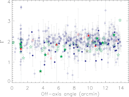
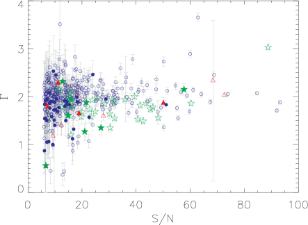
Figure 1: (a) Net counts vs. source extraction radius (arcseconds). (b) $\Gamma$ vs. source extraction radius. (c) X-ray photon index ($\Gamma$) vs. off-axis angle (arcmin). (d) $\Gamma$ vs. S/N.

To check for biases in the data reduction, Figures 1$a-b$ show the net counts and the X-ray photon index ($\Gamma$) plotted against the extraction radius. Figures 1$c-d$ plot the off-axis angle and the X-ray S/N against $\Gamma$. In Fig. 1$a$, the net counts are expected to correlate with the extraction radius, since the extraction radius will increase to larger encircled energy fraction for sources that stand higher above the background. The lack of correlations in Fig. 1$b$-$c$ show that the encircled energy correction takes the extraction radius and off-axis angle into account correctly. Fig 1$d$ shows that objects with flat $\Gamma$ are primarily found among low S/N objects, where absorption may be undetected in a spectral fit.

Where possible, observations were processed for all three XMM EPIC CCDs. In $\sim$40% of the observations, a source lies in a bad region in one or two of the three cameras, either in a strip between two chips or, because the MOS and PN cameras have different shapes, outside the field of view in one of the cameras. In these cases, we use the remaining images from the other cameras for analysis.

Table 1 contains observational data for each quasar in the DR5 SDSS/XMM- Newton Survey: the SDSS name, XMM observation ID, redshift, Galactic column density in the direction of the source, X-ray signal-to-noise, observation exposure time, off-axis angle, net source counts, background counts (from a background region that is scaled to the area of the source region), and two flags indicating if a source is RL or BAL.

Figure 2 summarizes the survey characteristics. The X-ray exposure times (Fig. 2$a$) range from 1.6 to 294 kiloseconds, though the majority of observations lie between 20 and 100 kiloseconds. This range in exposure times results in a wide range in sensitivity. While most sources have low signal-to-noise, a significant fraction have S/N $\geq$ 10, where more complex models can be fit (Fig. 2$b$). The detection fraction is $\gtrsim$ 80% until z $>$ 3.5 (Fig. 2$c$), but spectral coverage drops off fairly quickly for sources with z $>$ 2 (Fig. 2$d$).

3 X-ray Analysis: Spectral Fits

We made fits to the extracted spectra using the Sherpa package within CIAO. For each source, the available MOS+PN spectra were fit simultaneously over the 0.5 - 10 keV band. The observations were fit according to their S/N, with more complicated models being applied as S/N increased. All the models included local absorption fixed to the Galactic hydrogen column density (N_H,gal) at each source location. Values for N_H,gal were taken from the N_H tool available at WebPIMMS, which is based on the 21 cm HI compilation of Dickey & Lockman (1990) and Kalberla et al. (2005).

For the 319 low S/N sources (S/N $\leq$ 6), we fix a power-law to the weighted mean obtained for the high S/N (S/N $\geq$ 6) quasars in the sample, $\Gamma\sim$ 1.9 (§4.1), and allow only the normalization to vary in order to obtain the flux. For the 101 sources with S/N $<$ 2, we obtain a 90% upper-limit to the flux. We use the Cash (1979) statistic, which gives more reliable results for low-count sources, to fit sources with S/N $\leq$ 6. As the background is not subtracted and is instead fit simultaneously with the source, we apply a background model with three components, as described in Lumb et al. (2002) and in the XMM Users’ Handbook: a power-law (for the extragalactic X-ray spectrum), a broken power-law (for the quiescent soft proton spectrum), and two spectral lines (for cosmic-ray interactions with the detector). All parameters except for the normalization of the spectral lines were fixed. For 13 undetected sources, and 5 detected sources, this fit results in bad or null flux values. In these cases, we flag the source as undetected (flag = -1 in column (9) of Table 2) and we list the $\alpha_{ox}$ values as 9.99 (column (8) of same table).

For the 473 sources with enough S/N to fit spectral parameters (S/N $\geq$ 6), we use the $\chi^{2}$ statistic to fit three models: a single power-law (SPL) with no intrinisc absorption, a fixed power-law (FPL) where intrinsic absorption is left free to vary, and an intrinsically absorbed power-law (APL). The F-test, which measures the significance of the change in $\chi^{2}$ as components are added to a model, is used to determine whether the data prefer the APL model. To compare the SPL and FPL models, we simply compare the respective $\chi^{2}_{\nu}$ values, since both models have the same number of parameters. Therefore, the best-fit model is the one preferred by the F-test that also has the lowest $\chi^{2}_{\nu}$ value.

For sources with an unacceptable $\chi^{2}_{\nu}$ values for all three models, we by default make the SPL model the best-fit, but we also list the APL 90% upper-limit on intrinsic absorption. We plot the reduced $\chi^{2}$ distribution in Figure 3. A later paper will look in more detail at sources with bad fits ($\chi_{\nu}^{2}>1.2$).

Results for the best-fit models are listed in Table 2, including observed-frame and rest-frame fluxes (or 90% upper-limits), $\alpha_{ox}$, a flag indicating the best-fit X-ray spectral model, the photon index, intrinsic absorption (or 90% upper-limit) and the $\chi^{2}$ values and degrees of freedom for the best-fit model. The best-fit flag indicates which values are listed for each best-fit model. For sources that prefer the APL model (flag = 3), both $\Gamma$ and N_H are from the APL fit. If the FPL model is preferred (flag = 2), the SPL $\Gamma$ and FPL N_H are listed. For sources that prefer the SPL model (flag = 1), $\Gamma$ is from the SPL fit and N_H is the 90% upper-limit from the APL fit.

4 Results and Discussion

The SDSS/XMM-Newton Quasar Survey contains 792 sources, 685 of which are detected in the X-rays and 473 of which have X-ray spectra. (All have optical spectra.) The catalog covers redshifts z = 0.11 - 5.41 and optical magnitudes range from $i$ = 15.3 to $i$ = 20.7. Figures 4 shows the survey sensitivity in the optical ($a$) and X-ray ($b$) bands, and the observed-frame 2-10 keV flux distribution ($c$). The FWHM of the distribution spans F_2-10keV = (1 - 10) x 10^-14 ergs cm^-2 s^-1 and contains $\sim$ 60% of the detected sources.

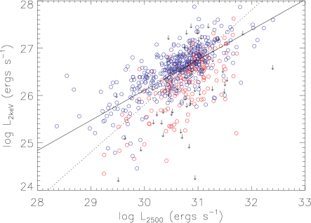
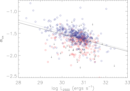
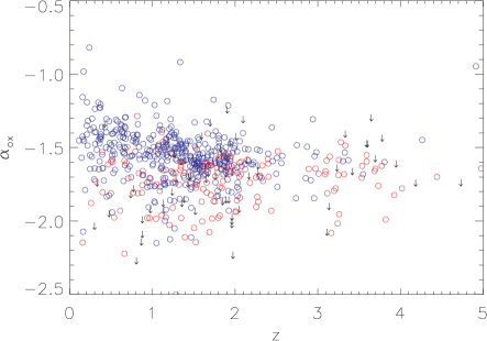
Figure 5: (a) $l_{2keV}$ vs. $l_{2500}$. The dotted line shows $l_{2keV}\propto l_{2500}$, constrained to pass through the average values of $l_{2keV}$ and $l_{2500}$. (b) The $\alpha_{ox}-l_{2500}$ relation for the SDSS/XMM quasar sample. The linear fit to the SDSS/XMM sample is plotted as a solid line, and the Steffen et al. line is overplotted as a dotted line for comparison. (c) $\alpha_{ox}$ vs. redshift. Red circles represent detected sources with X-ray S/N $<$ 6, and blue circles represent sources with X-ray S/N $>$ 6. BALs and RL quasars were removed from all three plots.

Results of standard $\alpha_{ox}$ analysis (i.e. using the conventional 2500 Å and 2 keV fiducial points) are shown in Figure 5. We test for correlations with $\alpha_{ox}$ using the Kendall correlation test available in ASURV, a survival statistics package (Lavalley et al., 1992). Figure 5$a$ shows log L_2keV vs. log L₂₅₀₀ with a dotted line of slope unity for reference. The best-fit line, obtained from the EM (estimate and maximize) algorithm within ASURV, is flatter than unity with a slope of 0.64 $\pm$ 0.03. This deviation from unity is clear in Figure 5$b$, which shows the $\alpha_{ox}-l_{2500\AA}$ correlation, significant at the 11.4$\sigma$ level in the SDSS/XMM Quasar Survey. The solid line is the best-fit EM regression line for our data:

$$\alpha_{ox}=(3.080\pm 0.376)+(-0.153\pm 0.012)log(L_{2500\AA})$$

The slope is consistent within errors with the best-fit regression from Steffen et al. (2006) (dotted line in Fig. 5b).

Figure 5$c$ plots $\alpha_{ox}$ against redshift. We find no correlation between $\alpha_{ox}$ and redshift, as in R05. The lack of an $\alpha_{ox}-z$ correlation agrees with some previous studies (Vignali et al., 2003; Strateva et al., 2005; Risaliti et al., 2005; Steffen et al., 2006) but not all (Bechtold et al., 2003; Shen et al., 2006; Kelly et al., 2007). In particular, Kelly et al. (2007) apply a more sophisticated statistical analysis by allowing for non-linear fits with multiple variables. As a result, they find that $\alpha_{ox}$ depends on both $l_{2500}$ and redshift so that quasars become more X-ray loud at low luminosities and higher redshifts. We have applied only linear regressions in this paper, and will apply more complex statistics in a later publication.

The weighted mean of the X-ray spectral slope for the 473 sources with an X-ray S/N $\geq$ 6 is $<\Gamma>$ = 1.91$\pm$0.08, with a standard deviation of 0.40, which is consistent with previous results (e.g., Shen et al., 2006). The typical 1$\sigma$ error on $\Gamma$ is 0.15, resulting in an intrinsic dispersion $\sigma_{\Gamma}$ = 0.37. Figure 6 shows the $\alpha_{ox}$ and $\Gamma$ distributions.

We calculate the percentage of sources with significant intrinsic absorption by testing whether sources with S/N $\geq$ 6 prefer the APL model over the SPL model, with F-test probability P_F $>$ 0.95 and acceptable $\chi^{2}_{\nu}$, resulting in 34 (7.2%) absorbed sources. However, this method is biased against low S/N sources, since the APL model has more parameters than the SPL model. Since the FPL and SPL models have the same number of parameters, we count sources as absorbed if they prefer either the FPL or APL models with P_F $>$ 0.95 and acceptable $\chi^{2}_{\nu}$. This method gives 55 sources (11.6%) that are intrinsically absorbed, which is comparable to the percentage found among Type 1 quasars in previous surveys (Mateos et al., 2005; Green et al., 2008). The XMM-Newton COSMOS survey obtained a higher percentage (20%, Mainieri et al., 2007) using a lower confidence threshold (P_F $>$ 0.9) when applying the F-test. When we redo our method using the same confidence threshold, we find 82 absorbed sources (17.4%).

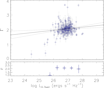
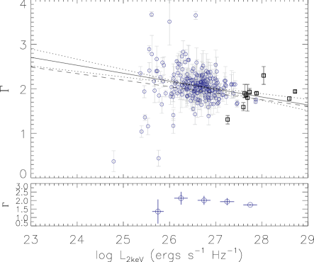
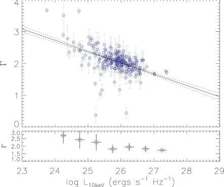
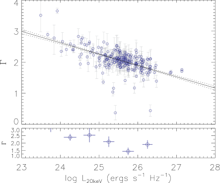
Figure 7: TOP: X-ray photon index ($\Gamma$) vs. monochromatic X-ray luminosity at rest-frame (a) 0.7 keV, (b) 2 keV, (c) 10 keV, and (d) 20 keV. In (b), the Green et al. (2008) correlation is plotted for comparison as a dashed line, and the quasars from Dai et al. (2004) are over-plotted as open black squares. Only RQ, non-BAL quasars are plotted (blue circles) The weighted least squares regression line is calculated using RQ, non-BAL quasars, and is plotted as a solid line, with errors shown as dotted lines. BOTTOM: The weighted mean $\Gamma$ values are given for bins of width $\Delta$log L_2-10keV = 0.5. Error lines mark the 1$\sigma$ dispersions in both axes. Blue lines represent RQ+non-BAL quasars, while green lines represent RL+non-BAL quasars.

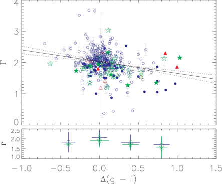
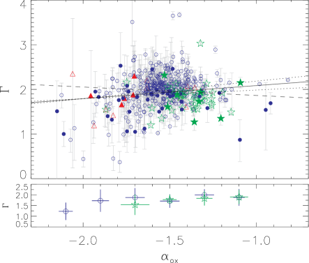
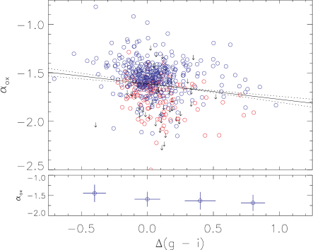
Figure 9: TOP: (a) $\Gamma$ vs. $\alpha_{ox}$, with the $\Gamma-\alpha_{ox}$ correlation found by Green et al. (2008) plotted for comparison as a dashed line. (b) $\Gamma$ vs. $\Delta$($g-i$), the relative ($g-i$) color, for sources with z $<$ 2.3. Symbols for (a) and (b) are as in Figure 7, though the correlations are determined only for RQ, non-BAL and non-absorbed quasars. Weighted least square regressions are plotted as solid lines, with 3$\sigma$ errors shown as dotted lines. (c) $\alpha_{ox}$ vs. relative ($g-i$) color for sources with z $<$ 2.3. Symbols for (c) are as in Figure 5. We plot the OLS regression as a solid line, with 1$\sigma$ errors shown as dotted lines. BOTTOM: The weighted mean $\Gamma$ values are given for bin widths as follows: (a) $\Delta\alpha_{ox}$ = 0.2, (b) $\Delta$[$\Delta$($g-i$)] = 0.3, and (c) $\Delta$[$\Delta$($g-i$)] = 0.4. Error lines mark the 1$\sigma$ dispersions in both axes. Blue lines represent RQ+non-BAL quasars, while green lines represent RL+non-BAL quasars. Figure (c) does not include BAL or RL quasars.

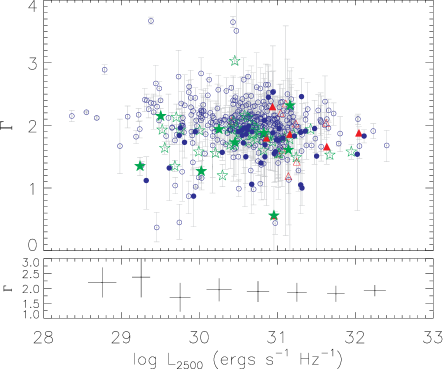
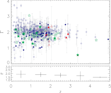
Figure 11: X-ray photon index ($\Gamma$) vs. (a) optical 2500 Å monochromatic luminosity and (b) redshift. Blue circles represent RQ, non-BAL quasars, green stars represent RL quasars, and red triangles represent BAL quasars. Filled symbols are given for those sources that prefer an absorbed power-law with an F-test probability P $>$ 0.95. The bottom plots show the weighted mean $\Gamma$ values for bins of width (a) $\Delta$log L₂₅₀₀ = 0.5 and (b) $\Delta$z = 1.

Nevertheless, the amount of absorption in this sample is only a lower-limit for two reasons. First, undetected absorption may still exist, particularly in low S/N sources. For example, in the correlation plots (e.g. Figures 7,9 and 11), three sources can be seen with $\Gamma\sim$ 0.5. These sources do not formally prefer either absorption model, but their X-ray spectra are cut off at soft energies, suggesting absorption as the likely cause of flat spectra. Second, we cannot test for absorption in sources with S/N $<$ 6, and it is possible that these low S/N sources have a higher percentage of absorption.

For the 55 sources that prefer absorption , we calculate the weighted mean of the intrinsic column density: N_H = 1.5$\pm$0.3 x 10²¹ cm^-2. The absorbed population consists of 6 broad absorption line objects (BAL), 7 radio-loud (RL), and 42 radio-quiet (RQ), non-BAL objects.

Table 3 summarizes the weighted means of $\alpha_{ox}$, $\Gamma$ and N_H for the three sub-sets of quasar populations: RQ+non-BAL, RL+non-BAL, and BAL. (There are four quasars that are both RL and BALs.) Because of the small numbers of absorbed spectra in the sub-populations, comparing the respective N_H distributions is not meaningful, but $\alpha_{ox}$ and $\Gamma$, Kolmogorov-Smirnov (K-S) tests show that the RQ distribution is significantly different from the RL distribution, with probabilities P_KS $<$ 0.5% that the two samples are drawn from the same parent distribution (Fig. 6). RL quasars are known to be brighter in the X-rays for a given 2500 Å luminosity (e.g. Zamorani et al., 1981). However, while RL quasars are also known to have flatter X-ray slopes than RQ quasars (Wilkes & Elvis, 1987; Williams et al., 1992; Reeves et al., 1997; Reeves & Turner, 2000; Page et al., 2005; Piconcelli et al., 2005), the average $\Gamma$ value for RL quasars in the SDSS/XMM sample ($<\Gamma>$ = 1.85 $\pm$ 0.04) is steeper than that found in previous samples ($<\Gamma>$ $\sim$ 1.5-1.75). Figure 6$b$ shows that RL quasars do follow the same Gaussian distribution as RQ quasars for $\Gamma<$ 1.9, but for $\Gamma>$ 1.9, the RL distribution falls off rapidly. Only 7 of 49 RL quasars (14%) have $\Gamma>$ 2, compared to 48% of RQ quasars.

The $\Gamma$ distribution is not significantly different for BAL vs. non-BAL quasars (P_KS = 75%) once the X-ray spectra are corrected for intrinsic absorption. However, the $\alpha_{ox}$ distribution of BAL quasars, which includes 37 sources with S/N $<$ 6 that cannot be corrected for absorption, remains significantly different (P_KS = 0.2%) from non-BAL quasars. Previous studies have noted the difference in X-ray brightness for BAL quasars (e.g. Green & Mathur, 1996).

4.1 Correlations with the X-ray Spectral Slope

The large number of X-ray spectra in the SDSS/XMM Quasar Survey allows us to test for correlations with the X-ray photon index ($\Gamma$). Since we use only sources detected with a high enough S/N to fit a power-law, we do not use survival statistics and instead use the Kendall’s rank correlation coefficient to test for correlations. We use only those sources that do not prefer either absorption model, and we also require that the SPL model result in a reasonably good fit ($\chi^{2}_{\nu}<1.2$). In addition, we restrict the selection to those sources with S/N $>$ 10 in order to reduce the effect of undetected absorption in lower S/N spectra.

When correlations are significant, we plot a Weighted Least Squares (WLS) regression line to take into account the measurement errors in $\Gamma$, which are much larger than the errors in the independent variable. RQ quasars show two correlations of $\Gamma$ with luminosity and optical color with probabilities less than 0.5% that they are due to chance: (1) $\Gamma$ vs. log L_2keV (P_K = 2.4e-5) and (2) $\Gamma$ vs. $\Delta$($g-i$) (P_K = 7.5e-4), where P_K is the Kendall rank two-sided significance level for each correlation. RQ quasars also show a marginal correlation between $\Gamma$ and $\alpha_{ox}$ (P_K = 1.6%). The $\Gamma$ - L_2keV, $\Gamma$ - $\Delta$($g-i$) and $\Gamma$ - $\alpha_{ox}$ relations are not significant (P${}_{K}>$ 10%) for RL quasars (green stars in Figures 7, 9 and 11). We now discuss each of these correlations in turn.

4.1.1 X-ray Slope vs. X-ray Luminosity

An anti-correlation exists between the X-ray slope ($\Gamma$) and the 2 keV luminosity (log L_2keV), hereafter $l_{2keV}$, such that X-ray slopes harden as X-ray luminosity increases (Fig. 7$a$). The WLS regression line (for RQ, non-BAL quasars) is:

$$\Gamma=(6.39\pm 1.3)+(-0.16\pm 0.05)l_{2keV}$$ (1)

To investigate the possibility of a pivot point in the X-ray spectrum, we next examined 7 additional correlations between the X-ray slope ($\Gamma$) and the monochromatic X-ray luminosities at 0.7, 1, 1.5, 4, 7, 10 and 20 keV. The monochromatic fluxes are obtained for sources preferring the SPL model by normalizing the fit at each energy in turn. The results of these correlations are summarized in Figures 7$a-d$ and in Table 4. The strength of the correlation increases with energy as the slope steepens, so the strongest, steepest correlation is between $\Gamma$ and $l_{20keV}$ (Fig. 7$d$). Correlation strength decreases at lower energies, bottoming out at 1 keV, where the slope is consistent with zero. At 0.7 keV, the slope flips to a positive correlation and the strength of the correlation increases again. The flip in the correlation slope indicates a pivot in the X-ray spectrum near 1 keV (Fig. 8$a$).

For the correlations above, we have used $\Gamma$ to extrapolate the rest-frame monochromatic luminosities for sources with redshifts out of range of the observed spectrum. To check that this extrapolation does not affect the correlations, we perform the fits again, this time excluding any sources where the rest-frame luminosity is not in the observed range. The results are shown in Table 5, and plotted in Fig. 8$b$. The errors are larger, due to the smaller sample sizes and the narrower range of luminosities observed, but the spectrum still pivots between 1 and 1.5 keV. At the lowest energies, the slopes become much steeper, possibly due to the influence of a soft excess component on the power-law fit.

The $\Gamma$ determined from the SPL model is used to determine the monochromatic flux, so it is important to check that the model assumptions do not induce the observed anti-correlation. To do this, we re-fit the sources, this time with a power-law fixed to the sample mean ($\Gamma$ = 1.91) and intrinsic absorption fixed to zero. We then obtain the monochromatic flux at 2 keV and compare the F_2keV obtained via a fixed power-law to the F_2keV obtained via the best-fit power-law. We find that changing the model assumptions changes the log flux values by 1.4%, which is not enough to explain the observed correlation at 2 keV.

Even with the selection restricted to sources with S/N $>$ 10, there is still the possibility of undetected absorption. For example, Figures 7 show two sources with $\Gamma$ $\sim$ 0.5 and another four radio-quiet sources with $\Gamma$ $\sim$ 1-1.5. The X-ray spectra of these sources show curvature in the soft X-rays that, while not significant enough for the sources to prefer an absorption model, nevertheless suggests that intrinsic absorption is the likely cause of flat X-ray slopes. Therefore, we test for correlations again, this time using sources with S/N $>$ 20 in order to minimize the chance of undetected absorption. The significance of the correlation increases, with the probability of a chance correlation falling below P_K = 1e-7. However, with many low-luminosity sources eliminated, the correlation is biased to a steeper slope. Having shown that the correlations do not rely on undetected absorption, we continue to use the correlations for sources with S/N $>$ 10 for further analysis.

The slope of the $\Gamma-l_{2keV}$ anti-correlation is equivalent within errors to the slope found in Green et al. (2008). They also find a correlation between $\Gamma$ and the 2 keV luminosity based on 156 RQ and RL quasars fit with a power-law plus intrinsic absorption, plus 979 quasars with lower S/N that were fit with a single power-law and zero intrinsic absorption. A similar anti-correlation between $\Gamma$ and 2-10 keV luminosity was found in Page et al. (2005) for 16 RL quasars. While the Page et al. (2005) correlation was not found to be significant for RQ quasars, there were only 7 RQ quasars in their sample. However, a previous study by Dai et al. (2004) found the opposite correlation between $\Gamma$ and $l_{2-10keV}$ at 98.6% significance for a sample of 10 quasars observed with Chandra and XMM. The $\Gamma$ and extrapolated $l_{2keV}$ values for the Dai et al. (2004) quasars are plotted in Fig. 7$a$ as open, black squares, where they are consistent with the trend observed in SDSS-XMM quasars. The SDSS/XMM-Newton Quasar Survey increases the sample size of previous studies by factors of 3 - 30, and covers $\sim 3$ decades of X-ray luminosity.

To explain the observed correlations between $\Gamma$ and X-ray luminosity, we must answer two questions:

1. Why does the X-ray slope change with luminosity?

2. Why does the slope change such that the pivot point is near 1 keV?

We address two possible answers to the first question. First, an increased hard component at higher X-ray luminosities may explain the trends observed here. The hard component may be due to nonthermal emission associated with a jet (e.g. Zamorani et al., 1981; Wilkes & Elvis, 1987) or due to a reflection component (Krolik, 1999). RL quasars do not show a significant correlation between $\Gamma$ and L_X except for marginal correlations at high energies (7 and 10 keV), but this may be because a jet already dominates the X-ray emission. The spectrum of the hard component may flatten the X-ray spectrum by covering up the steeper power-law due to inverse Compton scattering, while simultaneously increasing the 2-10 keV luminosity.

Alternatively, quasars with low X-ray luminosities may have steeper slopes due to a component linked to high accretion rates. As discussed in $\S$1.1, previous studies have found a strong correlation between $\Gamma$ and the Eddington ratio (L_bol/L_Edd), where steeper sources are associated with higher accretion rates. Therefore, sources with high accretion rates (and steep X-ray spectra) must be associated with low X-ray luminosity in order to produce the $\Gamma$-L_X correlations. However, it is not clear if high accretion rates and steep X-ray spectra tend to coincide with low X-ray luminosity. Studies of X-ray binary (XRB) accretion states have shown that high accretion states tend to be associated with steep X-ray spectra and high X-ray flux compared to the low accretion state (Remillard & McClintock, 2006). However, the distinction is not clear in every source - even ”high” accretion states can be associated with both low and high X-ray flux. Narrow-line Seyfert 1 (NLS1) galaxies are an extreme example of high accretion rate objects (Boroson, 2002), but while they typically have steep X-ray slopes, their X-ray flux can range from X-ray bright to weak (e.g., $\alpha_{ox}$ = 0.7-2.2 Leighly, 1999). The $\Gamma$-L_bol/L_Edd relation for the SDSS/XMM-Newton Quasar Survey will be discussed further in (Risaliti et al. 2009, in prep.).

Inverse Compton scattering of UV photons from an accretion disk in a hot corona could explain why the X-ray spectrum pivots at low X-ray energies. In the corona model, the X-ray spectrum will change shape if the temperature (T_e) and/or optical depth ($\tau$) of the corona vary (Rybicki & Lightman, 1979), since the output spectrum flattens as the $y$ parameter increases. The $y$ parameter is the average fractional energy gained by a photon; for a thermal, non-relativistic electron distribution,

$$y=\frac{4kT_{e}}{m_{e}c^{2}}max(\tau,\tau^{2})$$ (2)

For example, if the disk emission brightens, increasing the soft photon supply, the corona will increase radiative cooling to maintain temperature balance, producing a steeper X-ray spectrum. For a T $\sim$ 10⁸-10⁹ K corona, opacity is not necessarily dependent on luminosity, so opacity variations can result in a pivot in the 2-10 keV band without a large accompanying change in luminosity (Haardt et al., 1997).

Because of the relation between the physical parameters and the output spectrum, it is possible to calculate T${}_{e}\tau$, though the degeneracy is not breakable without knowing the cut-off of the high-energy spectrum. From Krolik (p. 227-8, 1999),

$$\ T_{e}\tau\sim a~{}(l_{h}/l_{s})^{1/4}\sim a~{}\frac{-1.6}{\Gamma-1},$$

where $a$ is a coefficient dependent on geometry ($a$ = 0.06 for slabs) and $l_{h}/l_{s}$ is the compactness ratio, equivalent to the heating rate over the soft photon seed supply. Therefore, as $\Gamma$ changes from 2.3 at low luminosities to 1.8 at high luminosities, T${}_{e}\tau$ approximately doubles from 4.16 x 10⁸ to 7.13 x 10⁸ K.

Several studies have found evidence of pivot points in individual objects. The previous paragraph describes the model of Mrk766, a NLS1, which was found to pivot near $\sim$10 keV (Haardt et al., 1997). In Cygnus X-1, a black hole X-ray binary, Zdziarski et al. (2002) find a negative correlation between X-ray flux and $\Gamma$ for the 0.15-12 keV band; no correlation for the 20-100 keV band; and a positive correlation for flux greater than 100 keV, implying a pivot point near $\sim$50 keV. Zdziarski et al. (2002) model this spectrum as a variable supply of soft seed photons irradiating a thermal plasma, where optical depth is constant. An increase in seed flux results in a decrease in the corona temperature to satisfy energy balance, resulting in a steeper spectrum with a pivot somewhere below 100 keV. Two model-independent analyses of the spectral variability in Seyfert 1 galaxies also show evidence of pivot points. NGC 4051 was found to have a pivot near 50 keV using correlations between the 2-5 keV and 7-15 keV fluxes (Taylor et al., 2003), and NGC 5548, studied with an 8-day BeppoSAX observation (Nicastro et al., 2000), can be entirely explained by a pivot in the medium energy band ($\sim$6 keV). While these examples show that pivot points may exist in X-ray spectra, it is clear that further exploration must be done to provide a clear picture of the underlying physics.

4.1.2 X-ray slope vs. optical color and $\alpha_{ox}$ (for RQ quasars only)

X-ray slope ($\Gamma$) and optical color [$\Delta$($g-i$)] are correlated at 3.4$\sigma$, such that quasars with redder colors are more likely to have flat X-ray slopes (Fig. 9$a$). This is likely due to undetected absorption, which is discussed further below. We exclude sources with redshifts greater than 2.3 from the $\Gamma$ - $\Delta$($g-i$) correlation as Ly$\alpha$ absorption artificially reddens high-redshift quasars. The linear bisector is:

$$\Gamma=(2.04\pm 0.02)+(-0.45\pm 0.10)\Delta(g-i)$$ (3)

The $\Gamma$ - $\Delta$($g-i$) correlation is consistent with previous findings of a correlation between $\Gamma$ and the optical/UV spectral slope ($\alpha_{uv}$) (Kelly et al., 2007) because color correlates tightly with the optical slope (Richards et al., 2003) ($\Delta$($g-i$) $\propto$ 0.5 $\alpha_{uv}$). The slope of the correlation in this paper is in the same direction as, but steeper than in Kelly et al. (2007), who find a slope = -0.25 $\pm$0.07.

X-ray slope ($\Gamma$) anticorrelates with $\alpha_{ox}$ at marginal (2.4$\sigma$) significance, such that X-ray faint quasars are more likely to have flat X-ray slopes (Fig. 9$b$). The WLS regression line is:

$$\Gamma=(2.8\pm 0.2)+(0.6\pm 0.1)\alpha_{ox}$$ (4)

This anti-correlation between $\Gamma$ and $\alpha_{ox}$ contrasts with the slightly positive correlation found by Green et al. (2008) (overplotted as the almost horizontal dashed line in Fig. 8$b$). The Green et al. (2008) correlation may be affected by the inclusion of RL quasars, which lie at the X-ray bright end and typically have flatter X-ray slopes than RQ quasars.

Completing the triangle of relations, a correlation is found between $\alpha_{ox}$ and $\Delta$($g-i$) at 4.7$\sigma$ significance (Fig. 9$c$). Again, sources with redshifts greater than 2.3 are excluded in order to avoid contamination by the Ly$\alpha$ forest. Since the $\alpha_{ox}$-$\Delta$($g-i$) relation includes censored data, we use the EM method to give the best-fit line:

$$\alpha_{ox}=(-1.613\pm 0.009)+(-0.16\pm 0.04)\Delta(g-i)$$ (5)

The EM algorithm assumes that all of the error lies in the dependent variable, so the algorithm reduces to an OLS Y vs. X fit for uncensored data.

In an attempt to disentangle the relationships between $\Gamma$, $\Delta$($g-i$), and $\alpha_{ox}$, we perform the Kendall partial correlation test for sources with S/N $>$ 6 and z $<$ 2.3, but each correlation is significant at the $\sim$3$\sigma$ level even when the third variable is taken into account. The dispersions in all three relations are large, so the sources are binned along the x-axis to show the relationships more clearly. The binning shows that the relations are dominated by outliers: optically red and X-ray weak/flat sources.

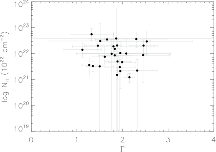
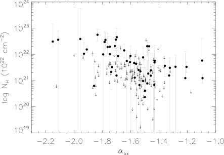
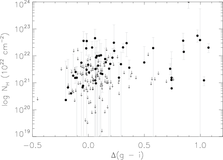
Figure 10: (a) Intrinsic absorption (N_H) vs. $\Gamma$. (b) N_H vs. $\alpha_{ox}$. (c) N_H vs. $\Delta$($g-i$). The solid circles in (a) and (b) represent sources preferring the APL model, while in (c) the solid circles represent sources preferring either absorption model (FPL or APL). The arrows represent sources with only a 90% upper-limit on N_H. N_H is given in log units of 10²² cm^-2.

Detected absorption cannot explain the observed correlations with $\Gamma$, since sources are only included if they do not prefer a model with intrinsic X-ray absorption. $\Gamma$ is not correlated with N_H (Fig. 10$a$) for sources that prefer the APL model, indicating that once the X-ray slope is corrected for absorption, no intrinsic correlation between X-ray slope and absorption remains. For the same sources, $\alpha_{ox}$ and N_H (Fig. 10$b$) correlate at the 3.3$\sigma$ level, which is surprising since the 2 keV flux should also be corrected for absorption. Since the detections trace the upper-limits, this correlation is likely not intrinsic, but is due to the survey flux limit. The optical color also depends on absorption (Fig. 10$c$) at the 2.6$\sigma$ level, as is expected, since X-ray absorbed sources are more likely to have redder colors due to dust-reddening.

Undetected absorption is a possible explanation for all three relations, causing red optical colors and X-ray weakness while flattening the X-ray spectral slope in low S/N spectra. A simple calculation shows that the amounts of absorption obtained from equations (3) and (4) are consistent with observed gas-to-dust ratios observed for quasars. First, we assume that both relations are driven entirely by the effects of absorption (i.e. ignoring any possible effects due to intrinsic properties, such as black hole mass and accretion rate). We also assume that an unabsorbed quasar has a typical X-ray slope, ($\Gamma$ = 1.9), zero absorption (N_H = 0 and E_B-V = 0), and typical blue optical colors ($\Delta$($g-i$) = 0). If the X-ray slope changes by a given amount, we can calculate the change in color by equation (3), which corresponds to a dust-reddening (Richards et al., 2003), which in turn leads to a change in optical luminosity. Since the X-ray slope also gives $\alpha_{ox}$ by equation (4), we can calculate the change in X-ray luminosity at 2 keV, which in turn gives the intrinsic X-ray absorption. So for an absorbed quasar with $\Gamma$ = 1.4, the dust-reddening is E(B-V) = 0.096 from equation (3), the gas column is N_H $\sim$ 6 x 10²² cm^-2 from equation (4), giving a gas-to-dust ratio $\sim$ 100 times the Galactic value. Quasars typically have gas-to-dust ratios in the range of 10-100 times the Galactic value (Maccacaro et al., 1981; Maiolino et al., 2001; Wilkes et al., 2002), so relations (3) and (4) are consistent with intrinsic absorption that remains undetected in the X-ray spectra.

Intrinsic absorption is less likely to remain undetected in spectra with high S/N. As a second test, we restrict the correlation tests to those sources with X-ray S/N $>$ 20. As a result, all three correlations disappear, which again supports undetected absorption as the cause of correlations that include low S/N sources.

4.1.3 X-ray slope vs. redshift and optical luminosity

Neither redshift nor 2500 Å luminosity correlate significantly with $\Gamma$ ($P_{S}>$ 10%, Figures 11), confirming previous studies with smaller samples (Page et al., 2004; Risaliti et al., 2005; Shemmer et al., 2005; Vignali et al., 2005; Kelly et al., 2007). Note however Bechtold et al. (2003), who find that X-ray slopes are flatter at lower redshifts for a sample of 17 radio-quiet, high-redshift (3.7 $<$ z $<$ 6.3) quasars observed with Chandra. The SDSS/XMM sample (473 sources with X-ray spectra) is at least an order of magnitude larger than these previous samples, though it does not have homogenous spectral coverage for redshifts above 2.5.

5 Conclusions and Future Work

We have cross-correlated the DR5 SDSS Quasar Catalog with the XMM-Newton archive, creating a sample of 792 quasars with a detection rate of 87%. Almost 500 quasars have X-ray spectra, the largest sample available for analysis of optical/X-ray spectral correlations. We find that the X-ray photon index $\Gamma$ correlates significantly with $l_{X}$, where X = 2, 4, 7, 10 and 20 keV. Optical color and $\alpha_{ox}$ also correlate with $\Gamma$, but these correlations are likely due to the effect undetected intrinsic absorption rather than intrinsic physical changes. The X-ray slope does not correlate significantly with redshift or optical luminosity. With a sample size at least an order of magnitude larger than previous studies, we confirm a highly significant correlation between $\alpha_{ox}$ and the monochromatic luminosity at 2500 Å, and we also confirm that $\alpha_{ox}$ does not correlate significantly with redshift or optical color.

Future studies of the sample will include: $\alpha_{ox}$, $\Gamma$ vs optical properties, and studies of sub-populations such as BALs and Type 2 quasars. Variability studies will also be pursued for 265 objects with multiple XMM observations. More complex spectral analysis on high X-ray S/N sources will include a thermal component for the soft excess, warm absorbers, and emission line detection.

6 Erratum: The Fifth Data Release Sloan Digital Sky Survey/XMM-NEWTON Quasar Survey (2009, ApJS, 183, 17); published Nov. 3, 2009

We have discovered an error in column 9 of Table 2 in the original paper. This column reports the fit flags, indicating which model a source prefers: a simple power-law (SPL, flag = 1), a fixed power-law plus intrinsic absorption (FPL, flag = 2), or an absorbed power-law (APL, flag = 3). The table of the original paper mistakenly reports all flag=3 sources as having flag=2, and all flag=2 sources as having flag=1, so that only 32 sources prefer an absorption model.

We have updated Table 2 to print out the correct fit flags for each source, resulting in 55 sources that prefer an absorption model. Since the fit flags determine which numbers are reported for the remaining columns of Table 2, these numbers are updated as well. The abstract and text of the original paper report the correct number of absorbed sources, so the conclusions are unaffected.

In addition, a minor rounding error was found in the SDSS names of some objects, and so we replace both Table 1 and 2 with corrected versions. Corrected machine-readable tables are available online from ApJS and will soon be available on the High Energy Astrophysics Science Archive Resource Center (HEASARC, http://heasarc.gsfc.nasa.gov).

Table 1: SDSS quasars with archival XMM-Newton observations

SDSS name	XMM ID	z	NH,gal	(S/N)X	Exp.	$\Theta$	Net	Background	RL	BAL
					time		counts	counts	flag	flag
SDSS J125930.97+282705.5	0204040101	1.094	0.92	18.0	221.0	13.4	469	103.	0	0
SDSS J130120.13+282137.2	0204040101	1.369	0.94	45.8	221.0	13.2	2780	449.	1	0
SDSS J114856.56+525425.2	0204260101	1.633	1.37	23.0	9.4	5.8	620	52.1	1	0
SDSS J215419.70-091753.6	0204310101	1.212	3.71	12.5	81.3	10.9	218	43.5	0	0
SDSS J164221.22+390333.4	0204340101	1.713	1.22	11.3	45.7	11.9	182	39.1	0	0
SDSS J021000.22-100354.2	0204340201	1.960	2.20	13.2	31.6	10.9	243	47.0	1	0
SDSS J021100.83-095138.4	0204340201	0.767	2.17	14.4	31.6	11.8	268	40.6	0	0
SDSS J123508.19+393020.0	0204400101	0.968	1.49	9.9	65.5	4.8	153	42.8	0	0
SDSS J123527.36+392824.0	0204400101	2.158	1.49	20.1	89.8	6.0	553	104.	0	0
SDSS J133812.97+391527.1	0204651101	0.439	0.86	18.7	23.1	8.0	416	38.4	0	0

Note. — Table 1 is presented in its entirety in the electronic edition of the Astrophysical Journal. A portion is shown here for guidance regarding its form and content. The upper limits are at the 1.6$\sigma$ level.

Table 2: X-ray Spectral Data of SDSS Quasars

SDSSname	f0.5-2	f2-10	f0.5-2	f2-10	L0.5-2	L2-10	$\alpha_{ox}$	Fit	$\Gamma$	NH	$\chi^{2}/\nu$
	(obs.)	(obs.)	(rest)	(rest)	(rest)	(rest)		flag
SDSS J125930.97+282705.5	0.94	5.20	0.41	2.46	0.27	1.61	-1.77	1	0.99${}_{-0.14}^{+0.13}$	$<$3.10	38.9/28
SDSS J130120.13+282137.2	12.4	20.5	9.01	17.0	10.3	19.3	-1.32	1	1.78${}_{-0.07}^{+0.07}$	$<$0.05	90.0/120
SDSS J114856.56+525425.2	26.3	59.9	14.0	39.5	24.5	69.4	-1.60	1	1.58${}_{-0.12}^{+0.12}$	$<$0.73	20.3/26
SDSS J215419.70-091753.6	1.51	2.38	0.93	2.10	0.79	1.77	-2.12	1	1.87${}_{-0.27}^{+0.29}$	$<$0.68	5.0/12
SDSS J164221.22+390333.4	3.09	6.23	1.76	4.39	3.48	8.68	-1.52	1	1.66${}_{-0.24}^{+0.25}$	$<$0.44	4.5/12
SDSS J021000.22-100354.2	5.63	12.7	2.35	8.04	6.49	22.1	-1.37	1	1.60${}_{-0.19}^{+0.19}$	$<$1.38	7.9/14
SDSS J021100.83-095138.4	5.72	5.04	5.72	5.73	1.56	1.56	-1.41	1	2.23${}_{-0.22}^{+0.24}$	$<$0.19	5.6/16
SDSS J123508.19+393020.0	1.68	1.45	1.74	1.69	0.84	0.82	-1.52	1	2.23${}_{-0.33}^{+0.38}$	$<$0.65	5.1/13
SDSS J123527.36+392824.0	2.57	3.40	1.57	3.13	5.49	10.9	-1.51	1	1.94${}_{-0.16}^{+0.17}$	$<$0.54	20.7/25
SDSS J133812.97+391527.1	9.13	38.0	6.69	28.2	0.47	1.98	-1.50	1	1.17${}_{-0.16}^{+0.17}$	$<$0.08	14.1/22

Note. — Table 2 is presented in its entirety in the electronic edition of the Astrophysical Journal. A portion is shown here for guidance regarding its form and content.Luminosities are computed using H₀ = 70 km s^-1 Mpc^-1, $\Omega_{M}$ = 0.3, and $\Omega_{\Lambda}$ = 0.7. The upper limits are at the 1.6$\sigma$ level.

Table 3: Weighted Averages of X-ray Spectral Quantities

	Ndet	$\alpha_{ox}$	Nspec	$\Gamma$	$\sigma_{\Gamma}$	$\sigma_{\Gamma,intr}$	NH
All	685	-1.60	473	1.90$\pm$0.02	0.40	0.37	0.15$\pm$0.03
RQ+non-BAL	589	-1.61	411	1.91$\pm$0.08	0.41	0.38	0.14$\pm$0.04
RL+non-BAL	62	-1.46	47	1.85$\pm$0.03	0.30	0.26	0.15$\pm$0.03
BAL	34	-1.78	15	1.96$\pm$0.05	0.37	0.34	2.3$\pm$0.6

Table 4: $\Gamma$ - L_X Correlations

E (keV)	PK	Z-level	slope	intercept	dispersion
0.7	0.0062	2.73	0.095$\pm$0.058	-0.500$\pm$1.564	0.36
1.0	0.1683	0.16	-0.015$\pm$0.054	2.462$\pm$1.449	0.37
1.5	0.0033	1.77	-0.106$\pm$0.051	4.903$\pm$1.363	0.37
2.0	0.0000	2.93	-0.162$\pm$0.048	6.386$\pm$1.286	0.37
4.0	0.0000	5.61	-0.265$\pm$0.041	9.042$\pm$1.082	0.35
7.0	0.0000	7.50	-0.316$\pm$0.035	10.28$\pm$0.917	0.33
10.0	0.0000	8.60	-0.335$\pm$0.032	10.73$\pm$0.818	0.31
20.0	0.0000	9.61	-0.365$\pm$0.027	11.38$\pm$0.690	0.29

Table 5: $\Gamma$ - L_X Correlations with redshift cut-offs

E (keV)	PK	sig	slope	intercept	dispersion
0.7	0.0112	2.54$\sigma$	0.583$\pm$0.285	-13.29$\pm$7.587	0.46
1.0	0.0386	1.43$\sigma$	0.196$\pm$0.129	3.077$\pm$3.447	0.44
1.5	0.0024	2.07$\sigma$	-0.120$\pm$0.058	5.270$\pm$1.363	0.38
2.0	0.0000	3.03$\sigma$	-0.162$\pm$0.053	6.800$\pm$1.417	0.38
4.0	0.0000	5.64$\sigma$	-0.178$\pm$0.044	9.596$\pm$1.176	0.35
7.0	0.0000	7.49$\sigma$	-0.337$\pm$0.038	10.84$\pm$0.986	0.33
10.0	0.0000	8.60$\sigma$	-0.355$\pm$0.034	11.25$\pm$0.874	0.31
20.0	0.0000	7.03$\sigma$	-0.293$\pm$0.129	9.560$\pm$3.342	0.22

Figure 2: Survey characteristics: (a) Exposure time histogram, where exposure times are summed over the up to three EPIC cameras. Exposure times do not include high-background intervals filtered out during data reduction. (b) S/N histogram, where 16 sources have X-ray S/N $>$ 100. (c) Fraction of detected sources vs. redshift, and (d) redshift histogram. For (c) and (d), the open, dotted-line histogram is for all SDSS-selected quasars, the open, solid-line histogram is for all detected sources, the hatched histogram is for sources with sources with X-ray S/N $>$ 6, and the double-hatched histogram is for sources with X-ray S/N $>$ 10.

Figure 3: $\chi^{2}_{\nu}$ histogram. The open histogram represents sources that prefer a power-law model. The solid histogram represents sources that prefer an absorbed power-law model. Five sources have $\chi^{2}_{\nu}$ $>$ 2 and are not included in the plot.

Figure 4: X-ray and optical sensitivity: (a) Optical 2500 Å luminosity vs. redshift and (b) X-ray 2-10 keV luminosity vs. redshift. Flux limits are plotted in both plots. For (a), $i$ band magnitude limits (dotted lines) were set during selection (Richards et al., 2002). For (b), the flux limit (log F_2-10keV = -14.0 ergs cm^-2 s^-1, dotted line) is for an observation of 20 ks (Watson et al., 2001). (c) The observed-frame F_2-10keV distribution.

Figure 6: (a) $\alpha_{ox}$ distribution for all sources. (b) $\Gamma$ distribution for sources with S/N $>$ 6. Open histograms represent RQ, non-BAL quasars and have been scaled down by factors of 3 and 4, respectively. Histograms with vertical hatching represent RL quasars, and histograms with diagonal hatching represent BAL quasars. The space above the upper-limit arrows indicates the number of RQ+non-BAL upper-limits in a given bar.

Figure 8: The slope of the $\Gamma$-L_X correlation vs. energy E with 1$\sigma$ errors on the slope for (a) all sources and (b) sources where the rest-frame energy lies in the observed range. The slopes of the $\Gamma$-L_X correlations are obtained for E = 0.7, 1, 1.5, 2, 4, 7, 10, and 20 keV, and are marked as solid circles. The Green et al. (2008) correlation slope is marked as an open circle at 2 keV. A dashed line marks zero.

References

- Adelman-McCarthy et al. (2007) Adelman-McCarthy et al. 2007, ApJS 172, 634
- Akylas et al. (2004) Akylas A., Georgakakis A. & Georgantopoulos I. 2004, MNRAS, 353, 1015
- Anderson & Margon (1987) Anderson S.F. & Margon B. 1987, ApJ, 314, 111
- Avni, Worrall & Margon (1995) Avni Y., Worrall D.M. & Margon W.A. 1995, ApJ, 454, 673
- Avni & Tananbaum (1982) Avni Y. & Tananbaum H. 1982, ApJ, 262, L17
- Bechtold et al. (2003) Bechtold J. et al. 2003, ApJ, 588, 119
- Bevington et al. (1992) Bevington, P. R. & Robinson, D. K. 1992, Data Reduction and Error Analysis for the Physical Sciences (2d ed; New York: McGraw-Hill)
- Boller et al. (1996) Boller T., Brandt W. N. & Fink H. 1996, A&A, 305, 53
- Boroson & Green (1992) Boroson, T. A., & Green, R. F. 1992, ApJS, 80, 109
- Boroson (2002) Boroson T.A. 2002, ApJ, 565, 78
- Braccesi et al. (1970) Braccesi, A., Formiggini, L., Gandolfi, E. 1970, A&A, 5, 264
- Brandt et al. (1997) Brandt W.N., Mathur S. & Elvis M. 1997, MNRAS, 285, L25
- Brandt & Boller (1998) Brandt, N., & Boller, T. 1998, Astron. Nachr., 319, 163
- Cash (1979) Cash W. 1979, ApJ, 228, 939
- Cordova et al. (1992) Cordova F.A., Kartje J.F., Thompson R.J., Mason K.O., Puchnarewicz E.M., Harnden F.R. 1992, ApJS, 81, 661
- Croom et al. (2001) Croom, S.M., Smith, R.J., Boyle, B.J., Shanks, T., Loaring, N.S., Miller, L. & Lewis, I.J. 2001, MNRAS, 322, L29
- Dai et al. (2004) Dai X., Chartas G., Eracleous M. & Garmire G.P. 2004, ApJ, 605, 45
- den Herder et al. (2001) den Herder, J. W., Brinkmann, A. C., Kahn, S. M., et al. 2001, A&A, 365, L7
- Dickey & Lockman (1990) Dickey J.M. & Lockman F.J. 1990, ARAA, 28, 215
- Elvis et al. (1994) Elvis M. et al. 1994, ApJ, 95, 1
- Giaconni et al. (1974) Giacconi R. & Gursky H. (ed.) X-ray Astronomy, 1974, Astrophysics and Space Science Library, 43, 304
- Gibson et al. (2009) Gibson R.R. et al. 2009, accepted to ApJ, astroph/0810.2747
- Green & Mathur (1996) Green P. & Mathur S. 1996, ApJ, 462, 637
- Green et al. (2001) Green P., Aldcroft T., Mathur S., Wilkes B. & Elvis M. 2001, ApJ, 558, 109
- Green et al. (2003) Green et al. 2003, AN, 324, 93
- Green et al. (2008) Green et al. 2008, submitted to ApJS
- Haardt & Maraschi (1991) Haardt F. & Maraschi L. 1991, ApJ, 380, L51
- Haardt et al. (1997) Haardt F., Maraschi L. & Ghisellini G. 1997, ApJ, 476, 620
- Hall et al. (2006) Hall P., Gallagher S., Richards G.T., Alexander D.M., Anderson S.F., Bauer F., Brandt W.N. & Schneider D.P. 2006, AJ, 132, 1977
- Hewett et al. (1995) Hewett P. C., Foltz C. B. & Chaffee F. H. 1995, AJ, 109, 1498
- Hopkins et al. (2004) Hopkins P. et al. 2004, AJ, 128, 1112
- Just et al. (2007) Just D.W., Brandt W.N. Shemmer O., Steffen A.T., Schneider D.P., Chartas G. & Garmire G.P. 2007, ApJ, 665, 1004
- Kalberla et al. (2005) Kalberla et al. 2005, A&A, 440, 775
- Kawaguchi et al. (2001) Kawaguchi T., Shimura T. & Mineshige S. 2001, ApJ, 546, 966
- Kellerman et al. (1989) Kellerman K., Sramek R., Schmidt M., Shaffer D. & Green R. 1989, AJ, 98, 4
- Kelly et al. (2007) Kelly B.C., Bechtold J., Siemiginowska A., Aldcroft T. & Sobolewska M. 2007, ApJ, 657, 116
- Kelly et al. (2008) Kelly B.C., Bechtold J., Trump J.R., Vestergaard M., Siemiginowska A. 2008, ApJS, 176, 355
- Kembhavi & Narlikar (1999) Khembavi A.K. & Narlikar J. V. 1999, Quasars and Active Galactic Nuclei: An Introduction (Cambridge, UK: Cambridge University Press)
- Komossa (2007) Komossa S. astroph/0710.3326K
- Kriss & Canizares (1985) Kriss G.A. & Canazares C.R. 1985, ApJ, 297, 177
- Krolik (1999) Krolik J.H. 1999, Active Galactic Nuclei: From the Central Black Hole to the Galactic Environment (Princeton: Princeton University Press), 198
- Laor et al. (1997) Laor A., Fiore F., Elvis M., Wilkes B.J. & McDowell J.C. 1997, ApJ, 477, 93
- Laor (2000) Laor A. 2000, NewAR, 44, 503
- Lavalley et al. (1992) Lavalley M., Isobe T. & Feigelson E. 1992, ASPC, 25, 245L
- Leighly (1999) Leighly K. M., 1999, ApJS, 125, 317
- Lumb et al. (2002) Lumb D.H., Warwick R.S., Page M., & De Luca A. 2002, A&A, 389, 93
- Maccacaro et al. (1981) Maccacaro T., Perola G. C., & Elvis M. 1981, ApJ, 246, L11
- Maiolino et al. (2001) Maiolino R., Marconi A., Salvati M., Risaliti G., Severgnini E.O., La Franca F. & Vanzi L. 2001, A&A, 365, 28
- Mainieri et al. (2007) Mainieri et al. 2007, ApJ, 172, 368
- Malkan & Sargent (1982) Malkan M. & Sargent W. 1982, ApJ, 254, 22
- Maraschi et al. (1991) Maraschi L., Chiappetti L., Falomo R., Garilli B., Malkan M., Tagliaferri G., Tanzi E.G. & Treves A. 1991, ApJ, 368, 138
- Markarian (1967) Markarian B.E. 1967, Astrofizika, 3, 55
- Markarian et al. (1981) Markaryan B. E., Lipovetskii V. A. & Stepanyan, Dzh A. 1981, Ap, 17, 321
- Mateos et al. (2005) Mateos et al. 2005, A&A, 433, 855
- Nicastro et al. (2000) Nicastro F. et al. 2000, ApJ, 536, 718
- Nousek & Shue (1989) Nousek J.A. & Shue D.R. 1989, ApJ, 342,1207
- Osmer & Smith (1980) Osmer, P.S. & Smith, M.G. 1980, ApJS, 42, 333
- Osmer (1981) Osmer, P.S. 1981, ApJ, 247, 762
- Page et al. (2003) Page K.L., Turner M.J.L., Reeves J.N., O’Brien P.T. & Sembay S. 2003, MNRAS, 338, 1004
- Page et al. (2004) Page K.L., Reeves J.N., O’Brien P.T., Turner M.J.L. & Worrall D.M. 2004, MNRAS, 353, 133
- Page et al. (2005) Page K.L., Reeves J.N., O’Brien P.T. & Turner M.J.L. 2005, MNRAS, 364, 195
- Pickering et al. (1994) Pickering T.E., Impey C.D. & Foltz C.B. 1994, AJ, 108, 5
- Piconcelli et al. (2005) Piconcelli E., Jimenez-Bailón E., Guainazzi M., Schartel N., Rodríguez-Pascual P.M. & Santos-Lleo M. 2005, A&A, 432, 15
- Pier et al. (2003) Pier J.R., Munn J.A., Hindsley R.B., Hennessy G.S., Kent S.M., Lupton R.H. & Izezic Z. 2003, AJ, 125, 1559
- Pierre et al. (2007) Pierre M. et al. 2007, MNRAS, 382, 279
- Reeves & Turner (2000) Reeves J. N., Turner M. J. L., 2000, MNRAS, 316, 234
- Reeves et al. (1997) Reeves J. N., Turner M. J. L., Ohashi T., Kii T., 1997, MNRAS, 292, 468
- Remillard & McClintock (2006) Remillard R.A. & McClintock J.E. 2006, ARAA, 44, 49
- Richards et al. (2002) Richards et al. 2002, AJ, 123, 2945
- Richards et al. (2003) Richards et al. 2003, AJ, 126, 1131
- Risaliti et al. (2003) Risaliti G., Elvis M., Gilli R. & Salvati M. 2003, ApJ, 587, L9
- Risaliti et al. (2005) Risaliti G. & Elvis M. 2005, ApJ, 629, L17
- Risaliti et al. (2009) Risaliti G., Young M. & Elvis M. 2008, in preparation
- Rybicki & Lightman (1979) Rybicki G.B. & Lightman A.P. 1979, Radiative Processes in Astrophysics (New York:John Wiley & Sons), 208-222
- Saez et al. (2008) Saez C. et al. 2008, astroph/08013599v1
- Schmidt & Green (1983) Schmidt M. & Green R.F. 1983, ApJ, 269, 352
- Schneider et al. (2007) Schneider D. P.et al. 2007, AJ, 134, 102
- Shakura & Sunyaev (1973) Shakura N.I. & Sunyaev R.A. 1973, A&A, 24, 337
- Shen et al. (2006) Shen S., White S.D.M.,Mo H.M., Voges W., Kauffmann G., Tremonti C., & Anderson S. F. 2006, MNRAS, 369, 1639
- Shen et al. (2008a) Shen Y., Strauss M.A., Hall P.B., Schneider D.P., York D.G., & Bahcall N.A. 2008, ApJ, 677, 858
- Shen et al. (2008b) Shen Y., Greene J., Strauss M., Richards G. & Schneider D. 2008, ApJ, 680, 169
- Shemmer et al. (2005) Shemmer et al. 2005, ApJ, 630, 729
- Shemmer et al. (2006) Shemmer O., Brandt W.N., Netzer H., Maiolino R. & Kaspi S. 2006, ApJ, 646, L29
- Shemmer et al. (2008) Shemmer O., Brandt W.N., Netzer H., Maiolino R. & Kaspi S. 2008, astroph/0804.0803
- Shields et al. (1978) Shields G.A. 1978, Nature, 272, 706
- Spergel et al. (2003) Spergel D.N. et al. 2003, ApJS, 148, 175
- Steffen et al. (2006) Steffen A., Strateva I., Brandt W., Alexander D., Koekemoer A., Lehmer B., Schneider D. & Vignali C. 2006, AJ, 131, 2826
- Strateva et al. (2005) Strateva I.V., Brandt W.N., Schneider D.P., Vanden Berk D.G. & Vignali C. 2005, ApJ, 130, 387
- Strueder et al. (2001) Strueder L. et al. 2001, A&A, 365, L18
- Tananbaum et al. (1979) Tananbaum H. et al. 1979, ApJ, 234, L9
- Tananbaum et al. (1986) Tananbaum H., Avni Y., Green R.F., Schmidt M. & Zamorani G. 1986, ApJ, 305, 57
- Tang et al. (2007) Tang S.M., Zhang S.N. & Hopkins P. 2007, MNRAS, 377, 1113
- Taylor et al. (2003) Taylor R.D., Uttley P. & McHardy I.M. 2003, MNRAS,342, L31
- Trump et al. (2007) Trump J.R. et al. 2007, ApJS, 165, 1
- Turner et al. (2001) Turner M. et al. 2001, A&A, 365, L27
- Vanden Berk et al. (2005) Vanden Berk D.E. et al. 2005, AJ, 129, 2047
- Vignali et al. (2003) Vignali C., Brandt W.N. & Schneider D.P. 2002, AJ, 125, 443
- Vignali et al. (2005) Vignali C., Brandt W.N., Schneider D.P. & Kaspi S. 2005, AJ, 129, 2519
- Ward et al. (1987) Ward M.J., Elvis M., Fabbiano G., Carleton N.P., Willner S.P. & Lawrence A. 1987, ApJ, 315, 74
- Warren et al. (1991) Warren S.J., Hewett P.C., Irwin M.J., & Osmer P.S. 1991, ApJS, 76, 1
- Watson et al. (2001) Watson M. et al. 2001, A&A, 365, L51
- Watson et al. (2008) Watson M.G. 2008, Astron. Nachr., 329, 131
- Weisskopf (1991) Weisskopf M. astroph/9912097v1
- Weymann et al. (1991) Weymann R.J., Morris S.L., Foltz C.B., & Hewett P.C. 1991, ApJ, 373, 23
- Wilkes & Elvis (1987) Wilkes B.J. & Elvis M. 1987, ApJ, 323, 243
- Wilkes et al. (2002) Wilkes B.J., Schmidt G.D., Cutri R.M., Ghosh, H., Hines D.C., Nelson B. & Smith P.S. 2002, ApJ, 564, L65
- Williams et al. (1992) Williams O. R. et al., 1992, ApJ, 389, 157
- White et al. (1997) White R., Becker R., Helfand D. & Gregg M. 1997, ApJ, 475, 479
- Wilkes et al. (1994) Wilkes B.J., Tananbaum H., Worrall D.M., Avni Y., Oey M.S. & Flanagan J. 1994, ApJS, 92, 52
- York et al. (2000) York et al. 2000, AJ, 120, 1579
- Young et al. (2008) Young M., Elvis M. & Risaliti G. 2008, ApJ, 688, 1
- Young et al. (2009b) Young M., Elvis M. & Risaliti G. 2009, in preparation
- Yuan et al. (1998) Yuan W., Siebert J. & Brinkmann, W. 1998, AA, 334, 498
- Zamorani et al. (1981) Zamorani G. et al. 1981, ApJ, 245, 357
- Zdziarski et al. (2000) Zdziarski A.A., Poutanen J. & Johnson W.N. 2000, ApJ, 542, 703
- Zdziarski et al. (2002) Zdziarski A.A., Poutanen J., Paciesas W.S. & Wen L. 2002, ApJ, 578, 357
- Zhou et al. (2006) Zhou H., Wang T., Yuan W., Lu H., Dong X., Wang J. & Lu Y. 2006, ApJS, 166, 128