Near-Infrared Light Curves of the Brown Dwarf Eclipsing Binary 2MASS J05352184–0546085: Can Spots Explain the Temperature Reversal?
Abstract
We present near-infrared JHKS light curves for the double-lined eclipsing binary system 2MASS J05352184-0546085 (catalog ), in which both components have been shown to be brown dwarfs with an age of Myr. We analyze these light curves together with the previously published -band light curve and radial velocities to provide refined measurements of the system’s physical parameters. The component masses and radii are here determined with an accuracy of % and %, respectively. In addition, we confirm the previous surprising finding that the primary brown dwarf has a cooler effective temperature than its lower-mass companion. Next, we perform a detailed study of the residual variations in the out-of-eclipse phases of the light curves to ascertain the properties of any inhomogeneities (e.g. spots) on the surfaces of the brown dwarfs. Our analysis reveals two low-amplitude ( mag) periodic signals, one attributable to the rotation of the primary with a period of d and the other to the rotation of the secondary with a period of d. Both periods are consistent with the measured and radii. Finally, we explore the effects on the derived physical parameters of the system when spots are included in the modeling of the light curves. The observed low-amplitude rotational modulations are well fit by cool spots covering a small fraction (%) of the brown dwarfs’ surfaces. Such small spots negligibly affect the physical properties of the brown dwarfs, and thus by themselves cannot explain the primary’s unexpectedly low surface temperature. To mimic the observed K suppression of the primary’s temperature, our model requires that the primary possess a very large spot coverage fraction of %. These spots must in addition be symmetrically distributed on the primary’s surface so as to not produce photometric variations larger than observed. Altogether, a spot configuration in which the primary is heavily spotted while the secondary is lightly spotted—consistent with the idea that the primary’s magnetic field is much stronger than the secondary’s—can explain the apparent temperature reversal and can bring the temperatures of the brown dwarfs into agreement with the predictions of theoretical models.
1 Introduction
Empirical measurements of the masses, radii, temperatures, and luminosities of pre–main-sequence (PMS) objects are valuable for the understanding of star formation. They delimit the Initial Mass Function, defining the outcome of star formation and giving the energy scale for the formation process. They represent the observational tie to the theoretical evolution models that describe the chronology of stellar evolution, setting the timescales for circumstellar disk evolution and planet formation. In order for these models to accurately describe the physics of PMS evolution, they must be tested against observed properties of young stars and brown dwarfs.
For PMS stars with masses lower than 2 M☉, there are currently only a few tens of objects published with these fundamental parameters determined with a precision better than 10% (e.g., Mathieu et al., 2007). Double-lined eclipsing binary systems allow for a distance independent, direct measurement of the masses, radii and, when absolute photometry is available, effective temperatures of the components. Among the techniques for obtaining dynamical masses, the spectro-photometric modeling of eclipsing binary systems is the only that provides radii for both components, but more importantly it also renders the most accurate mass measurements. If light and radial velocity curves for both components are available, then the absolute dimensions of the system may be obtained (e.g. Andersen et al., 1983).
The discovery of the system 2MASS J05352184–0546085 (hereafter 2M053505), the first eclipsing binary system comprised of two brown dwarfs, was presented by Stassun et al. (2006), hereafter Paper I. With a reported period of = 9.779621 0.000042 d, 2M053505 was found as part of a photometric survey searching for variability in the Orion Nebula Cluster. Through the simultaneous radial velocity and -band light curve analysis of this fully detached system, they obtained masses of = 0.054 0.005 M☉ and = 0.034 0.003 M☉ for the primary and secondary components, respectively, with corresponding radii of = 0.669 0.018 R☉ and = 0.511 0.026 R☉. They found a surprising reversal of surface brightnesses in which the less massive component radiates more per unit surface area (i.e. has a higher effective temperature) than the more massive one, contrary to what is expected for coeval brown dwarfs (Baraffe et al., 1998).
A follow-up analysis of 2M053505 was presented by Stassun et al. (2007) (hereafter Paper II) in which it was suggested that the apparent temperature reversal in 2M053505 could be the result of preferentially strong magnetic activity on the primary brown dwarf. This hypothesis was shown by Chabrier et al. (2007) to be theoretically plausible, and was then reinforced empirically when Reiners et al. (2007) found that the primary brown dwarf rotates faster and exhibits stronger H emission than the secondary. One manifestation of enhanced activity on the primary brown dwarf should be the presence of large, cool surface spots (Chabrier et al., 2007). If present, such spots should produce photometric variations that are periodically modulated by the rotation of the brown dwarf. Indeed, the presence of low-amplitude variations in the -band light curve of 2M053505 was noted in Paper II, however an analysis of such variation was deferred to the present paper.
This paper broadens the previous analyses of 2M053505 with the addition of near-infrared (JHKS) light curves, and investigates the intrinsic variability of the light curves in more detail. The near-infrared observations and their reduction are described in Sec. 2 and analyzed in Sec. 3. A periodicity analysis of the out-of-eclipse phases of the light curves in Sec. 3.1 yields the rotation periods of the two components of the binary to be d and d, consistent with the measured by Reiners et al. (2007) and the previously measured radii. The modeling of the JHKS light curves together with the previously published light curve and radial velocity data is described in Sec. 3.2, from which we determine refined measurements of the system’s physical parameters. The apparent temperature reversal found in the previous studies is confirmed yet again.
Sec. 4 incorporates surface spots into the light curve modeling. In particular, we assess the properties (areal coverage and temperature) of the spots that are required to both reproduce the observed low-amplitude variations and permit the surrounding photospheric temperatures of the two brown dwarfs to be in agreement with theoretical expectation for young brown dwarfs. We find that a small cool spot (% areal coverage and % cooler than the surrounding photosphere) on each of the brown dwarfs can reproduce the observed low-amplitude variations. Then, by introducing additional spots that uniformly cover % of the primary’s surface, we are able to simultaneously reproduce the observed surface brightness ratio of the two brown dwarfs (i.e. the apparent temperature reversal) while bringing the underlying temperature of the primary into agreement with the predictions of theoretical models. We discuss our findings in Sec. 5 and summarize our conclusions in Sec. 6.
2 Near-Infrared Light Curves
This paper focuses primarily on extending the published spectro-photometric analyses (Paper I, Paper II) of 2M053505 with the addition of the near-infrared photometric light curves in the (1.2 ), (1.6 ) and (2.2 ) passbands. The inclusion of more light curves in the modeling allows further constraint of the system’s parameters, in particular the temperatures and radii of the components. The multi-band analysis also probes the nature of the low-amplitude variability.
2.1 Near-Infrared Photometric Observations
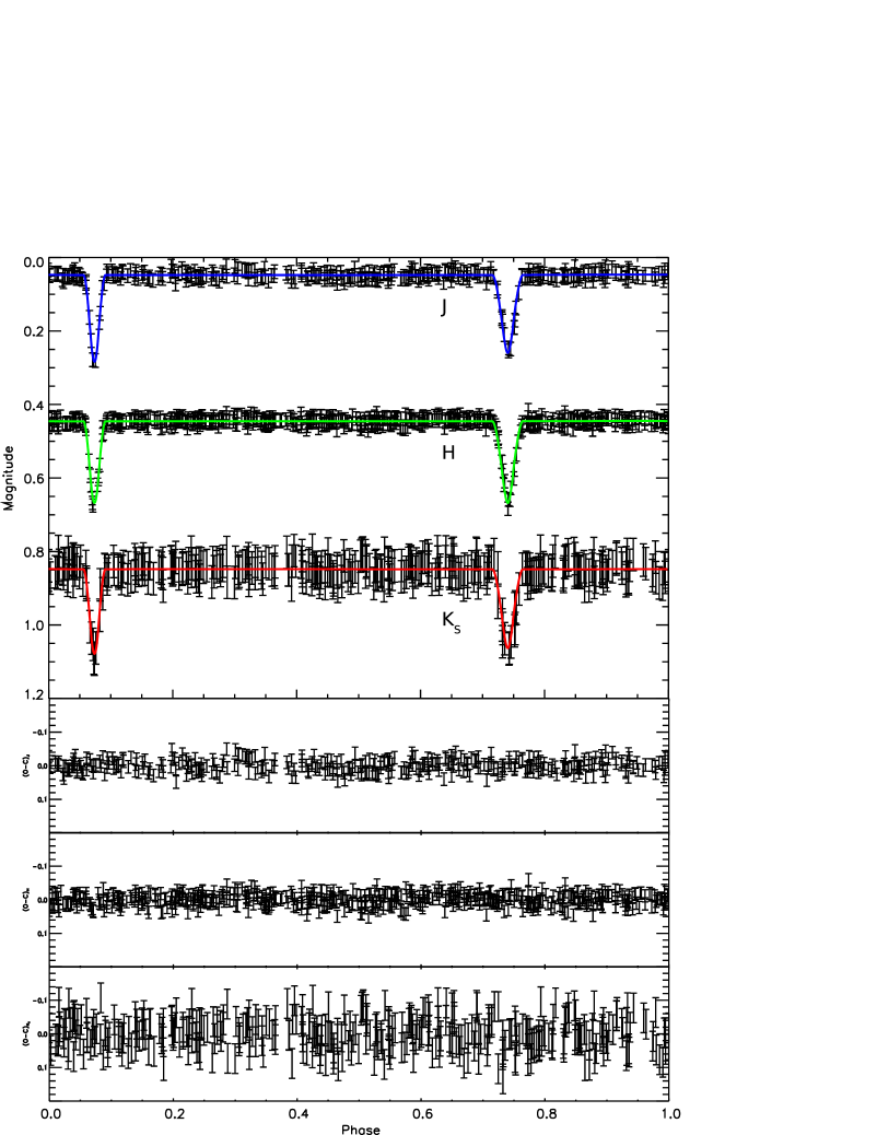
The observations of 2M053505 presented in this paper were taken in the 2MASS near-infrared bands JHKS from October 2003 to April 2006 at Cerro Tololo Inter-American Observatory in Chile. They were observed with the SMARTS 1.3-m telescope using the ANDICAM instrument which allows for simultaneous optical and infrared imaging (the optical measurements have been reported in Paper I and Paper II). The observations in the near-infrared were made in sets of 7 dither positions providing a total of 362 measurements in , 567 in and 385 in spread over five observing seasons. The integration times were typically of 490 seconds for the JHKS passbands. Table 1 describes the observing campaigns in full detail, while Tables 2–4 provide the individual measurements in the JHKS bands. The mean near-infrared magnitudes of 2M053505 are , , and (Skrutskie et al., 2006).
2.2 Data Reduction
The data were reduced differently depending on the dome flat acquisition. For observations made between October 2003 and March 2004, those comprising the data set I and affecting more than 50 percent of the light curve, the dome flats were obtained without information of the mirror’s position. A composite dome flat was created by subtracting a median combination of 10 images taken with the dome lights on minus the median combination of 10 images taken with the lights off in order to reduce the infrared contribution in the final images of sources such as the telescope, optical components and the sky. The procedure to then reduce data set I consisted of the following steps: a sky image is formed from the median combination of the 7 dithers; it was then normalized to the background of each individual image and subtracted from each separately; every image was then divided by the normalized flat; the dithers were aligned; the images were cropped, and they were combined by doing a pixel-by-pixel average.
For images taken from October 2004 onward, dome flats were provided individually for each of the 7 dither positions, proving essentially helpful in removing the interference pattern of sky emission lines characteristic to each of the mirror positions as well as the other infrared contributions. Each of the seven furnished dome flats follow the same combination as did the dome flats described in the previous paragraph. The individual dome flats for each of the mirror’s dithers allowed for the creation of separate flats for each mirror position. Sky flats were created from the median combination of 10 images with slightly different star fields for each distinct dither position, so that the stars present in the field averaged out and provided a flat image. This was possible since the observed field is not a very crowded one. For each of the remaining observing seasons, new sky flats were created in order to correct for any changes in the dithering and for any physical changes in the instrument. The reduction process is slightly different than for the first data set: the dark was first subtracted from the raw image; followed by the corresponding normalized sky flat, which depended on the mirror position at which the images were taken. The image was then divided by the corresponding normalized dome flat. Once this was done, the calibration resembles that of data set I: the dithered images were shifted and cropped in order to be median combined as to obtain the final image.
Differential aperture photometry was done using the IRAF package APPHOT. The comparison star was chosen because it appears in all of the reduced observations of 2M053505 and because it is non-variable in the -band observations. The phased JHKS light curves are presented in Fig. 1.
We are not able to directly measure the absolute photometric precision of the JHKS light curves because they depend on the assumption that the comparison star is non-variable, thus we do not report uncertainties on the individual differential photometric measurements in Tables 2-4. However, the standard deviation of the out-of-eclipse portions of the light curves gives a measure of the photometric scatter in each of the bands. While the light curves present a similar scatter, , the interference pattern of the sky emission lines is more significant in the band making the scatter larger, . As we show below, this photometric scatter includes low-amplitude intrinsic variations due to the rotation of 2M053505’s components.
3 Light Curve Analysis
The JHKS light curves described in the previous section are analyzed for periodicities apart from those due to the eclipsing nature of the binary (§3.1). Then they are modeled in conjunction with the available radial velocities and light curve in order to obtain the system’s physical parameters (§3.2). The thorough treatment of surface spots is introduced to the light curve solution in Sec. 4.
3.1 Rotation periods
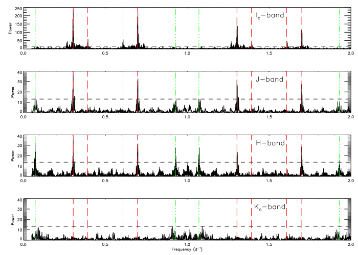
The light curves, both in the and the JHKS bands, present several periodicities. The most obvious period corresponds to that of the eclipses which recur on the orbital period, d (Stassun et al., 2007). In addition, the light curves in the observed bandpasses present a low-amplitude variability, with a peak-to-peak amplitude of 0.02–0.04 magnitudes, noticeable in the out-of-eclipse phases. We speculate that this type of periodic signal is due to the rotation of one or both components, resulting from spots on their surfaces rotating in and out of view (e.g., Bouvier et al., 1993; Stassun et al., 1999). Another possible explanation for the low-amplitude variations is intrinsic pulsation of one or both of the components. However, young brown dwarfs are expected to pulsate with periods of only a few hours (Palla and Baraffe, 2005) whereas we find periods of d and d (see below). Thus in what follows, for consistency we refer to these periods as and .
The light-curve data in the and JHKS bands corresponding to the out-of-eclipse phases were searched for periods between 0.1 and 20 d using the Lomb-Scargle periodogram (Scargle, 1982), well suited for unevenly sampled data. The resulting periodograms (Fig. 2) show the power spectra in frequency units of d-1 and present multiple strong peaks. These represent a combination of one or more true independent frequencies together with aliases due to the finite data sampling (Wall and Jenkins, 2003). The windowing of the data acquisition is of more relevance in the JHKS bands because a more significant aliasing is produced by including only data taken through the SMARTS queue observing which has a strong one-day sampling frequency.
The amplitudes of the periodograms are normalized according to the formulation of Horne and Baliunas (1986) by the total variance of the data, yielding the appropriate statistical behavior which allows for the calculation of the false-alarm probability (FAP). The FAP presents the statistical significance of the periodogram by describing the probability that a peak of such height would occur from pure noise. To calculate FAPs for the most significant peaks in the periodogram, a Monte Carlo bootstrapping method (e.g., Stassun et al., 1999) was applied; it randomizes the differential magnitudes, keeping the Julian Dates fixed in order to preserve the statistical characteristics of the data. One thousand random combinations of the out-of-eclipse magnitudes were done with this procedure to obtain the FAP in each band. The resulting 0.1% FAP level is indicated in the periodograms by the dashed line in Fig. 2. Except for the periodogram, multiple peaks are found well above the 0.1% FAP level and are therefore highly significant. The measurements are much noisier than in the bands (Sec. 2), so the lack of significant periodicity in that light curve is not surprising and we do not consider the light curve further in our periodicity analysis.
To distinguish the independent periods from their aliases, a sinusoid was fitted to each light curve and subtracted from the data in order to filter out the periodicity corresponding to the strongest peak in the periodograms. This peak in the bands is that which corresponds to the 3.293 0.001 d period previously identified in Paper II, at a frequency of 0.30 d-1. This period is not found in the light curve owing to a larger scatter of the data in that bandpass (§2.2). As expected, the subtraction of the 3.293-d periodic signal removed the strongest peak and also its aliases. The residual light curves were then reanalyzed to identify any additional periods.
This process revealed another independent frequency at 0.07 d-1 which corresponds to a period of 14.05 0.05 d. This 14.05-d period also manifests itself as a three-peaked structure centered at 1 d-1 in the bands. The two exterior peaks of this structure have frequencies of 0.93 and 1.07 d-1, corresponding to the beat frequencies between the 14.05-day period and a 1-day period. The 1-day period is most likely due to the sampling of the observations, since the bands were observed roughly once per night. The light curve does not show strong beats against a 1-day period because this band includes high-cadence data from many observing runs which disrupt the 1-day sampling period. The subsequent filtering of the 14.05-day period, as above, also removes its aliases and beats from the periodograms.
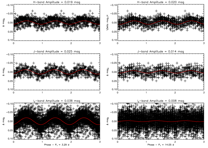
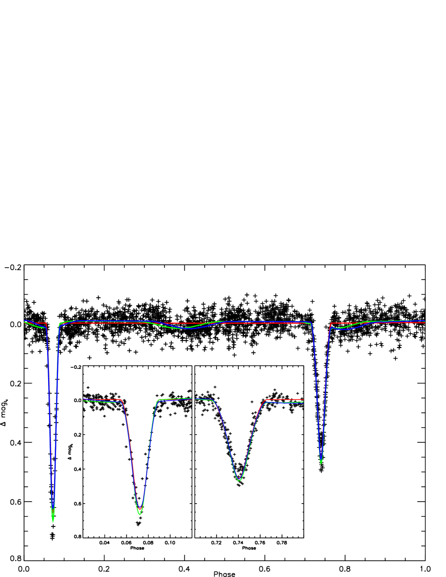
Fig. 3 shows the out-of-eclipse light curves of 2M053505 phased on these two periods, together with best-fit sinusoids to guide the eye and to quantify the amplitudes of the variability as a function of wavelength. Regardless of the order of the filtering, these two independent periods were always obtained via this analysis. No other significant periods are found. We furthermore confirmed that these periods were not present in the light curves of the comparison star used for the differential photometry (§2.2).
The uncertainty of the periods is given with a confidence interval of one sigma in the vicinity of the period peaks via the post mortem analysis described by Schwarzenberg-Czerny (1991). This method consists of determining the width of the periodogram’s peak at the mean noise power level. The 3.293-d period has 1- uncertainties of 0.001-d, 0.003-d and 0.002-d for the -, - and -band respectively; while for the 14.05-d period the 1- levels are 0.1-d for the -band and 0.05-d for the -band.
Reiners et al. (2007) reported measurements of 2M053505 to be km s-1 for the primary and km s-1 (upper limit) for the secondary, i.e., the primary rotates at least twice as fast as the secondary. Moreover, these values, together with the radii from Paper II and , correspond to rotation periods of d and d for the primary and secondary components, respectively. These are consistent with the periods of d and d that we have identified photometrically.
Table 5 summarizes the appearances of these two periods as a function of observing season and passband. The 3.29-d period is found consistently in nearly every season of observations in all three of the filters. We fit a sinusoid with a 3.29-d period separately to the data from each of the observing seasons and found that while the amplitude of the variability remained similar for each, the phase varied from season to season. Evidently, the 3.29-d period is caused by long-lived features that drift in longitude. The 14.05-d period is manifested less strongly in the data. While it is found in the light curves in most (but not all) seasons, it is detected in only two seasons of the -band data.
Interestingly, while the 3.29-d period manifests an increasing amplitude of variability toward shorter wavelengths (Fig. 3, left panels), as is expected for spots (either hot or cool; e.g. Bouvier et al., 1993), the amplitude of the 14.05-d periodicity declines toward shorter wavelengths. Maiti (2007) found a similar behavior in the optical variability of the field L dwarf 2MASSW J0036+1821, and suggested that the photometric variability in that object is therefore likely caused not by magnetic spots but rather by dust clouds formed near the surface (e.g. Zapatero Osorio et al., 2005). Perhaps the feature on the 2M053505 secondary that is responsible for the observed 14.05-d period is of similar origin. Indeed, this would be consistent with the findings of Reiners et al. (2007) that the 2M053505 secondary has a much weaker magnetic field compared to the primary, and thus may be less likely to produce strong magnetic spots.
In §4 below, we include spots in our modeling of the 2M053505 light curves in order to demonstrate the effects that spots may have on the properties of the magnetically active primary. The true physical nature of the inhomogeneity on the magnetically inactive secondary does not affect that analysis. For our purposes we emphasize that the 14.05-d period is consistent with the secondary’s measured and radius, and thus we can confidently ascribe that period to the rotation of the secondary.
3.2 Orbital and Physical Parameters of 2M053505
Light-curve solutions encompassing the multi-epoch, multi-band photometric data and radial-velocity measurements were calculated using the software PHOEBE (Prša and Zwitter, 2005) built on top of the 2007 version of the Wilson-Devinney algorithm (WD; Wilson and Devinney 1971). A square root limb-darkening law was adopted, its coefficients linearly interpolated by PHOEBE from the Van Hamme (1993) tables with each iteration. Emergent passband intensities are computed based on the passband transmission functions.
The simultaneous fit of the radial velocities and the JHKS light curves was done using the published results from Paper II as initial parameters for the modeling. The first column of Table 6 lists these starting values. The solution was then iterated. Since we do not have reliable errors on the individual JHKS measurements (see §2.2), the data points were assigned equal weight and then the overall weight of each light curves was set to the inverse-square of the r.m.s. of the residuals relative to the fit from the previous iteration. The primary’s temperature is taken to be K, where the uncertainty is dominated by the systematic uncertainty of the spectral-type– scale (Paper II). We emphasize that the uncertainty on the individual component temperatures does not represent the high accuracy with which the quantities directly involved in the light curve fitting are determined, namely the ratio of the temperatures. In addition to setting to a fixed value, the orbital period was also kept constant. The synchronicity parameters are obtained from the rotation periods (§3.1) such that and . The free parameters to be obtained from the modeling were: the inclination angle , the semi-major axis , the orbital eccentricity , the argument of the periastron , the systemic radial velocity , the mass ratio and the secondary’s surface temperature , through the determination of the temperature ratio . Because the primary’s radius is small compared to the semi-major axis (), reflection effects are assumed to be negligible (reflection effects generally only become important for %; e.g. Wilson, 1990).
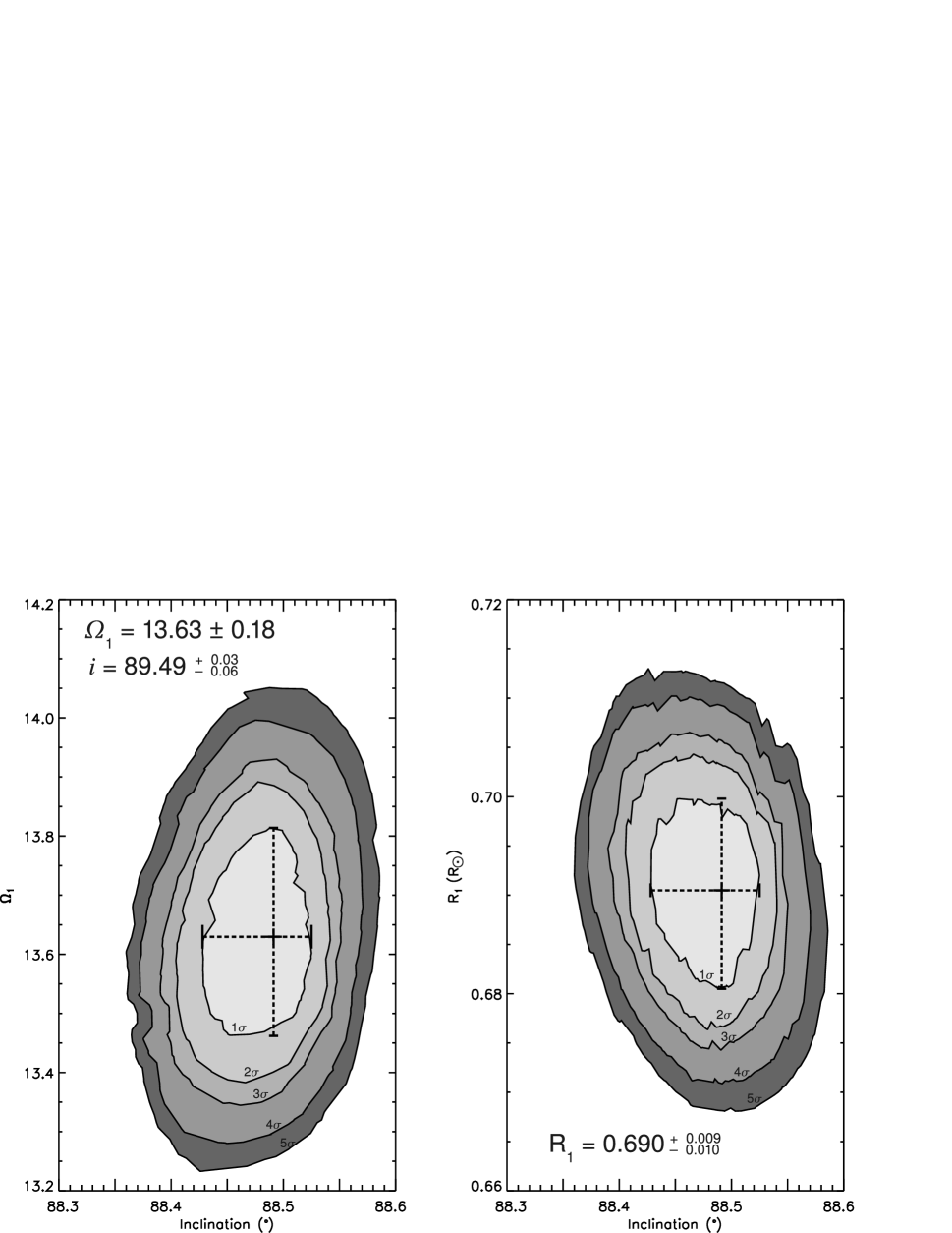
A direct output of the Wilson-Devinney algorithm that underlies PHOEBE is the formal statistical errors associated with each of the fit parameters, as well as a correlation matrix that provides insight into the often complex interdependencies of the parameters. In order to explore these parameter correlations and solution degeneracies more carefully, and to thus determine more robust parameter uncertainties, we performed a thorough Monte Carlo sampling of the parameter hyperspace using the PHOEBE code’s scripting capability. An examination of the parameter correlation matrix revealed that there are two particularly strong parameter degeneracies in our dataset: (1) between the inclination, , and the surface potentials, ; and (2) between the temperature ratio, , and the radius ratio, .
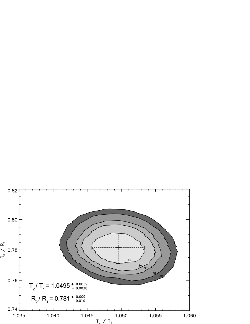
Fig. 4 shows the resulting joint confidence interval for and given by the variation of with these two parameters around the solution’s minimum. The shaded contours correspond to confidence intervals following a distribution with two degrees of freedom, with the first contour at the 1- confidence level and each subsequent level corresponding to an increment of 1 . The – cross section was sampled by randomly selecting a value for between 87∘ and 90∘, and one for between 12.0 and 14.5, rendering a more complete coverage of the parameter hyperspace. We marginalized over the remaining system parameters, notably the strongly correlated . This analysis yields uncertainties around the best-fit values of: degrees and , the latter corresponding to a primary radius of . The secondary’s best-fit radius and its uncertainties follow directly through the ratio of the radii (discussed in the next paragraph).
The – plane, shown in Fig. 5, is of particular interest because of the apparent temperature reversal that 2M053505 presents. This parameter cross section was explored keeping the of the primary fixed at 2715 K while varying the of the secondary between 2700 and 2925 K. The primary radius was varied randomly between 0.635 and 0.758 R☉, while minimizing for the secondary radius. The resulting uncertainties about the best-fit values are: and . Note that these errors determined from our Monte Carlo sampling procedure are larger than the formal statistical errors by 50%.
Finally, we separately performed a fit of the radial velocity data alone for the orbital parameters that most directly determine the masses, namely: , , and in order to more conservatively estimate the uncertainties in these parameters.These orbital parameters should not depend on the light curves, however we found that purely statistical correlations between these parameters and other system parameters tended to drive down the formal errors in the masses to unrealistically small values. We include , , and the time of periastron in the fit, but for these parameters we deferred error estimates to the simultaneous fit to the radial velocity and light curve data. Therefore we adopted the uncertainties in , , and from the radial velocity fit, the uncertainties in , , , and from the Monte Carlo sampling, and the uncertainties of other parameters from the simultaneous fit to the radial velocity and light curve data. We then propagated these uncertainties into the final errors of the parameters that depend on these quantities, such as the masses and radii.
The final parameters for 2M053505 resulting from our joint analysis of the radial velocities and JHKS light curves, and with uncertainties determined as described above, are summarized in the last column of Table 6. The results are in agreement with those previously published, although the uncertainties in many parameters have now improved compared to those reported in Paper II. For example, the uncertainties in the component masses has decreased from 10% to 6.5%, and the radii from % to 1.5%. This improvement arises primarily because of the improved determination of and through the addition of the JHKS light curves, thus improving the determination of the time of periastron passage.
As in the previous analyses of 2M053505 (Paper I, Paper II), we find again a reversal of effective temperatures from what would be expected from the observed mass ratio (i.e. the higher mass primary is cooler than the secondary) at high statistical significance. This surprising result is now confirmed on the basis of a full analysis including radial velocities and four light curves (JHKS) together.
4 Surface Spots
In §3.1 we found clear evidence of two separate low-amplitude variations in the light curves of 2M053505 with periods of 3.29 d and 14.05 d. PMS objects are typically found to be photometrically variable (e.g., Bouvier et al., 1993; Carpenter et al., 2001), and this variability is in almost all cases attributable to the presence of magnetic “spots” (akin to sunspots), to accretion from a circumstellar disk, or both. However 2M053505 has been shown to not possess circumstellar or circumbinary material and thus is not currently accreting (Mohanty et al., 2009). Pulsations have been suggested in a few brown dwarfs, but are expected to have characteristic periods of only a few hours (Palla and Baraffe, 2005).
In this section we explore the effects of surface spots on the light curves for the purpose of explaining the periodic variations found in §3.1, and to assess whether such spots might be able to explain the surprising reversal of effective temperatures in the system (§3.2).
We begin by determining the properties of spots on the primary required to reproduce the low-amplitude, periodic variability observed in the light curves. The primary’s variability amplitudes were measured by fitting a sum of two sinusoids to the out-of-eclipse data in each of the bands, one sinusoid corresponding to the rotation period of the primary at 3.293 d and another for the secondary at 14.05 d (Fig. 3). The amplitudes of the 3.29-d signal were then scaled up by the components’ relative luminosities, since the observed amplitudes are diluted by the light from the secondary.
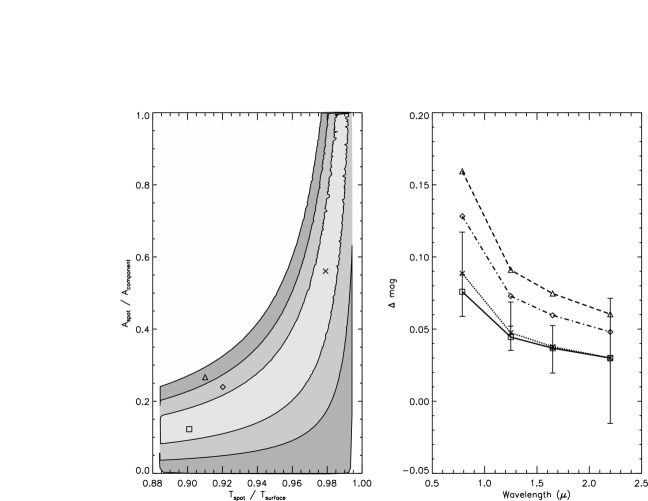
These amplitudes were fit using an analytic model based on a two-component blackbody as described by Bouvier et al. (1993). The free parameters are the spot temperature relative to the photosphere and the spot areal coverage. The areal coverage parameter is an “effective” area, i.e., it is really a measure of the ratio in spot coverage between the least and most spotted faces of the surface and is thus a measure of the degree of spot asymmetry. The results of this first-order analysis of the spot parameters are shown in Fig. 6. A family of solutions is found, such that a change in the spot temperature factor may be counterbalanced by a change in the areal coverage. As one example, the observed light-curve variations can be fit with a spot that is % cooler than the photosphere and that has an effective areal coverage of %. For the purposes of our modeling, and for simplicity, we placed a small cool spot with this temperature and area at the equator of the primary and allowed PHOEBE to adjust the spot’s longitude to match the phasing of the observed variations (Fig. 3). We emphasize that the spot parameters are degenerate and we do not claim that the adopted parameters are accurate in an absolute sense. Rather, they should be taken as representative of the asymmetric component of the primary’s spot distribution that causes the observed low-amplitude variability modulated on the primary’s 3.29-d rotation period (Fig. 3).
We ran a new light curve solution with PHOEBE, this time including the small spot on the primary as above, in order to check the influence of the spot specifically on the derived temperature ratio. The best-fit system parameters are changed insignificantly. The temperature ratio in particular is changed from the value in Table 6 by less than . This is not surprising given the small areal coverage and temperature contrast of the spot and considering that in Paper II we obtained a nearly identical temperature ratio with a purely spotless model. The inclusion of a small spot on the primary as required to fit the observed low-amplitude variability is by itself not sufficient to explain the observed temperature reversal in the system.
Therefore we next added a large cool spot at the pole of the primary. Assuming that the rotational and orbital axes of the system are parallel, and since , the effective areal coverage of a polar spot will not change with rotational phase as seen by the observer. Thus this polar spot represents the symmetric component of the primary’s spot distribution that, if it covers a sufficiently large area, may cause an overall suppression of the primary’s effective temperature without producing additional variations with rotational phase111In fact, even a polar spot will cause a small variation during eclipse, however this effect is % in the JHKS bands for the adopted spot parameters, and is thus below the threshold of detectability given our photometric precision of %.. The evolutionary models of Baraffe et al. (1998) predict an effective temperature of 2880 K for a brown dwarf with the mass of the 2M053505 primary at an age of 1 Myr, so we set the photospheric temperature of the primary to this value and re-fit the light curves with PHOEBE, this time including both a small equatorial spot as before together with a large polar spot as described above, both with temperatures 10% cooler than the photosphere. The areal coverages of the two spots were left as free parameters, and attained best-fit values of 8% and 65%, respectively.
Finally, we added a small equatorial spot on the secondary, again with a temperature 10% cooler than the photosphere, representing the surface inhomogeneity that produces the observed variations modulated on the secondary’s 14.05-d rotation period (Fig. 3). Using PHOEBE we performed a final simultaneous fit for the sizes of the spots on both the primary and secondary. The final best-fit spot areal coverage factors for the smal spot on the primary, the small spot on the secondary, and the large spot on the primary were 7%, 3%, and 65%, respectively.
In reality, the observed variability of the magnetically inactive secondary is not likely to be caused by a magnetic spot, but perhaps more likely by dust in its atmosphere (§3.1). Our light-curve modeling code does not currently incorporate a physical treatment of such dust features, and thus we use the spot modeling capability as a surrogate. In addition, we found that there is a near-total degeneracy between the sizes of the small spots on the primary and secondary if their temperatures are left as free parameters. That is, in the same way that the temperature and size of an individual spot are degenerate (see Fig. 6), the sizes of the two spots relative to one another are degenerate unless their temperatures are fixed. Thus we have taken the simplifying approach of fixing the spot temperatures to be 10% cooler than the surrounding photosphere on both the primary and secondary. The spot sizes are then constrained by the observed variability amplitudes (Fig. 3). Similarly, we have chosen not to include a large polar spot on the secondary as we have on the primary. The spot areas that we quote above are the formal best-fit values, however we caution that the properties we have determined for the inhomogeneity on the secondary should be taken as qualitative. More important for our analysis here, the properties of the spots on the magnetically active primary are minimally affected by the presence of the low-amplitude variability from the secondary, regardless of its true nature.
Finally, we have not included a polar spot on the secondary, although from the standpoint of the light curve modeling alone it is possible to achieve equivalent goodness-of-fit with polar spots on both components if their relative areal coverages are adjusted so as to preserve the adopted photospheric temperature ratio (see Fig. 7). We have taken the simplifying approach of including a polar spot on the primary only because (1) the evidence suggests that the primary is the more magnetically active of the two components (Reiners et al., 2007), (2) the secondary’s temperature is already in good agreement with the predictions of theoretical models (Paper II) and thus does not need to be suppressed by a large spot, and (3) as discussed above, the secondary’s variability amplitudes do not indicate that it possesses magnetic spots.
Fig. 8 presents a comparison of the spotted and unspotted light curve models for the band, the band in which the spot effects are most pronounced. The synthetic light curves shown have been calculated over a single orbital period. In view of the fact that the components do not rotate synchronously with one another or with the orbital period, the effects of the spots on the light curves (such as the dip in the model at a phase of 0.4) will shift in orbital phase from one orbit to the next, and thus these variations are averaged out in the observed light curve which is phased over many orbital periods. We furthermore verified that the effects of the spots on the radial velocities are negligible and thus do not affect any of the system’s physical parameters that are determined kinematically (e.g. the masses).
The primary conclusion to be drawn from the above is that the light curves of 2M053505 can be well modeled by having the primary component’s photospheric temperature at the theoretically expected value if % of its surface is covered with cool spots in a roughly symmetric distribution. The small spot in our model represents the % asymmetry in the spot distribution that produces the observed low-amplitude periodic variations.
5 Discussion
In order to simultaneously explain the observed low-amplitude variations and the anomalously low effective temperature of the primary (more massive) component in 2M053505, we have produced a model that includes a simple spot configuration of a small equatorial spot together with a very large polar spot. The former represents the asymmetric component of the spot distribution that produces the low-amplitude variations modulated on the primary’s rotation period, while the latter represents the symmetric component of the spot distribution that causes an overall suppression of the effective temperature below its theoretically predicted value. In this model, the unspotted regions of the primary’s surface have the theoretically predicted value of 2880 K (Baraffe et al., 1998).
The true distribution of spots on the primary’s surface is probably more complex. For example, a more realistic spot configuration might be one that resembles Jupiter’s bands. In that case, a symmetric equatorial band with a temperature 10% cooler than the photosphere and extending above and below the equator would reproduce similarly the effect of the polar spot. The same result could be obtained by a leopard-print pattern as that described by Linnell (1991) with an equivalent areal coverage and equal spot temperature factor as the polar spot we modeled. Either of these might describe more accurately a physical configuration of spots for the primary. Without direct Doppler imaging of 2M053505, it is not possible to more accurately pinpoint the true spot properties.
We emphasize that there is nothing in our treatment of spots that prefers the primary’s effective temperature to be 2880 K as dictated by the evolutionary models. We could have chosen any other effective temperature for the photosphere surrounding the spots and achieved an equally good fit of the light curves by adjusting the spot temperature and/or areal coverage to compensate. Thus our adoption of a primary effective temperature of 2880 K in the light curve solution of Fig. 8 should not be interpreted as a verification of the theoretical models. In addition, it should be noted that in our model the overall surface brightnesses of the components (integrating over both spotted and unspotted surface regions) are unchanged, such that the primary’s overall effective temperature is still lower than that of the secondary. This is an unavoidable consequence of the observed eclipse depths, which ultimately require the secondary to be effectively hotter than the primary. The luminosities of the brown dwarfs thus also remain the same regardless of the chosen effective temperature and corresponding spot configuration, because the overall surface brightnesses and radii are unaltered by our spot treatment.
Moreover, our modeling of spots treats only the radiative behavior of the surfaces of the brown dwarfs, not their underlying structure. Consequently our modeling does not serve as a detailed test of any structural or evolutionary effects caused by the surface magnetism that is likely responsible for the spots that we have modeled. For example, Chabrier et al. (2007) have proposed that the temperature reversal in 2M053505 could be explained by a magnetically active primary with a spot covering fraction of 50% together with surface convection that has been magnetically suppressed to a very low (as opposed to the usual 1–2; e.g. Stassun et al., 2004). They also suggest that suppressed convection may explain why the measured radius of the primary is % larger than predicted by their theoretical mass-radius relationship. Their exploratory treatment assumes “black” (i.e. 0 K) spots, whereas our modeled spots have a more physically realistic temperature 10% cooler than the photosphere, so the total spot-covering fraction of % that we find for the primary (large polar spot plus small equatorial spot) may in fact be consistent with the % coverage adopted by Chabrier et al. (2007). In addition, we have empirically determined the radii of 2M053505 with an accuracy of %, however our light curve modeling cannot confirm whether the radii have been altered in some way by the presence of spots or by magnetically suppressed convection.
6 Summary
As the first known eclipsing binary where both components are brown dwarfs, 2M053505 is a paramount example against which theoretical brown dwarf formation and evolutionary models and other low-mass objects will be compared. Stassun et al. (2006) and Stassun et al. (2007) established the young and low-mass nature of the binary, and moreover identified a surprising reversal of temperatures in which the primary (more massive) brown dwarf is cooler than the secondary. Here, we reanalyze the previously published radial velocities and -band light curve together with newly obtained JHKS light curves. We confirm the surprising temperature reversal. In addition, our analysis improves the measurement of the system’s parameters and permits a detailed modeling of magnetic spots on the brown dwarfs that may be altering their surface properties.
The masses of the components priorly reported to have uncertainties of 10% (Paper II) have been here determined with an accuracy of 6.5%, and the radii with an accuracy of 1.5%. In addition, through a detailed analysis of the variability observed in the light curves out of eclipse, the rotation periods of both brown dwarfs are measured to be d and d. Thus the brown dwarfs rotate non-synchronously relative to the orbital motion and relative to one another, perhaps due to the youth of the system ( Myr; Stassun et al., 2006, 2007). These rotation periods are in agreement with those expected from the radii and the spectroscopically measured .
Reiners et al. (2007) have suggested that the rapid rotation of the primary brown dwarf, together with its strong emission, implies that it is strongly magnetically active. In addition, Chabrier et al. (2007) have proposed that a strong magnetic field on the primary could produce cool spots covering a large fraction of its surface, thereby suppressing its effective temperature and thus explaining why its temperature is lower than expected and apparently lower than the secondary’s.
In this paper we have demonstrated that a detailed spectro-photometric modeling of 2M053505 including the treatment of spots is consistent with these ideas and in particular is able to resolve the apparent reversal of the temperature ratio. In order to reconcile the observed effective temperatures with those predicted by theoretical models, the primary brown dwarf must be heavily spotted. This ‘spottedness’ must be more or less symmetric to agree with the low-amplitude variability observed in the light curves, and it must have large effective areal coverage. Thus we modeled a two-spot configuration on the primary’s surface: a large polar spot with an areal coverage of 65% to account for the lower-than-expected surface brightness, and an equatorial spot covering 10% of the surface for the purpose of introducing the asymmetry responsible for the observed low-amplitude photometric variability modulated on the rotation period. With this configuration, we are able to successfully reproduce the observed light curves with the primary having an effective temperature at the theoretically predicted value. Other geometries for the spot configuration—such as an equatorial band akin to those on Jupiter—would achieve the same effect.
To be clear, from the standpoint of the light-curve modeling alone there is no need for a large spot-covering fraction on either brown dwarf. A small areal coverage of 10% is sufficient to model the low-amplitude variations that we observe in the light curves. Our aim here has been to demonstrate as proof of concept that the spots on the primary are capable of explaining its suppressed effective temperature in a manner that is consistent both with recent empirical findings of enhanced activity on the primary (Reiners et al., 2007) and recent theoretical results on the effects of such activity on the physical properties of young brown dwarfs (Chabrier et al., 2007).
References
- Andersen et al. (1983) Andersen, J., J. V. Clausen, B. Nordstroem, and B. Reipurth, 1983, A&A 121, 271.
- Baraffe et al. (1998) Baraffe, I., G. Chabrier, F. Allard, and P. H. Hauschildt, 1998, A&A 337, 403.
- Bouvier et al. (1993) Bouvier, J., S. Cabrit, M. Fernandez, E. L. Martin, and J. M. Matthews, 1993, A&A 272, 176.
- Carpenter et al. (2001) Carpenter, J. M., L. A. Hillenbrand, and M. F. Skrutskie, 2001, AJ 121, 3160.
- Chabrier et al. (2007) Chabrier, G., J. Gallardo, and I. Baraffe, 2007, A&A 472, L17.
- D’Antona and Mazzitelli (1997) D’Antona, F., and I. Mazzitelli, 1997, Memorie della Societa Astronomica Italiana 68, 807.
- Horne and Baliunas (1986) Horne, J. H., and S. L. Baliunas, 1986, ApJ 302, 757.
- Linnell (1991) Linnell, A. P., 1991, ApJ 383, 330.
- Maiti (2007) Maiti, M., 2007, AJ 133, 1633.
- Mathieu et al. (2007) Mathieu, R. D., I. Baraffe, M. Simon, K. G. Stassun, and R. White, 2007, Protostars and Planets V , 411.
- Mohanty et al. (2009) Mohanty, S., K. G. Stassun, and R. D. Mathieu, 2009, ApJ 697, 713.
- Palla and Baraffe (2005) Palla, F., and I. Baraffe, 2005, A&A 432, L57.
- Prša and Zwitter (2005) Prša, A., and T. Zwitter, 2005, ApJ 628, 426.
- Reiners et al. (2007) Reiners, A., A. Seifahrt, K. G. Stassun, C. Melo, and R. D. Mathieu, 2007, ApJ 671, L149.
- Scargle (1982) Scargle, J. D., 1982, ApJ 263, 835.
- Schwarzenberg-Czerny (1991) Schwarzenberg-Czerny, A., 1991, MNRAS 253, 198.
- Skrutskie et al. (2006) Skrutskie, M. F., R. M. Cutri, R. Stiening, M. D. Weinberg, S. Schneider, J. M. Carpenter, C. Beichman, R. Capps, T. Chester, J. Elias, J. Huchra, J. Liebert, et al., 2006, AJ 131, 1163.
- Stassun et al. (1999) Stassun, K. G., R. D. Mathieu, T. Mazeh, and F. J. Vrba, 1999, AJ 117, 2941.
- Stassun et al. (2006) Stassun, K. G., R. D. Mathieu, and J. A. Valenti, 2006, Nature 440, 311.
- Stassun et al. (2007) Stassun, K. G., R. D. Mathieu, and J. A. Valenti, 2007, ApJ 664, 1154.
- Stassun et al. (2004) Stassun, K. G., R. D. Mathieu, L. P. R. Vaz, N. Stroud, and F. J. Vrba, 2004, ApJS 151, 357.
- van Hamme (1993) van Hamme, W., 1993, AJ 106, 2096.
- Wall and Jenkins (2003) Wall, J. V., and C. R. Jenkins, 2003, Practical Statistics for Astronomers (Princeton Series in Astrophysics).
- Wilson (1990) Wilson, R. E., 1990, ApJ 356, 613.
- Wilson and Devinney (1971) Wilson, R. E., and E. J. Devinney, 1971, ApJ 166, 605.
- Zapatero Osorio et al. (2005) Zapatero Osorio, M. R., J. A. Caballero, and V. J. S. Béjar, 2005, ApJ 621, 445.

| UT Dates | Julian Dates Range | Filter | Exp11Total exposure time in seconds of the seven dithered positions. | Obs22Number of observations per season. | |
|---|---|---|---|---|---|
| I | 2003 10 09 – 2004 03 16 | 2452922.728 – 2453081.568 | 525 | 303 | |
| II | 2004 10 01 – 2004 11 30 | 2453280.731 – 2453340.726 | 490 | 105 | |
| 2453280.736 – 2453340.733 | 490 | 104 | |||
| III | 2005 02 01 – 2005 03 15 | 2453403.540 – 2453445.589 | 490 | 123 | |
| 2453403.532 – 2453445.579 | 490 | 123 | |||
| 2453403.547 – 2453445.595 | 490 | 115 | |||
| IV | 2005 10 02 – 2005 12 23 | 2453646.828 – 2453728.701 | 490 | 55 | |
| 2453646.821 – 2453728.694 | 490 | 53 | |||
| 2453646.836 – 2453728.717 | 490 | 103 | |||
| V | 2006 01 09 – 2006 04 09 | 2453745.651 – 2453835.506 | 490 | 81 | |
| 2453745.643 – 2453835.498 | 490 | 89 | |||
| 2453745.658 – 2453835.514 | 490 | 64 |
| HJDaaHeliocentric Julian Date | bbDifferential magnitude |
|---|---|
| 2453311.723468 | -0.02137 |
| 2453321.645380 | 0.00305 |
| 2453327.667177 | 0.09047 |
| 2453327.736855 | 0.25355 |
| 2453337.627205 | 0.44196 |
| 2453337.712161 | 0.30654 |
| 2453340.661636 | 0.02005 |
| 2453291.837179 | 0.06698 |
| 2453301.833196 | 0.13945 |
| 2453280.731279 | -0.01333 |
| 2453280.795035 | 0.01343 |
| 2453280.850294 | -0.02312 |
| 2453281.725007 | 0.00358 |
| 2453281.790626 | 0.01219 |
| 2453281.842875 | 0.00321 |
Note. — This is only a portion of the complete table.
| HJDaaHeliocentric Julian Date | bbDifferential magnitude |
|---|---|
| 2453426.520578 | 0.03610 |
| 2453445.485528 | 0.01546 |
| 2453428.650735 | -0.00740 |
| 2453415.616726 | 0.00619 |
| 2453415.677288 | 0.06725 |
| 2453425.564072 | 0.37523 |
| 2453425.630860 | 0.53849 |
| 2453425.662732 | 0.47590 |
| 2453406.539051 | 0.01280 |
| 2453409.535701 | -0.01483 |
| 2453409.619548 | 0.00244 |
| 2453435.510760 | 0.27719 |
| 2453435.569216 | 0.11036 |
| 2453435.621445 | 0.02131 |
| 2453436.510477 | 0.00301 |
Note. — This is only a portion of the complete table.
| HJDaaHeliocentric Julian Date | bbDifferential magnitude |
|---|---|
| 2453336.725515 | -0.07627 |
| 2453336.758641 | -0.04853 |
| 2453428.666590 | -0.04077 |
| 2453415.586925 | -0.03317 |
| 2453415.632014 | -0.07676 |
| 2453415.692587 | -0.00632 |
| 2453425.579580 | 0.42007 |
| 2453425.646588 | 0.49068 |
| 2453425.678437 | 0.44216 |
| 2453409.550989 | 0.01162 |
| 2453409.634848 | 0.00240 |
| 2453435.526476 | 0.21726 |
| 2453435.584515 | 0.11184 |
| 2453435.637277 | 0.00116 |
| 2453438.537777 | 0.08671 |
Note. — This is only a portion of the complete table.
| SeasonaaSee Table 1 for details of the observing campaigns. | d | d | ||
|---|---|---|---|---|
| IbbOnly or were observed during this season. | ✓ | ✓ | ✓ | |
| IIbbOnly or were observed during this season. | ✓ | ✓ | ✓ | ✓ |
| III | ✓ | ✓ | ✓ | |
| IV | ✓ | ✓ | ✓ | |
| V | ✓ | ✓ | ✓ | |
| RVs 11Previously published results (Paper II). | RVs JHKS | ||||||
|---|---|---|---|---|---|---|---|
| Orbital period, (days) | 9.779556 0.000019 | ||||||
| Time of periastron, (Besselian year) | 2001.863765 | 0.000071 | 2001.8637403 | 0.0000062 | |||
| Eccentricity, e | 0.3276 | 0.0033 | 0.3216 | 0.0019 | |||
| Orientation of periastron, ( °) | 217.0 | 0.9 | 215.3 | 0.5 | |||
| Semi-major axis, (AU) | 0.0406 | 0.0010 | 0.0407 | 0.0008 ††The uncertainties in these parameters were conservatively estimated from the formal errors of a fit to the RV data alone. See §3.2. | |||
| Inclination angle, ( °) | 89.2 | 0.2 | 88.49 | 0.06 | |||
| Sytemic velocity, (km s-1) | 24.1 | 0.4 | 24.1 | 0.3 ††The uncertainties in these parameters were conservatively estimated from the formal errors of a fit to the RV data alone. See §3.2. | |||
| Primary semiamplitude, (km s-1) | 18.49 | 0.67 | 18.61 | 0.55 | |||
| Secondary semiamplitude, (km s-1) | 29.30 | 0.81 | 29.14 | 1.40 | |||
| Mas ratio, | 0.631 | 0.015 | 0.639 | 0.024 ††The uncertainties in these parameters were conservatively estimated from the formal errors of a fit to the RV data alone. See §3.2. | |||
| Total mass, (M☉) | 0.0932 | 0.0073 | 0.0936 | 0.0051 ††The uncertainties in these parameters were conservatively estimated from the formal errors of a fit to the RV data alone. See §3.2. | |||
| Primary mass, (M☉) | 0.0572 | 0.0045 | 0.0572 | 0.0033 | |||
| Secondary mass, (M☉) | 0.0360 | 0.0028 | 0.0366 | 0.0022 | |||
| Primary radius, (R☉) | 0.675 | 0.023 | 0.690 | 0.011 | |||
| Secondary radius, (R☉) | 0.486 | 0.018 | 0.540 | 0.009 | |||
| Primary gravity, log | 3.54 | 0.09 | 3.52 | 0.03 | |||
| Secondary gravity, log | 3.62 | 0.10 | 3.54 | 0.03 | |||
| Primary surface potential, | 13.63 | 0.18 | |||||
| Secondary surface potential, | 12.00 | 0.16 | |||||
| Primary synchronicity parameter, | 2.9725 | 0.0009 | |||||
| Secondary synchronicity parameter, | 0.6985 | 0.0025 | |||||
| Effective temperature ratio, | 1.064 | 0.004 | 1.050 | 0.004 | |||