Drell-Yan production of Heavy Vectors
in Higgsless models
Oscar Catà, Gino Isidori, Jernej F. Kamenik
INFN, Laboratori Nazionali di Frascati, Via E. Fermi 40
I-00044 Frascati, Italy
Abstract
We study the Drell-Yan production of heavy vector and axial-vector states of generic Higgsless models at hadron colliders. We analyse in particular the , , and three SM gauge boson final states. In the case we show how present Tevatron data restricts the allowed parameter space of these models. The two and three gauge boson final states (especially , , and ) are particularly interesting in view of the LHC, especially for light axial-vector masses, and could shed more light on the role of spin-1 resonances in the electroweak precision tests.
1 Introduction
While the evidences in favour of the spontaneous breaking of the electroweak group are very strong, the fact that this breaking occurs via a single fundamental Higgs field, with a non-trivial vacuum expectation value, is far from being clearly established. A fundamental Higgs boson is certainly the most economical way to explain this spontaneous breaking, and a light Higgs mass ( 100 GeV) is also an efficient way to account for all the existing electroweak precision tests. However, the strong sensitivity of to short-distance scales poses a serious naturalness problem to this view and motivates the search for alternative symmetry-breaking mechanisms. An interesting alternative is that of Higgsless models, or the wide class of theories (see e.g. Ref. [1, 2, 3, 4, 5, 6]) where the breaking is generated by some new strong dynamics above the Fermi scale ( GeV).
A general feature of Higgsless models is the appearance of new spin-1 states that replace the Higgs boson in keeping perturbative unitarity up to a few TeV [7, 8]. These states are the lightest non-standard particles and should provide the first clue of such models at high-energy colliders. The phenomenology of heavy vectors at Tevatron and the LHC has been discussed by various authors (for recent analyses see e.g. [9, 10, 11]). However, most of the existing analyses are based on specific dynamical assumptions, e.g., considering these vector states as the massive gauge bosons of a hidden local symmetry. As recently discussed in [12], these assumptions may be too restrictive for generic models with strong dynamics at the TeV scale, and only going beyond these assumptions the sole exchange of heavy vectors can provide a successful description of electroweak precision observables (EWPO).
The purpose of this paper is to study the Drell-Yan production (and subsequent decays) of spin-1 states at hadron colliders, based on the following rather general dynamical assumptions:
-
•
The new strong dynamics is invariant under a global chiral symmetry , broken spontaneously into (the custodial symmetry of the SM Higgs potential), and under a discrete parity symmetry ().
-
•
A pair of vector () and axial-vector () states, belonging to the adjoint representation of , are the only new light dynamical degrees of freedom below a cut-off scale TeV.
-
•
The exchange of the field ensures the tree-level unitarity of scattering up to the cut-off.
Employing these general assumptions, we consider an effective theory valid below the cut-off scale written in terms of the Goldstone bosons of the breaking (which give rise to the longitudinal components of the and fields) and the new spin-1 states. As in [12], we describe the latter using the antisymmetric tensor formalism of Ref. [13], and restrict the parameter space of the model imposing the EWPO constraints.
Within this framework we study the Drell-Yan production of the and states, and their subsequent decays into pairs, two and three SM gauge bosons. Even after imposing the EWPO constraints a wide range of masses and couplings for the and states is allowed. We show that a significant reduction of the allowed parameter space is obtained using the recent data from Tevatron. As far as the future prospects of discovering such states at the LHC are concerned, we do not present a general scan over the allowed parameter space. Instead we focus our attention on: (i) identifying interesting experimental signatures at the early stage of the LHC; and (ii) identifying the main differences with respect to more conventional Higgsless models.
The paper is organised as follows: in Section 2 we present the Lagrangian of the model. Analytic expressions for the decay widths and the Drell-Yan cross sections (in some simplifying limits) of and states are presented in Section 3 and 4, respectively. The numerical analysis is presented in Section 5 and the results are summarised in the Conclusions.
2 The Lagrangian
The starting point is the usual lowest-order chiral Lagrangian for the Goldstone boson fields
| (1) |
where GeV,
| (3) | |||
| (4) |
and denotes the trace of a matrix. The transformation properties of the Goldstone boson fields under are defined by
| (5) |
where is an element of .
Following Ref. [13], we describe the heavy spin-1 states by means of antisymmetric tensors. We consider two phenomenologically relevant vector states with opposite parity, and , both belonging to the adjoint representation of :
| (6) |
The kinetic term in the Lagrangian has the form:
| (7) |
with the covariant derivative
| (8) |
The couplings of these heavy fields to Goldstone bosons and SM gauge fields are parametrised in terms of 3 effective operators, defined by
| (9) | |||||
where (such that ). The 3 effective couplings, and , have dimensions of mass and, by naive dimensional analysis, are expected to be of .
As shown in Ref. [12], an important role in electroweak precision tests is also played by operators with two heavy fields. In particular, we are interested in the following effective Lagrangian
| (10) |
where the adimensional couplings are expected to be .
3 Decay widths
We compute the decay widths of the heavy vectors at tree level, expanding the matrix elements to first non-trivial order in . For the amplitudes we are interested in, the expansion in is accompanied by an expansion in the gauge coupling, and the effective expansion parameter turns out to be . This implies that neglecting higher order terms in this expansion is usually a good approximation even for GeV. The only exceptions are cases where the leading result has some anomalous suppression, such as the possible phase-space suppression of the axial decay width (see below).
On the other hand, we do not neglect terms suppressed by , which is often not a good numerical approximation. We finally assume , as expected in all realistic models, such that the vector state cannot decay into the axial one.
3.1 Vector fields
The leading decay channel of the heavy vector is the two-body decay into two longitudinal SM gauge bosons. Taking into account that , the corresponding decay width is of . In particular, for the charged and neutral states we have
| (11) |
The two-body decays into fermion pairs are parametrically suppressed by with respect to the leading mode, and thus are strongly suppressed:
| (12) |
where denotes the color and flavor multiplicity of the final state.111 For completeness, we recall that , and .
3.2 Axial fields
In the axial case, due to , allows the decay channel , which turns out to be the parametrically leading mode:
| (13) |
where .
In the case of the axial vectors, parity forbids the decay into two longitudinal SM gauge bosons. Therefore, the leading decay mode allowed by is now the channel with one transverse and one longitudinal gauge boson, whose corresponding decay width is of . In particular, for the neutral and charged channels we have:
| (14) |
As anticipated, the decay channel may be affected by a sizable kinematical suppression in the limit . As a result, a safe approximation to the total width of the axial vector is obtained by summing the and final states:
| (15) |
The two-body fermionic decay widths of the axial vectors are identical to those in Eq. (12) but for corrections in the neutral case:
| (16) |
4 Cross sections
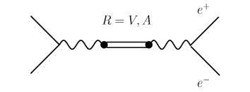
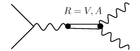
In this section we will consider the Drell-Yan production of resonances leading to , , and three SM gauge boson (, and ) final states. The processes are collected respectively in Fig. 1 and Fig. 2. At the partonic level, the Drell-Yan production of the resonances can be written as
| (17) |
where is the invariant mass of the generic final state and denote the (on-shell) branching ratios of the resonance into initial and final states.
The expression (17) is valid only for close to the resonance peak and neglecting interference effects with SM amplitudes. As we will show, the latter is a good approximation for the leading two and three SM gauge boson final states and relatively light spin-1 masses (up to TeV). On the contrary, interference effects cannot be neglected in the purely leptonic final states.
The convolution with the initial-state parton distribution functions is the same occurring in Drell-Yan processes within the SM (up to tiny higher-order corrections). As a result, it is convenient to normalise the resonant cross sections to SM Drell-Yan processes. To this purpose we define
| (18) |
In the charged case, where we have a single initial state, the situation is particularly simple: using the form factor introduced above the complete cross section for reads
| (19) |
where the explicit expression for the form factor is:
| (20) |
For instance, in the case this implies
| (21) |
with
| (22) |
The large numerical coefficient in (21) and the narrow vector decay width allow us to safely neglect the interference with the SM in this channel, at least up to TeV.
In the neutral case the situation is slightly more complicated by the presence of two basic independent partonic processes. The complete cross section for can be written as
| (23) |
where denote the SM Drell-Yan cross section induced by the partonic process . The explicit expressions for the neutral form factors are:
| (24) |
where
| (25) |
Numerically, , , , .
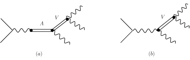
4.1 The three gauge boson final state
The final state with three SM gauge bosons (, , ) is dominated by the intermediate state, with subsequent decay of the heavy vector into a pair of longitudinal gauge bosons. The relevant diagrams are shown in Fig. 2. In this case the pure electroweak SM amplitude is totally negligible, while the relative weight of the resonant processes compared to the non-resonant production depends on the (unknown) mass spectrum of the heavy spin-1 fields. The general structure of the amplitude, taking into account also the non-resonant production, can be written as
| (26) |
where takes into account the off-shell exchange [] and arises by the non-resonant production. Their explicit expressions are
| (27) | |||||
Also in this case the partonic result can easily be translated into the hadronic cross section by means of the form-factor method discussed before. It should be noted that there are always two kinematically independent combinations corresponding to the same three SM gauge boson final state [e.g. and ]. Given the narrow widths of the heavy vectors, to a good approximation we can neglect their interference and sum them incoherently.
5 Numerical analysis
In this section we perform a numerical analysis of the cross sections discussed above for the existing hadron colliders, namely Tevatron ( collisions) and the LHC ( collisions).
We start our analysis with a detailed investigation of the final state. Here we use the recent Tevatron analysis to set bounds on the parameter space of our model. We will also illustrate how this effective approach allows us to easily implement the constraints from electroweak precision observables. We then proceed to discuss the expectations for the LHC in the case of two and three SM gauge boson final states.
5.1 The final state
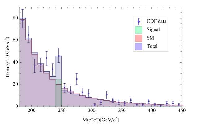
The CDF Collaboration has recently reported the results of a search for high-mass resonances in the spectrum of collisions at 1.96 TeV [14]. This search does not show significant deviations from the SM (with the exception of a excess around GeV, shown in Fig. 3) and can be used to set limits on the parameter space of our model.
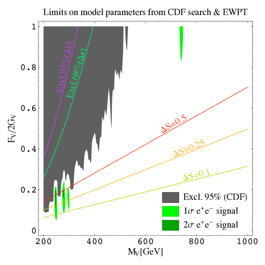
Fitting the CDF spectrum with the SM plus a single vector resonance leads to the exclusion bounds reported in Fig. 4. This analysis has been obtained fixing (from the unitarity constraint), assuming (i.e. neglecting the axial-vector contribution), and taking into account the interference between the SM and the heavy-vector exchange amplitudes. The hadronic cross-section has been obtained using the form-factor method illustrated in Sect. 4, normalizing the results to the published CDF data.
The dark gray area in Fig. 4 denotes the region excluded (at 95% C.L.) by the CDF data. The small green areas correspond to the narrow regions of the parameter space where the deviations from the SM are fitted in terms of the model parameters. Such deviations are not statistically significant yet. However, it is interesting to note that they can be fitted in our model, with values of the free parameters which are not unrealistic (although they are clearly not the most natural ones). In Fig. 4 we also report some EWPO bounds, in particular the contribution of the heavy vector to the parameter
| (28) |
and to the trilinear gauge-boson (TGB) couplings
| (29) |
In the case of we show the result for , which can be considered as the maximal contribution to in this framework. The TGB constraints are obtained neglecting the terms in Eq. (29), a condition which must be fulfilled in any realistic model, given the strong phenomenological constraints on .222 We define trilinear gauge-boson (TGB) couplings and oblique parameters ( and ) as in [15]. On the TGB, following Ref. [16], we impose the constraints and .
As it can be seen in Fig. 4, a light vector resonance could explain the observed excess at GeV. This would not be possible if we impose the hidden-gauge relation , but it can occur in our more general framework, for . Interestingly, the values of and needed to fit such excess are not excluded by EWPO. The positive contribution to need to be partially compensated by a negative from the axial resonance and, most importantly, by a positive . The latter could arise at the one-loop level thanks to the mechanism discussed in [12]: imposing that the axial resonance acts as a cut-off of the one-loop quadratically divergent generated by the light vector field, one obtains
| (30) |
Imposing a good EWPO fit we can thus fully determine the properties of both and states. The axial mass turns out to be determined quite precisely, TeV, providing a simple testable prediction of this framework if the signal in Fig. 4 would become statistically significant.333 An even more stringent prediction is the appearance of an excess similar to the one in Fig. 4 in the spectrum. The absence of significant deviations from the SM in the latter [17] reinforce the explanation of Fig. 4 in terms of statistical fluctuations only.
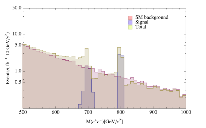
Leaving aside CDF data, in Fig. 5 we show typical signatures of and states in at the LHC for more natural values of their masses. Here the normalization of the cross section and the irreducible SM background has been obtained using Madgraph [18]. In the case of the vector resonance, the signal is obtained for (fixing from unitarity). As it can be seen, even in this favourable case (maximal value of ), the vector peak is hardly visible if GeV. On the other hand, the axial peak could be seen even at larger masses if , leading to a small axial width (see Sect. 3) and a corresponding enhanced peak. The axial signal in Fig. 5 is obtained fixing GeV, GeV, , and (the value of follows from the requirement of a satisfactory EWPO fit).
5.2 Two and three gauge boson final states
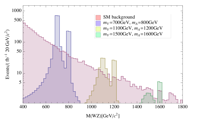
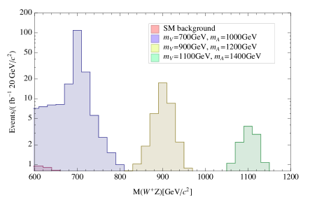
Since the channel is forbidden and the final state represents a difficult experimental signature, in the case of two gauge-boson final states we focus our discussion on the process. In Fig. 6 we show the typical signal at the LHC for the channel for different vector and axial vector masses, assuming a small splitting ( GeV). This plot should be used only for illustrative purposes, given that we have not included the decay branching ratios of and bosons and the corresponding detection efficiencies. As in Fig. 5, the vector signal is obtained for and fixing from unitarity. In order to illustrate the possible contribution of the axial resonances in this channel, we also set , , and . The normalization of the cross section and the irreducible SM background has been obtained using Madgraph [18].
In the three pairs of peaks the first one is always the vector signal. As it can be seen, for and GeV we should expect pairs/, well above the irreducible SM background, or the electroweak cross section for the production of pairs in the SM. A realistic evaluation of the signal efficiency and the corresponding signal/background ratio for this channel is beyond the scope of the present analysis. Here we simply note that using the leptonic () decays of both and bosons leads to a theoretical efficiency of . For and GeV we should thus expect events/ of rather clean leptonic final states, which seems to be a promising signal even with few of integrated luminosity (similar conclusions have indeed been obtained in [11], where a more accurate simulation of this process has been presented).
To a large extent the structure of the vector peak in the channel is model independent: at fixed it can only be rescaled by the ratio (the result obtained for is what is expected in the hidden-gauge models). In Table 1 we report the corresponding cross-sections both at TeV and TeV. For light masses the expected cross sections are close to the present sensitivity of Tevatron for and final states: we have explicitly checked that the recent measurements/bounds on [20] and [19] final states do not pose more stringent bounds on the parameter space of the model with respect to those in Fig. 4.
| GeV | GeV | GeV | |
|---|---|---|---|
| pb | pb | pb | |
| pb | pb | pb |
The axial signal in the channel is subject to a larger uncertainty: for it is a subleading decay mode and there is no hope to observe it; however, for small splitting the axial peak can even exceed the vector one. This is clearly illustrated by the three pairs of peaks in Fig. 6: increasing both and at fixed leads to a reduced relative splitting which enhances the axial signal. It is worth stressing that a small mass splitting between and states is not an unlikely configuration: it is the most simple way to minimize the contribution to , as required by the EWPO.
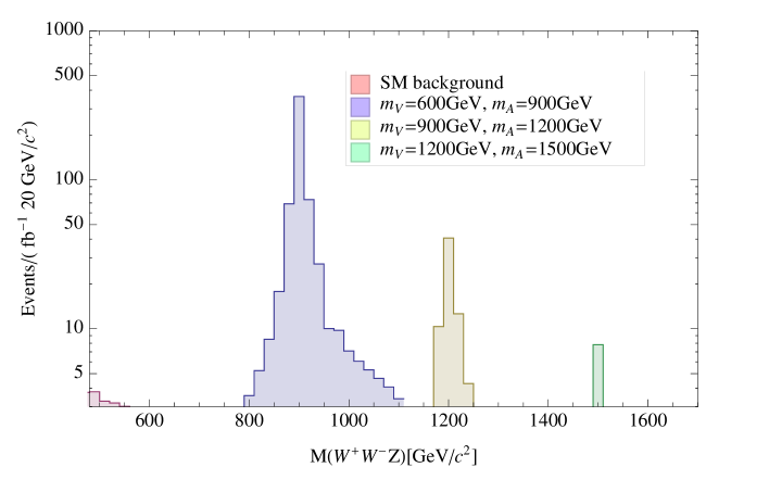
For large mass splittings the dominant axial decay modes are final states with three gauge bosons. In Fig. 7 we show typical signals in the channel. Almost identical distributions are found in the and case. The resonance parameters used for this plots are the same adopted in Fig. 6 with the exception of the masses: a larger mass splitting has been chosen in order to increase the signal. The most interesting observation in this case is that the irreducible SM background is totally negligible, even for large axial masses. Requiring three leptonic decays leads to rather small efficiencies, and it does not necessarily lead to a good rejection of the background for processes with more than one neutrino.444 Requiring at most one neutrino, or zero missing mass, has the double advantage of suppressing the non-irreducible background and allowing the study of the three gauge boson mass spectrum. Generalising the results of Ref. [9] on the case, an efficient background rejection should be obtained requiring two leptonic decays, of which at least one comes from the . According to this strategy, the most promising cases are:
-
•
[] one leptonic , one hadronic , and a leptonic : ;
-
•
[] one leptonic , one leptonic , and one hadronic : .
-
•
[] two leptonic , and one hadronic : .
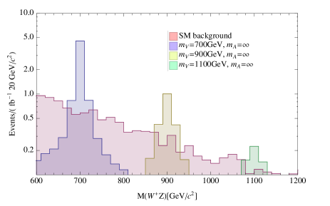
Thanks to the non-resonant diagram in Fig. 2(b), a non-standard signal in the three gauge boson final state could also be obtained in the limit , if were sufficiently light. In such case we would not observe a peak in the three-body mass distribution, but only in specific two-body projections, as illustrated in Fig. 8. A detailed discussion of such signal in the case has been presented in Ref. [9] in the context of the so-called three-site Higgsless model (where there are no light axial-vector resonances). We agree with the conclusion of Ref. [9] that in the three-site Higgsless model the signal is clearly visible at the LHC only with an integrated statistics of . On the other hand, the comparison of the two plots in Fig. 8 shows that in non-minimal models, with relatively light axial vectors, the same signal could be enhanced up to two orders of magnitude, motivating this search even in the early stage of the LHC.
6 Conclusions
Spin-1 resonances are a general feature of Higgsless models: they are typically the lightest non-SM states and play a key role in unitarizing the theory up to a few TeV. The most general signature of these states (in particular of the vector ones, assuming that parity is a good symmetry of the new dynamics), is their appearance in (or ) scattering. This effect is related to the role played by the new states in unitarizing the theory and, to a large extent, it can be predicted in a model-independent way [8]. The only relevant free parameter is the mass of the lightest vector state, which is not fixed by the unitarity condition. As shown by recent analyses (see e.g. [9]), detecting such states in scattering at the LHC is not an easy task: for GeV an integrated statistics of is needed.
In this paper we have analysed the Drell-Yan production (or the production via fusion) of vector and axial-vector states in Higgsless models. Contrary to the fusion, the Drell-Yan production is quite sensitive to the details of the model. We have analysed the problem in general terms using the effective theory approach proposed in Ref. [12], where the relevant properties of the lightest spin-1 states are described in terms of a few effective parameters, and the constraints of EWPO can easily be implemented. Despite the faster drop of the signal/background ratio for rising , compared to fusion, we find that in a large fraction of the parameter space the Drell-Yan production may yield a rather large and clean non-standard signal, even for integrated statistics of . In addition to the mass spectrum, the key parameters here are the effective couplings , which parametrise the (gauge-invariant) mixing of the new states and the SM gauge bosons. Interestingly, the determination of these parameters could shed more light on the role of the resonances in the EWPO [12].
Our main conclusions can be summarised as follows:
-
•
For very light masses ( GeV), the cleanest signal is the final state. In this channel Tevatron is already providing significant constraints in the – plane, that we have summarised in Fig. 4. It is worth stressing that relatively low values are still allowed, provided is not maximal: a configuration which is not allowed in the simplest Higgsless models, but is possible (and even favoured by the EWPO) in our more general effective theory approach.
For large values of (), there are realistic chances to observe deviations from the SM at the LHC, even with a statistics of a few . However, in this channel the signal/background ratio drops very fast with : this implies that it is almost impossible to detect a signal for GeV (even with high statistics). -
•
The final state could offer a wider mass reach, for sufficiently high statistics. Here the starting point are the total cross-sections reported in Table 1. As shown in Fig. 6, the ratio between signal and irreducible background is large even for TeV. Requiring leptonic decays of both and , to suppress the non-irreducible background, the mass region TeV could be explored with an integrated statistics of .
-
•
The and channels are the best channels to search for the axial-vector resonance, if the latter is not degenerate in mass with the vector and is not too heavy. If is large, a configuration which is favoured by the EWPO, the resonance signal in the and channels could be as large as in the case (for similar resonance masses), and would benefit of a smaller irreducible background.
Acknowledgments
We thank Riccardo Barbieri, Roberto Contino, and Vittorio Del Duca for interesting discussions. We are also grateful to Barbara Mele for drawing our attention to the results of Ref. [14]. This work is supported by the EU under contract MTRN-CT-2006-035482 Flavianet.
References
- [1] R. Casalbuoni, S. De Curtis, D. Dominici and R. Gatto, Phys. Lett. B 155 (1985) 95; Nucl. Phys. B 282 (1987) 235.
- [2] C. Csaki et al., Phys. Rev. D 69, 055006 (2004) [arXiv:hep-ph/0305237]; Phys. Rev. Lett. 92 (2004) 101802 [arXiv:hep-ph/0308038].
- [3] Y. Nomura, JHEP 0311 (2003) 050 [arXiv:hep-ph/0309189].
- [4] R. Barbieri, A. Pomarol and R. Rattazzi, Phys. Lett. B 591 (2004) 141 [arXiv:hep-ph/0310285].
- [5] R. Foadi, S. Gopalakrishna and C. Schmidt, JHEP 0403 (2004) 042 [arXiv:hep-ph/0312324].
- [6] H. Georgi, Phys. Rev. D 71 (2005) 015016 [arXiv:hep-ph/0408067].
- [7] R. S. Chivukula, D. A. Dicus, H. J. He and S. Nandi, Phys. Lett. B 562 (2003) 109 [arXiv:hep-ph/0302263].
- [8] J. Bagger et al., Phys. Rev. D 49 (1994) 1246 [arXiv:hep-ph/9306256].
- [9] H. J. He et al., Phys. Rev. D 78 (2008) 031701 [arXiv:0708.2588 [hep-ph]].
- [10] E. Accomando, S. De Curtis, D. Dominici and L. Fedeli, arXiv:0807.5051 [hep-ph]; Nuovo Cim. 123B (2008) 809 [arXiv:0807.2951 [hep-ph]].
- [11] A. Belyaev et al., arXiv:0809.0793 [hep-ph].
- [12] R. Barbieri, G. Isidori, V. S. Rychkov and E. Trincherini, Phys. Rev. D 78 (2008) 036012 [arXiv:0806.1624 [hep-ph]].
- [13] G. Ecker et al., Phys. Lett. B 223 (1989) 425; Nucl. Phys. B 321 (1989) 311.
- [14] T. Aaltonen et al. [CDF Collaboration], Phys. Rev. Lett. 102 (2009) 031801 [arXiv:0810.2059 [hep-ex]].
- [15] T. Appelquist and G. H. Wu, Phys. Rev. D 48 (1993) 3235 [arXiv:hep-ph/9304240].
- [16] S. Dutta, K. Hagiwara, Q. S. Yan and K. Yoshida, Nucl. Phys. B 790 (2008) 111 [arXiv:0705.2277 [hep-ph]].
- [17] T. Aaltonen et al. [CDF Collaboration], arXiv:0811.0053 [hep-ex].
- [18] J. Alwall et al., JHEP 0709 (2007) 028 [arXiv:0706.2334 [hep-ph]], http://madgraph.hep.uiuc.edu/
- [19] T. Aaltonen et al. [The CDF Collaboration], arXiv:0903.0814 [hep-ex].
- [20] V. M. Abazov et al. [D0 Collaboration], arXiv:0904.0673 [hep-ex].