Separating a mixture of chaotic signals

Abstract

Chaos is popularly associated with its property of sensitivity to initial conditions. In this paper we will show that there can be a flip side to this property which is quite fascinating and highly useful in many applications. As a result, we can mix a large number of chaotic signals and one completely arbitrary signal and later a recipient of this transformed and weighted mixture can separate each of the signals, one by one. The chaotic signals, could be generated by various maps which belong to the logistic family. The arbitrary signal, could be a message, some random noise, some periodic signal or a chaotic signal generated by a source, either belonging or not belonging to the family. The key behind this procedure is a family of maps which can dovetail into each other without altering each of their predecessor’s symbolic sequence.

1 Introduction

Chaos is popularly associated with its property of sensitivity to initial conditions. In this paper we will show that there can be a flip side to this property. This side could be found in the case of maps which generate chaotic trajectories. These maps are surjective but not bijective. Therefore there is usually no unambiguous way to go backwards in time. However, if we happen to know the symbolic sequence, reversal is unambiguous. What is more, the conditional reversal maps are contractions and therefore forgiving of errors. This property can be harnessed so that we can mix a large number of chaotic signals and one completely arbitrary signal and later a recipient of this transformed and weighted mixture can separate each of the signals, one by one. In this paper, we will assume that the chaotic signals are generated by various maps which belong to the logistic family. The arbitrary signal, could be a message, some random noise, some periodic signal or a chaotic signal generated by a source, either belonging or not belonging to the family.

The idea behind this study arose soon after a casual discussion in which Professor Walter Freeman Walter made a strong case that the EEG signals are chaotic. Now, if the brain is the command and communication center of the body how could it operate with “chaotic” signals? How do you keep track of which signal came from where?

This paper will now show that the chaotic nature of the signals, instead of being a handicap, is indeed an asset. In fact, today the main motivation for the study of this problem seems be the fact that chaotic maps could be applied to the areas of cryptography, communication and error correction codes (well documented by my colleague Nithin Nagaraj Nithin1 ; Nithin2 ; Nithin3 ). This study has a potential for applications in all these three areas.

In what follows, there is, at first, a review of how various maps can be related using topological conjugacy. Then there is a description of how to create a single noise resistant map. This is followed by ‘a procedure to create a separable cascade of maps which dovetail into each other without altering each of their predecessor’s symbolic sequence. The orbits of these maps can then be mixed at the sender’s end and disentangled at the receiver’s end by using symbolic sequences.

This is followed by a theoretical and numerical demonstration, which begins with $M$ chaotic signals, all generated by the standard tent map, with a random set of initial conditions each, producing $M$ independent chaotic signals of length $L$ each. We then include one more member in this collection which is also of a length $L$. This last signal is quite arbitrary. It could be a message, some random noise, some periodic signal or a chaotic signal generated by a source, either belonging or not belonging to the family. The first $M$ signals naturally have all their terms ranging from 0 to 1. For the last signal, an affine transformation (which is obviously invertible) might be needed to bring its terms within the same range. All the $M+1$ signals are now treated as if they all belonged to the logistic (or the standard tent map) family and each of them is transformed into a different noise resistant map to once again form a separable cascade. The trajectories from these are added and then using a program simulating the receiver, separated and reconstructed into the standard tent map setting. Based on the accuracy specified, a portion of length $Q$ of the tail each signal is abandoned but the $M+1$ sequences of the reduced length $L-Q$ each are highly accurately reproduced by a single message of length $L$.

In a section after the numerical simulation we discuss a scenario which consists of many signals from possibly different maps, (although all belonging to the same conjugate family), coming to a central mixing station. (Please see Figure 1). At this station, each of these signals are transformed to the standard tent map and sent to a receiving station and the receiver upon receiving follows a reversal procedure by which she recovers all the signals with a remarkable accuracy.

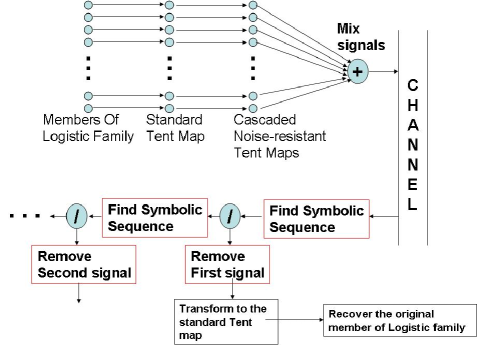
Figure 1: Separating a mixture of chaotic signals.

2 A review of Topological Conjugacy and its use to generate maps which share the same symbolic sequence

Consider a map $U$ that takes $x$ to $U(x)$, that is $x_{n+1}=U(x_{n})$. In order to create a map which is topologically conjugate to this map, we can begin by choosing a function $f$ ,which is continuous with continuous inverse, and using this define $y=f(x)$. From this we can create a new map $V$ which takes $y$ to $V(y)$ by defining $V(y)=f(U(f^{-1}(y)))$. $U$ and $V$ are said to be topologically conjugate.

Such maps share a lot of interesting properties. Of importance for this paper are these two. The first is self evident. If the initial condition of the first map is $x_{0}$, we know that for the second map, the corresponding initial condition would be $y_{0}=f(x_{0})$ and if the first map generates an orbit $x_{0},x_{1},x_{2}...$ we can generate the corresponding orbit $y_{0},y_{1},y_{2},..$ by two different ways: One is to iteratively use $V$ and the other is to operate on the $x$ sequence by $f$. The second property is the preservation of symbolic sequences. Let the domain for $U$ be divided into suitable partitions, known as Markov Partitions, (for the standard tent map below, we choose the symbol 0 if $x$ falls in [0,0.5) and 1 if it falls in [0.5,1] ). Operating $f$ on each of the partitions bijectively maps it into a corresponding partition of $y$. As a result the symbolic sequences for $x$ and $y$ will be identical.

There is a large family of conjugate maps which has the logistic map as one of its most well known members. This family has another key member known as the standard tent map (see below). We would assume in the rest of the paper that the signals to be mixed by the sender are members of this family. We achieve the goal of this paper by creating a new set of members of this family which are parametrized by two parameters $p$ and $q$ and all the members of this new subfamily share an interesting property, described in the next section.

3 Noise resistant sub-family of symbolically equivalent maps

We begin with the standard tent map from [0,1] to [0,1], $T(x):$

$$=2x,~{}~{}~{}x\in[0,0.5),$$

$$=2-2x,~{}~{}~{}x\in[0.5,1].$$

To generate a sub family of maps (see Figure 2) symbolically equivalent to it we choose the transformation $f$ as $y=f(x,p,q)$:

$$=2px,~{}~{}~{}x\in[0,0.5),$$

$$=2px+q,~{}~{}~{}x\in[0.5,1].$$

which leads to a domain for $y$ given by the union of $[0,p)$ and $[p+q,2p+q]$ and we have an inverse transformation $x=f^{-1}(y,p,q)$:

$$=y/2p,~{}~{}~{}y\in[0,p),$$

$$=(y-q)/2p,~{}~{}~{}y\in[p+q,2p+q].$$

Using these two, we get a map $N(y)$ for the variable $y$ from the union of $[0,p)$ and $[p+q,2p+q]$ to itself $N(y)=f(T(f^{-1}(y)))$

This can be explicitly expanded as $N(y):$

$$=2y~{}~{}y\in[0,p/2),$$

$$=2y+q,~{}~{}y\in[p/2,p],$$

$$=4p+3q-2y,~{}~{}y\in[p+q,(3p+2)/q],$$

$$=4p+2q-2y,~{}~{}y\in((3p+2)/q,2p+q].$$

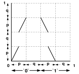
Figure 2: Noise-resistant Tent Map.

Thus the two parameters $p$ and $q$ create a whole subfamily of maps which are topologically conjugate and therefore symbolically equivalent to the standard tent map. For a specific $p$ and $q$ we can define a symbolic sequence corresponding a trajectory generated by $N(y)$ by using the symbol 0 if $x$ is less than $p+q$ and 1 otherwise. This definition helps us embed the domain of the map in a larger interval $[0,2p+2q]$. This extended domain becomes useful when we define an additional variable $z=y+$ an additional signal. Now if the additional signal is non-negative and of a magnitude less than $q$ then it is clear that no matter what $y$ is $z$ will remain in the extended domain.

We will soon make use of the fact that, given a sequence of $y$ and corresponding $z$ , the symbolic sequence of $y$ and $z$ would remain identical.

4 Recovery of signal from a symbolic sequence, in absence of noise

Supposing we start with an initial condition and generate an orbit and also a corresponding symbolic sequence. To what extent can we reconstruct the orbit from the symbolic sequence alone? We would answer this question, first in the absence of noise and then in presence noise or some external signal.

First note that for any allowed combination of p and q the map is surjective but not injective. However, if we are privy to the symbolic sequence, the map becomes invertible. In fact, we can see that $N^{-1}(y,p,q,S)$

$$=y/2~{}~{}~{}if~{}~{}~{}(S=0)\wedge(y<p+(q/2)),$$

$$=(y-q)/2~{}~{}~{}if~{}~{}~{}(S=0)\wedge(y\geq p+(q/2)),$$

$$=2p+q-(y/2)~{}~{}~{}if~{}~{}~{}(S=1)\wedge(y<p+(q/2)),$$

$$=2p+(3q)/2-(y/2)~{}~{}~{}if~{}~{}~{}(S=1)\wedge(y\geq(p+(q/2)).$$

where $S$ is the symbolic sequence entry of the previous point in the orbit.

Please note also that this inverse map contracts any interval to one or two intervals with (total) length of half the original length. So, even if we do not know the end point of the orbit, we could assume two extreme initial conditions and back iterate and after $Q$ steps the orbit is “localized” to a measure of $2^{-Q}$ times the original measure.

Thus the earlier a point in the orbit is, the more accurately is its position determined by the inverse map. This also tells us that if we need to determine all the points of an orbit within an acceptable error of $\epsilon$ for a length of orbit $N$, then we need to run the original calculation for $N+Q$ iterations and supply the symbolic sequence of the whole orbit, where $Q$ has be greater than $-\log_{2}(\epsilon)$.

It should be noted that there is a computationally more efficient way to find the orbit because the family of maps is topologically conjugate to the standard tent map. This implies that for every point on the map there is a corresponding point on the standard map (given by $f^{-1}$ above) which follows an identical symbolic sequence. For the standard map finding an initial condition can be done by reading the symbolic sequence from left to right and repeating it if an even number of 1’s have preceded in the original sequence so far, and “flipping” it (from 0 to 1 or from 1 to 0) if an odd number of 1’s have preceded. The new sequence represents location of the initial condition in binary PGVaidya .

5 Noise resistance

If we add to a sequence $y_{1},y_{2},y_{3}...$ some external signal or noise sequence $r_{1},r_{2},r_{3}...$ and get a new sequence $z_{1},z_{2},z_{3}...$ it is clear that $y$ and $z$ share the same symbolic sequence if $r_{1}$ etc. are non-negative and have a magnitude less than $q$.

Therefore from the symbolic sequence of $z$ we can determine the orbit of $y$ in the same manner and within the same accuracy, as if the noise had no effect on it at all. Thus the entire family of maps is resistant to noise up to a magnitude equal to the parameter $q$.

6 Cascading

We begin with specific values for $p$ and $q$, say $p_{1}$ and $q_{1}$. We select a second set $p_{2}$ and $q_{2}$ so that $q_{1}\geq 2(p_{2}+q_{2}$). Now if we take any two orbits generated by these two maps and add them, it is clear that the sum follows the symbolic sequence of only the first one. Yet, the sum has retained information about both of the sequences because using the symbolic sequence we can determine the first orbit to a predetermined accuracy and then subtract it to get the second orbit.

This process can be continued for a fairly long cascade, each using the noise tolerant corridor of length $q_{n}$ to accommodate the extended diameter of the next stage 2($p_{n+1}+q_{n+1}$) . From a sum of all these signals, starting from the first one all the signals can be recovered one by one, provided we provide sufficient additional length (e. g. $Q$ above) so that the errors in recovery can be regarded as acceptable at each stage.

7 Sender and Receiver

In the next section we will describe numerical results of a simulation in which there is a “sender” who first generates $M$ chaotic signals. All of these are generated using the standard tent map, each of these begin with a randomly chosen initial condition. Each of these $M$ independent chaotic signals are to be of length $L$ each. She then includes a $(M+1)^{st}$ member in this collection which is also of a length $L$. This last signal is quite arbitrary. It could be a message, some random noise, some periodic signal or a chaotic signal generated by a source, either belonging or not belonging to the family. The first $M$ signals naturally have all their terms ranging from 0 to 1. For the last signal, an affine transformation (which is obviously invertible) might be needed to bring its terms within the same range.All the $M+1$ signals are now treated as if they all belonged to the logistic (or the standard tent map) family and each of them is transformed into a different noise resistant map to once again form a separable cascade. The trajectories from these are added and sent to the program simulating the receiver. The receiver also receives the two parameters of the affine transformation, representing scaling and shift. The receiver, then separates and reconstructs the signals into the standard tent map setting. Based on the accuracy specified, the last $Q$ numbers in the tail end of each signal are abandoned. However, the $M+1$ sequences of the reduced length $L-Q$ each are highly accurately reproduced by a single message of length $L$. Thus we have $(M+1)\times(L-Q)$ numbers faithfully carried by L numbers. In our example below $M$ is 20, $L$ is 350 and $Q$ is 50. So signal carried information coding 18 times its length. Chaos is often described by its random like character. If the signals were truly random, this result would be impossible.

8 Numerical verification

We chose $M$ =20 and $L$=350. In generating standard tent map trajectory a modified algorithm was used (please see Appendix 1). We show two extreme cases: 20 chaotic signals (with randomly chosen initial conditions from the standard Tent map) were selected. Some of these signals are seen in Figure 3. These were added to a smooth periodic function which was scaled and a constant was added so that all the terms were from 0 to 1. All these 21 signals were transformed and added. At the recovery stage, for the last signal, the residue after predicting the first 20 signals was chosen. Figures 4a and  4b show the results for the 20th chaotic signal which has the worst fit of all the chaotic signals, yet the recovery is with an error of about $10^{-10}$. Considering that the diameter of the data is close to 1, this is very encouraging. Figures 5a and  5b show the recovery of the periodic signal. The error is of the order of $10^{-4}$. In the next case, another set of 20 chaotic signals are added to a signal which is fully random. In this case, the 20th chaotic signal results (Figures 6a,  6b) are just as good as the first case and the recovery of the random signal (Figures 7a and  7b) has a one order more error than the periodic signal.

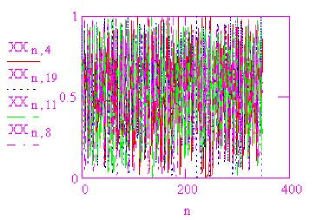
Figure 3: The orbits of the 4 signals out of 20 chaotic signals that will be mixed and separated.

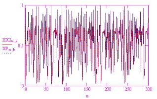
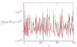
Figure 4: (a) Left: The original (XX2) and the recovered (XP) 20th chaotic signal. (b) Right: The difference of these two signals.

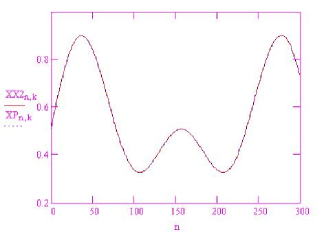
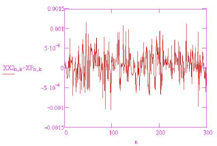
Figure 5: (a) Left: The originally added periodic signal to the mixture and its recovery. (b) Right: The difference between the periodic signal and its recovery.

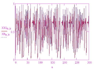
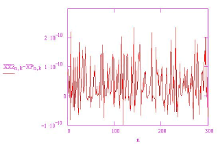
Figure 6: (a) Left: The original (XX2) and the recovered (XP) 20th chaotic signal for the case when added signal is random. (b) Right: The difference between the 20th chaotic signal and its recovery.

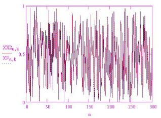
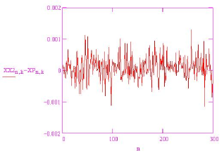
Figure 7: (a) Left: The random signal which was added to the mixture and its recovered signal. (b) Right: Difference between the original and recovered random signal.

9 Extending the possibilities using conjugacies

Now, let us consider a scenario which consists of a central mixing station which receives many signals from possibly different maps, (although all belonging to the same conjugate family, see Figure 1). At this station, each of these signals are transformed to the standard tent map and mixed and then sent to a receiving station and the receiver upon receiving follows a reversal procedure by which she recovers all the signals with a remarkable accuracy. The transformations from the standard tent map to one of its conjugates and their inverses are quite straightforward and well established. However, once this is established a fairly complex problem gets reduced to the one we just simulated above. This opens up possibilities of cryptography, coding and error correction and perhaps begins to explain how the brain might use chaotic signals in its communication system.

10 Conclusions

It has been demonstrated that we can mix a large number of chaotic signals and one completely arbitrary signal and later a recipient of this mixture can separate each of these signals, one by one. This has applications in cryptography and related areas. The paper also helps further understand the nature of chaos.

Appendix

In generating standard tent map trajectory a modified algorithm was used because the tent map has an attractor of 0 (when implemented on a finite precision digital computer which stores and manipulates all numbers in binary) for all initial conditions which can be expanded in a finite number of terms in the binary representation.

The solution is quite simple: we first seek a topologically conjugate map which just represents a scaling by a constant factor: We begin with the standard tent map $T(x)$ which maps [0,1] to [0,1] according to:

$$=2x,~{}~{}~{}x\in[0,0.5R),$$

$$=2R-2x,~{}~{}~{}x\in[0.5R,R].$$

To find a proper trajectory of the standard tent map, the chosen initial condition of the map is multiplied by $R$. Then, one can compute the orbit using the above equation. Once the orbit in the scaled domain is computed, one just divides all the terms of the orbit by $R$ again.

It is important that $R$ should not have a finite binary representation also. When you compare the direct trajectory with the modified trajectory, for the same initial condition, they both remain close for a number of iterations depending on the machine precision and then the conventional trajectory goes to zero. This is because, a computer converts even a so called randomly chosen initial condition into its approximation such that the approximated initial condition has a finite binary representation.

References

- (1) Walter J Freeman, Brain Dynamics: Brain Chaos and Intentionality, Chapter 10b in: Integrative Neuroscience, Bringing Together Biological, Psychological and Clinical Models of the Human Brain Gordon, Evian (ed.)Sydney Australia: Harwood Academic Publishers, 2000. pp. 163-171.
- (2) Nithin Nagaraj, Prabhakar G. Vaidya, and Kishor G. Bhat, Arithmetic Coding as a Non-linear Dynamical System, Communications in Non-linear Science and Numerical Simulation, vol. 14, no. 4, pp. 1013-1020, Apr. 2009. (doi:10.1016/j.cnsns.2007.12.001).
- (3) Nithin Nagaraj, Novel Applications of Chaos Theory to Coding and Cryptography, Ph. D. Thesis, National Institute of Advanced Studies, India 2009 (submitted).
- (4) Nithin Nagaraj, A Dynamical Systems Proof of Kraft-McMillan Inequality and Its Converse for Prefix-free Codes, Chaos 19, 013136, March 2009 (doi:10.1063/1.3080885).
- (5) P. G. Vaidya and V. Kannan, Proof of the existence of Nonergodic Wandering Orbits in the Tent and Related Maps, at 6th International Conference on Difference Equations and Applications, July 30 August 3, 2001, University of Augsburg, Germany.