Shared Information in Stationary States of Stochastic Processes

Abstract

We present four estimators of the shared information (or interdepency) in ground-states given that the coefficients appearing in the wavefunction are all real nonnegative numbers and therefore can be interpreted as probabilities of configurations. Such ground-states of hermitian and non-hermitian Hamiltonians can be given, for example, by superpositions of valence bond states which can describe equilibrium but also stationary states of stochastic models. We consider in detail the last case, the system being a classical not a quantum one. Using analytical and numerical methods we compare the values of the estimators in the directed polymer and the raise and peel models which have massive, conformal invariant and non-conformal invariant massless phases. We show that like in the case of the quantum problem, the estimators verify the area law with logarithmic corrections when phase transitions take place.

As is well known, in quantum mechanics, for a pure state, if ${\cal C=A+B}$ is a bipartition, the von Neumann entanglement entropy $S_{q}$ is defined as

$$S_{q}({\cal A})=S_{q}({\cal B})=-\mbox{Tr}(\rho_{\cal A}\ln\rho_{\cal A})$$ (1)

where $\rho_{\cal A}=\mbox{Tr}_{\cal B}(\rho)$ and $\rho$ is the density matrix related to the ground-state wave function. For one-dimensional spin systems defined by Hermitian Hamiltonians, if the lengths $L$ and $l$ of ${\cal C}$ respectively ${\cal A}$, are large one has the area law ECP . $S_{q}$ stays finite if the correlation length is finite. If the system is gapless and conformal invariant, one gets logarithmic corrections

$$S_{q}(l,L)\sim\gamma\ln l+C\quad(L>>l),$$ (2)

and the finite-size scaling behavior

$$S_{q}(l,L)=\gamma\ln(L\sin{(\pi{l}/{L}})/\pi)+C,$$ (3)

where $\gamma=c/6$ for an open system and $\gamma=2c/6$ for periodic boundary conditions ($c$ is the central charge of the Virasoro algebra) CAR . The factor 2 in the latter case appears because the systems $A$ and $B$ have two common boundaries. $C$ is a non-universal constant. The relations (2)-(3) have been checked analytically and numerically for several models AAA .

In the present paper we consider the shared information (or interdepency) in ground-states which are superpositions of valence bond states. Our considerations apply to ground-states in which the coefficients are all real nonnegative and therefore can be interpreted as probabilities of configurations bravyi . This implies that we consider the shared information resulting from correlations, in a bipartition of a classical and not a quantum system. The ground-states we study can describe equilibrium problems (the spin $1/2$, $SU(2)$ symmetric one dimensional quantum chains RAF ; ASA are an example) but also probability distribution functions (PDF) of stationary states of stochastic processes. We are going to concentrate on the latter and therefore also encounter systems which are scale invariant and not conformal invariant. We will show that if the system is conformal invariant, each entanglement estimator $E(l,L)$ behaves like $S_{q}(l,L)$. The constant $\gamma$ has different values for different estimators. If the system is scale invariant but not conformal invariant, the Eq. (2) stays valid but the finite-size scaling function (3) is different:

$$E(l,L)=\gamma\ln(Lg(l/L)),\quad g(x)=g(1-x),$$ (4)

where $g(x)\sim\alpha x$ for small $x$ and $C=\gamma\ln\alpha$. Like the von Neumann entanglement entropy of quantum systems, the estimators detect the existence of long-range correlations.

We present four estimators of the shared information and compare them considering two models defined using the same configuration space. We give here only the main results, all the details are going to be published elsewhere TBP . Exact results are hard to obtain except for simple cases but for two estimators one can use Monte Carlo simulations for large system sizes and get reliable results. One of the estimators is not new CTW ; ACL ; JLJ , we are going to show its merits and limitations.

In order to define the configuration space, we consider an open one-dimensional system with $L$ sites ($L$ even) connected by $L/2$ non-intersecting links (see Fig. (1)). The links can be seen as $U_{q}(sl(2))$ (a generalization of $SU(2)$ PAS ) singlets. There are $C_{L}=L!/[(L/2)!(L/2+1)!]$ configurations of this kind. There is a bijection between link patterns and restricted solid-on-solid (RSOS) configurations also called Dyck paths. A Dyck path is defined by taking $L+1$ sites situated on the bonds of the link pattern. We attach to each site $i$ non-negative integer heights $h_{i}$ which obey RSOS rules:

$$h_{i+1}-h_{i}=\pm 1,\quad h_{0}=h_{L}=0\quad(i=0,1,\ldots,L).$$ (5)

The height $h_{i}$ represents the number of crossed links at the site $i$ (see Fig. 1). If $h_{j}=0$, at the site $j$ one has a contact point. Between two consecutive contact points one has a cluster. There are four contact points and three clusters in Fig. 1. It is easy to see that for a bipartition, large entanglements take place in large clusters. We present two models. In each of these models one

Figure 1: (Color online) Example of a link pattern for $L=14$ and the corresponding Dyck path. In the latter there are four contact points and three clusters. The shared information is the largest in the left most cluster.

has different probabilities for the various Dyck paths. In the cases in which one considers stationary states of stochastic models, the Dyck paths can be seen as an interface between a substrate ($h_{2i}=0$, $h_{2i-1}=1$, $i=0,1,\ldots,L/2$)) covered by tiles (tilted squares) as shown in Fig. 1 and a gas of tiles (not shown in the figure) GNPR . The PDF of the various Dyck paths are determined by the stochastic process. The latter is defined, in the time-continuous limit, by a non-hermitian Hamiltonian.

We consider the following two models:

A) The directed polymer model (DPM) BEO . A configuration with $m$ contact points gets a factor $K^{m}$ ($K>0$). For $K=1$, all configurations have the same probability $1/C_{L}$ and represent the stationary PDF of the Rouse model ROS of a fluctuating interface. Using reflections about the horizontal axis, one can map the interface onto a random walker problem. The walker starts at the origin and crosses the horizontal axis after $L$ steps. The density of clusters is related to the first passage time problem and vanishes like $L^{-3/2}$ for large $L$. In the whole domain $0<K<2$, one is in the same universality class as for $K=1$. For $K=2$ one gets a surface phase transition and for $K>2$ the density of clusters stays finite in the thermodynamical limit.

B) The stationary states of the raise and peel model (RPM). This is a stochastic model GNPR ; AR in which the adsorption of tiles is local but the desorption is non-local. The model has a free parameter $u$. Typical configurations in the stationary state are shown in Figs.  11 and 15 of Ref. AR . If $0<u<1$, the correlation length is finite and one has finite densities of clusters (see Fig. 12 in AR ). If $u=1$, the average density of clusters vanishes in the thermodynamical limit and the system is conformal invariant (the dynamic critical exponent $z=1$). This property makes the model special. The valence bonds represent $U_{q}(sl(2))$ singlets for $q=\exp(i\pi/3)$. The PDF in the stationary state has also remarkable combinatorial properties. For $u>1$ the system stays critical but conformal invariance is lost. The exponent $z$ decreases smoothly with $u$ from $1$ to zero. There are fewer but larger clusters ALR than for $u=1$. Because of its rich phase diagram, the RPM is an ideal playground to test various estimators.

A bipartition of the system is obtained in the following way. The ensemble of Dyck paths (system $\cal C$ of size $L$ ($L+1$ sites)) is divided into two parts: the sites $0\leq i\leq l$ (part ${\cal A}$) and the sites $l\leq j\leq L$ (part ${\cal B}$). This implies the splitting of each Dyck path which at the site $l$ has the height $h_{l}$ into two ballot paths KSH . One RSOS path which starts at $i=0$ and ends at the site $l$ at the height $h_{l}$ and another one which starts at $i=l$, with height $h_{l}$, and ends at a height zero at $i=L$. We denote by $P(a(h_{l}),b(h_{l}))$ the probability to have a given Dyck path in ${\cal C}$ formed by the ballot paths $a(h_{l})$($b(h_{l})$) in ${\cal A}$, respectively in $B$. We consider the marginals

$$P(a(h_{l}))=\sum_{b}P(a(h_{l}),b(h_{l})),$$ (6)

and $P(b(h_{l}))$. The probability to have a height $h_{l}$ at the site $l$ is

$$F(h_{l})=\sum_{a}P(a(h_{l}))=\sum_{b}P(b(h_{l})).$$ (7)

We present the four estimators. They all measure in different ways the amount of information that can be obtained about the ballot paths in $B$ if one observes the ballot paths in ${\cal A}$.

I) Mutual Information.

$$I(l,L)=-\sum_{h_{l},a(h_{l}),b(h_{l})}P(a(h_{l}),b(h_{l}))\ln{\frac{P(a(h_{l}),b(h_{l}))}{P(a(h_{l}))P(b(h_{l}))}}.$$ (8)

This is a known estimator CTH .

II) Boundary Shannon Entropy

$$S(l,L)=H(L)-H(l)-H(L-l),$$ (9)

where $H(M)=-\sum_{k}P_{k}\ln(P_{k})$ is the Shannon entropy for a system of size $M$ and $P_{k}$ is the probability to have a Dick path $k$. Notice that if, like in model $A$ with $K=1$, all configurations have the same probabilities and their number is $Z(M)$,

$$S(l,L)=-\ln Q(L,l),$$

$$Q(L,l)=Z(l)Z(L-l)/Z(L)=F(h_{l}=0),$$ (10)

where $Q(L,l)$ is the probability to have the two systems ${\cal A}$ and ${\cal B}$ separated by a contact point at the site $l$.

III) Density of Contact Points Estimator

$$D(l,L)=\ln(1/F(h_{l}=0)).$$ (11)

Notice that $D(l,L)$ and $S(l,L)$ coincide if all configurations have the same probabilities. The physical meaning of $D(l,L)$ is simple: if ${\cal A}$ and ${\cal B}$ have a small probability to be separated by a contact point the estimator is large. This should be the case since the shared information among ${\cal A}$ and ${\cal B}$ is large.

In the continuum, $F(h_{l}=0)$ can be replaced by $\rho(l,L)$, the local density of contact points at the distance $l$ from the origin for a system of size $L$. This is an average of a local operator. Let us observe that for $1<<l,L$ the density $\rho$ stays finite, and therefore $D(l,L)$ is also finite. If for large values of $l$ and $L$ one has,

$$\rho(l,L)=1/[Lg(l/L)]^{X},$$ (12)

with $g(x)\sim\alpha x$ for small $x$ ($\alpha$ being a constant), one obtains (2) and (4) with $\gamma=X$. [The average number of clusters is $\rho(L)\sim L^{-X}$.]

IV) Valence Bond Entanglement Entropy.

This estimator was introduced independently by Chhajlany et al CTW and Alet et al ACL and further studied by Jacobsen and Saleur JLJ (see also MMA ). The estimator is the average height at the site $l$, for a system of size $L$:

$$h(l,L)=\sum_{h_{l}}h_{l}F(h_{l}).$$ (13)

We give the main results for the four estimators for each of the two models presented above (see TBP ).

Directed Polymer Model:

It is easy to show that for $K=1$ one has

$$I(l,L) = 1/2\ln(l(L-l)/L)+\gamma_{e}-1/2(\ln(\pi/2)+1)=$$ (14)

$$\sim 1/2\ln(l)+0.303007\quad(L>>l),$$

$$S(l,L) = D(l,L)=\frac{3}{2}\ln(\frac{l(L-l)}{L})+\frac{1}{2}\ln{\frac{\pi}{8}}.$$ (15)

In (14) $\gamma_{e}$ is the Euler constant. Notice that Eq.(2) stays valid, the finite-size scaling functions in (14) and (15) are the same but different from the one given by (3). We have checked TBP that except for the additive constants, Eqs. (14) and (15) are valid in the whole interval $0<K<2$ as expected from universality. The valence bond entanglement entropy does not get logarithmic but power corrections to the area law since $h(l,L)\sim l^{1/2}f(l/L)$ in the whole interval $0<K<2$ BEO . For $K>2$ and large values of $L$, the density of clusters is finite and all estimators verify the area law.

Raise and Peel Model:

${\bf u<1}:$

$D(l,L)$ and $h(l,L)$ are finite since the average density of clusters is finite. $I(l,L)$ and $S(l,L)$ were not computed.

u=1 (conformal invariance):

$I(l,L)$ and $S(l,L)$ are hard to obtain since the PDF is know exactly only for small lattices. Some rough estimates given in TBP show that they are compatible with (3).

$D(l,L)$ is obtained in the following way. As shown in APR in an ”almost” rigorous way, the density of contact points is the average of a local operator of a conformal field theory and has the expression: $\rho(l,L)=m/[L\sin(\pi l/L)]^{1/3}$ where $m=-\sqrt{3}\Gamma(-{1}/{6})/(6\pi^{5/6})$. Using (12) one finds: $D(l,L)=1/3\ln(L\sin(\pi l/L)/\pi)+0.28349.$ This is precisely Eq. (3) in which $\gamma=1/3$ is not given by the central charge of the Virasoro algebra (one would expect $\gamma=1/6$ if this would have been the case) but by the scaling dimensions of a local operator. Moreover one can estimate what would happen if the segment ${\cal A}$ would be inside an infinite system (two separation points). The estimator $D(l,\infty)$ is given by the two-point correlation function of the densities separated by $l$, measured in ALR . One obtains a violation of the area law (2) with $\gamma=2/3$.

$h(l,L)$ was obtained using Monte Carlo simulations for lattices up to $L=9600$. The results are compatible with Eq. (3): $h(l,L)=0.277\ln(L\sin(\pi l/L)/\pi)+0.73$.

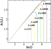
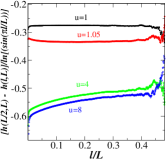
Figure 2: (Color online). Left plot: The estimator $h(l,L)$ for $u=1$ for various lattice sizes L ($l<<L$) as a function of $\ln l$. Right plot: The scaling function $[h(L/2,L)-h(l,L)]$ divided by $\ln(\sin(\pi l/L))$ for various values of $u$ measured on a lattice of size $L=2400$. For $u=1$ one should get a constant independent on $l$.

These results were obtained in the following way. First we have taken $l<<L$ and plotted $h(l,L)$ as a function of $\ln l$ for various values of $L$ (see Fig. 2). One can see that there is a domain where we have a straight line which is $L$ independent. This has allowed to get $\gamma$ and $C$ (see Eq.  (2)).

Next, we have considered the quantity $[h(L/2,L)-h(l,L)]/\ln[\sin(\pi l/L)]$ for various values of $L$. If Eq. (4) is valid one should obtain a constant equal to $-\gamma$. The data are presented in Fig. 2 for $L=2400$ and one can see that this is indeed the case. We should mention that considering periodic boundary conditions and the boundary Coulomb gas formalism, Jacobsen and Saleur JLJ have obtained the value of $\gamma$ (one has to take half of their value since we deal with an open system) $\gamma=\sqrt{3}/2\pi\sim 0.275$ which is compatible with our result. It is remarkable that the two estimators $D(l,L)$ and $h(l,L)$ give values for $\gamma$ which are close to each other.

${\bf u>1}:$

The estimator $D(l,L)$ can be computed using Monte Carlo simulations. A rough estimate of $\gamma$ can be obtained using the equality $\gamma=X$ where the exponent $X$ is related to the density of clusters (see PAS ). The exponent $X$ varies between $1/3$ and $1$ when $u$ increases from $1$ to large values. One has $X=0.5$, $0.6$ and $0.85$ for $u=1.2$, $1.5$ and $10$, respectively ALR .

We have done a more detailed study for $u=4$ ($z\sim 0.3$) in this case and for $D(l,L)$ we found (14) with $\gamma=0.73\pm 0.03$ and a scaling function $g(l/L)$ different of (3) (conformal invariance is lost at $u=4$). We have also studied $h(l,L)$ and found $\gamma=0.63\pm 0.03$ and a function $g(x,L)$ (see right plot of Fig. 2) equal within errors to the one observed for $D(l,L)$ FN1 . Notice that for both estimators the values of $\gamma$ have increased by more than a factor of two as compared with the values observed at $u=1$. An increase of the shared information was expected since there are larger clusters connecting the subsystems ${\cal A}$ and ${\cal B}$.

The estimators defined above can be used for stationary states of other processes not taking place in the Dyck paths configuration space. A simple example is the asymmetric exclusion problem (ASEP) with a density $r$ of particles on a ring of perimeter $L$. The role of the heights in the Dyck paths is played by the deviation of the number of particles in a subsystem (size $l$) from the number $rl$. The system being critical, one expects corrections to the area law. One finds indeed:

$$I(l,L)=S(l,L)=D(l,L)=$$

$$1/2\ln(l(L-l)/L)+1/2\ln(2\pi r(1-r)).$$

Notice that $\gamma$ in (2) is $r$ independent.

We have shown that the four estimators of the shared information between two subsystems, defined above, verify the area law. If the system is gapless, one obtains (with one exception) logarithmic corrections with the coefficient $\gamma$ in (2) increasing if the shared information is larger. The exception is the average height, which in the directed polymer model gets power corrections probably due to the fact that the density of clusters decreases very fast with the size of the system. As a result, the existence of corrections to the area law can be used to detect the existence of phase transitions. Moreover, the observation of a finite-size scaling law like (3) can be an indication of conformal invariance. The estimators presented here have been generalized to the multi-partition case (see [7]).

References

- (1) J. Eisert, M. Cramer and M. B. Plenio, quant-ph:0808.3773.
- (2) P. Calabrese and J. L. Cardy, J. Stat. Mech. P06002 (2004).
- (3) L. Amico, F. Rosario, A. Osterloh and V. Vlatko, Rev. Mod. Phys, 80, 517 (2008) and references therein.
- (4) S. Bravyi, D. P. Di Vincenzo, R. I. Oliveira and B. M. Terhal, quant-ph/0606140; S. Bravyi and B. Terhal, quant-ph/0810.1983
- (5) G. Refael and J. E. Moore, Phys. Rev. Lett. 93, 260602 (2004).
- (6) A. W. Sandvik, Phys. Rev. Lett. 95, 207203 (2005).
- (7) F. C. Alcaraz, V. Rittenberg and G. Sierra, to be published.
- (8) V. Pasquier and H. Saleur, Nucl. Phys. B 330, 523 (1990).
- (9) J. de Gier, B. Nienhuis, P. Pearce and V. Rittenberg, J. Stat. Phys. 114, 1 (2003).
- (10) iA. L OwczareK, J. W. Essam and iR. Brak, J. Stat. Phys. 102, 997 (2001) and references therein.
- (11) P. E. Rouse, J. Chem. Phys. 21, 1272 (1953).
- (12) F. C. Alcaraz and V. Rittenberg, J. Stat. Mech. P07009 (2007).
- (13) F. C. Alcaraz, E. Levine and V. Rittenberg, J. Stat. Mech P08003 (2006).
- (14) K. Shelton, The Singled Out Game, Mathematics Magazine, 78, 15 (2005).
- (15) T. M. Cover and J. A. Thomas, Elements of Information Theory (Wiley, New York) (1991); A. Kraskov, H. Stögbauer and P.Grassberger, cond-mat/0305641.
- (16) R. W. Chhajlany, P. Tomczak and A. Wójcik, Phys. Rev. Lett. 99, 167204 (2007).
- (17) F. Alet, S. Capponi, N. Laflorencie and M. Mambrini, Phys. Rev. Lett. 99, 117204 (2007).
- (18) J. L. Jacobsen and H. Saleur, Phys. Rev. Lett. 100, 087205 (2008).
- (19) M. Mambrini, cond-mat/0706.2508.
- (20) F. C. Alcaraz, P. Pyatov and V. Rittenberg, J. Stat. Mech P01006 (2008).
- (21) For , the average heights of the raise and peel model increase logarithmically with . This point was missed in AR , where the slow logarithmic effects were overlooked and it was claimed that the the heights reach a constant value for large values of .
- (22) R. A. Blythe and M. R. Evans, J. Phys. A 40, R333 (2007).