Abstract

A systematic investigation on vapor-liquid equilibria (VLE) of dipolar and quadrupolar fluids is carried out by molecular simulation to develop a new Helmholtz energy contribution for equations of state (EOS). Twelve two-center Lennard-Jones plus point dipole and point quadrupole model fluids (2CLJDQ) are studied for different reduced dipolar moments $\mu^{*2}=6$, 12, reduced quadrupolar moments $Q^{*2}=2$, 4 and reduced elongations $L^{*}=0$, 0.505, 1. Temperatures cover a wide range from about 55 % to about 95 % of the critical temperature of each fluid. The $N\!pT$ + test particle method is used for the calculation of vapor pressure, saturated densities and saturated enthalpies. Critical data and the acentric factor are obtained from fits to the simulation data. On the basis of this data, an EOS contribution for the dipole-quadrupole cross-interactions of non-spherical molecules is developed. The expression is based on a third-order perturbation theory and the model constants are adjusted to the present 2CLJDQ simulation results. When applied to mixtures, the model is found to be in excellent agreement to results from simulation and experiment. The new EOS contribution is also compatible with segment-based EOS, like the various forms of the Statistical Associating Fluid Theory (SAFT) EOS.

1 Introduction

Knowledge of thermodynamic properties, and in particular vapor-liquid equilibria (VLE), is important for many problems in science and engineering. Among the state-of-the-art thermodynamic models, molecular based approaches have the highest potential to yield significant improvements compared to existing phenomenological approaches, especially in terms of predictive power.

For the two-center Lennard-Jones plus point dipole (2CLJD) fluid and its quadrupolar pendant (2CLJQ), systematic studies of VLE were carried out in previous work [1, 2]. The VLE results were correlated as functions of the model parameters, which were used to determine the model parameters for 78 real fluids [3, 4]. It has been shown that these molecular models can successfully be applied for the description of VLE for binary and ternary mixtures [5, 6, 7]. The simulation data from the two systematic studies [1, 2] were subsequently used to construct equation of state (EOS) contributions due to dipolar [8] and quadrupolar [9] interactions.

As numerous real fluids, e.g., carbon monoxide or refrigerants like R115 (CF₃-CF₂Cl) are both dipolar and quadrupolar, it is valuable to study multipolar model fluids. In case of mixtures, containing dipolar components and quadrupolar components, the polar cross-interaction also plays a significant role. However, only few studies on VLE of fluids that are both dipolar and quadrupolar are available in the literature. Without reference to real fluids, Dubey and O’Shea [10] studied VLE of one-center Lennard-Jones plus dipole and quadrupole model fluids.

Molecular theories for multipolar compounds were developed by Stell et al. [11, 12], based on a perturbation theory around a non-polar reference fluid. A hard-sphere reference was considered by Rushbrooke et al. [13] and later by Henderson et al. [14]. The perturbation theory for mixtures was worked out by Gubbins and Twu [15] considering point-electrostatic multipoles with the spherical Lennard-Jones reference fluid. The perturbation terms were initially parameterized to molecular dynamics results and this parameterization was subsequently improved by Luckas et al. [16]. The perturbation terms were in detail reported by Moser et al. [17] and Shukla et al. [18] and good results were found upon applying that theory to real mixtures [19, 20]. Boublik studied the effect of the non-spherical molecular shape on multipolar interactions, considering the pair correlation function of a Gaussian overlap fluid [21].

An equation of state for the 2CLJD and the 2CLJQ fluid were developed by Saager and Fischer based on molecular simulations. A fixed elongation ($L^{*}=0.505$) was thereby considered and a dipole-dipole term and a quadrupole-quadrupole term were obtained by fitting empirical expressions to the simulation data [22, 23]. Dipole-quadrupole cross-interactions were subsequently treated with an effective one-fluid dipole moment which contains a contribution due to the quadrupole moments of the mixture [24]. Similarily an effective one-fluid quadrupole moment was defined where the dipole moments of components in the mixture contributed according to an empirical relation that was parameterized to simultion data.

Due to the success of the Statistical Associating Fluid Theory (SAFT) EOS [25, 26, 27, 28, 29] in various variants [30, 31, 32, 33, 34, 35], the multipolar terms developed earlier for spherical fluids, were recently applied in combination with different SAFT models [36, 37, 38, 39, 40, 41, 42, 43, 44]. Zhao and McCabe used an integral-equation approach with the mean spherical approximation (MSA) closure in combination with the SAFT-VR EOS [45]. As structural information is available from the MSA term, the orientation of dipoles can be accounted for.

The authors of the present study have recently developed expressions that account for the non-spherical shape of fluids and found good results also for mixtures of 2CLJQ and 2CLJD fluids as well as for mixtures of real substances [8, 9]. Furthermore, Kleiner and Gross [46] accounted for the polarizability of fluids and for the appropriate induction effects of dipoles in applying a renormalization scheme proposed by Wertheim [47, 48, 49, 50]. A combination of the perturbation theory of Moser et al. [17] and of Shukla et al. [18], where the full vectorial and tensorial information of multipoles is utilized, with the approach of our earlier work [8, 9] is presented by Leonhard et al. [51].

In this work, VLE of two-center Lennard-Jones model fluids which are both dipolar and quadrupolar (2CLJDQ) are systematically studied over a wide range of model parameters and temperatures. In reduced units, the 2CLJDQ model class has three molecular parameters that can be varied: elongation, dipole moment and quadrupole moment. Twelve different 2CLJDQ model fluids are covered here. Using these results, an EOS contribution for the dipole-quadrupole cross-interactions of non-spherical molecules is developed based on a third-order perturbation theory. Model constants are thereby adjusted to the simulation results of the 2CLJDQ fluid. Finally, the EOS contribution is compared to experimental and simulation data for five real binary mixtures.

2 Molecular model

The two-center Lennard-Jones plus point dipole and point quadrupole fluids (2CLJDQ) is here investigated. The pair potential of this model class is composed of two identical Lennard-Jones sites a distance $L$ apart (2CLJ) plus a point dipole of moment $\mu$ and a point quadrupole of moment $Q$ placed in the geometric center of the molecule. Both polarities are aligned along the molecular axis. The full potential writes as

$$u_{\rm 2CLJDQ}(\mbox{\boldmath$r$}_{ij},\mbox{\boldmath$\omega$}_{i},\mbox{\boldmath$\omega$}_{j},L,\mu,Q,\sigma,\epsilon) = u_{\rm 2CLJ}(\mbox{\boldmath$r$}_{ij},\mbox{\boldmath$\omega$}_{i},\mbox{\boldmath$\omega$}_{j},L,\sigma,\epsilon)+u_{\rm DD}(\mbox{\boldmath$r$}_{ij},\mbox{\boldmath$\omega$}_{i},\mbox{\boldmath$\omega$}_{j},\mu)$$ (1)

$$+ u_{\rm QQ}(\mbox{\boldmath$r$}_{ij},\mbox{\boldmath$\omega$}_{i},\mbox{\boldmath$\omega$}_{j},Q)+u_{\rm DQ}(\mbox{\boldmath$r$}_{ij},\mbox{\boldmath$\omega$}_{i},\mbox{\boldmath$\omega$}_{j},\mu,Q),$$

where

$$u_{\rm 2CLJ}(\mbox{\boldmath$r$}_{ij},\mbox{\boldmath$\omega$}_{i},\mbox{\boldmath$\omega$}_{j},L,\sigma,\epsilon) = \sum_{a=1}^{2}\sum_{b=1}^{2}4\epsilon\left[\left(\frac{\sigma}{r_{ab}}\right)^{12}-\left(\frac{\sigma}{r_{ab}}\right)^{6}\right],\phantom{0}\phantom{0}\phantom{0}\phantom{0}\phantom{0}$$ (2)

is the Lennard-Jones part. Herein, ${\mbox{\boldmath$r$}}_{ij}$ is the center-center distance vector of two molecules $i$ and $j$, $r_{ab}$ is one of the four Lennard-Jones site-site distances, $a$ counts the two sites of molecule $i$, $b$ counts those of molecule $j$. The vectors ${\mbox{\boldmath$\omega$}}_{i}$ and ${\mbox{\boldmath$\omega$}}_{j}$ represent the orientations of the two molecules. There are three polar contributions, cf. Allen and Tildesley [52]: Firstly, the interaction between dipoles is present

$$u_{\rm DD}(\mbox{\boldmath$r$}_{ij},\mbox{\boldmath$\omega$}_{i},\mbox{\boldmath$\omega$}_{j},\mu) = \frac{\mu^{2}}{\left|\mbox{\boldmath$r$}_{ij}\right|^{3}}\left(s_{i}s_{j}c-2c_{i}c_{j}\right),\phantom{0}\phantom{0}\phantom{0}\phantom{0}\phantom{0}\phantom{0}\phantom{0}\phantom{0}\phantom{0}\phantom{0}\phantom{0}\phantom{0}\phantom{0}\phantom{0}\phantom{0}\phantom{0}\phantom{0}\phantom{0}\phantom{0}\phantom{0}\phantom{0}\phantom{0}\phantom{0}\phantom{0}\phantom{0}\phantom{0}\phantom{0}$$ (3)

secondly, the interaction between quadrupoles

$$u_{\rm QQ}(\mbox{\boldmath$r$}_{ij},\mbox{\boldmath$\omega$}_{i},\mbox{\boldmath$\omega$}_{j},Q) = \frac{3}{4}\frac{Q^{2}}{\left|\mbox{\boldmath$r$}_{ij}\right|^{5}}\left[1-5\left(c_{i}^{2}+c_{j}^{2}\right)-15c_{i}^{2}c_{j}^{2}+2\left(s_{i}s_{j}c-4c_{i}c_{j}\right)^{2}\right],$$ (4)

and finally, the mutual interaction between dipoles and quadrupoles

$$u_{\rm DQ}(\mbox{\boldmath$r$}_{ij},\mbox{\boldmath$\omega$}_{i},\mbox{\boldmath$\omega$}_{j},\mu,Q) = \frac{3}{2}\frac{\mu Q}{\left|\mbox{\boldmath$r$}_{ij}\right|^{4}}\left(c_{i}-c_{j}\right)\left(1+3c_{i}c_{j}-2s_{i}s_{j}c\right),\phantom{0}\phantom{0}\phantom{0}\phantom{0}\phantom{0}\phantom{0}\phantom{0}\phantom{0}\phantom{0}\phantom{0}\phantom{0}\phantom{0}\phantom{0}\phantom{0}\phantom{0}\phantom{0}\phantom{0}$$ (5)

where $c_{k}={\rm cos}\theta_{k}$, $s_{k}={\rm sin}\theta_{k}$, and $c={\rm cos}\phi_{ij}$. $\theta_{i}$ is the angle between the axis of the molecule $i$ and the center-center connection line and $\phi_{ij}$ is the azimuthal angle between the axis of molecule $i$ and $j$. The Lennard-Jones parameters $\sigma$ and $\epsilon$ represent size and energy, respectively.

Among the different spatial arrangements of the four charges in a quadrupole, in 2CLJDQ models they are arranged along the molecular axis in the symmetric sequence $+$, $-$, $-$, $+$ or, having the same energetic effect in pure quadrupolar fluids, $-$, $+$, $+$, $-$. The point quadrupole interaction, cf. Eq. (4), is a large distance approximation, reducing the number of parameters related to the quadrupole to one, namely the quadrupolar moment $Q$. The dipole is approximated in the same sense.

In case of elongated fluids, for very small intermolecular distances $|\mbox{\boldmath$r$}_{ij}|$, the positive Lennard-Jones part $u_{\rm 2CLJ}$ of the full potential cannot outweigh the divergence to $-\infty$ of the polar part $u_{\rm DD}$+$u_{\rm QQ}$+$u_{\rm DQ}$. This divergence of $u_{\rm 2CLJDQ}$ leads to infinite Boltzmann factors, i.e. non-existence of the configurational integral. During molecular dynamics phase space sampling within the pressure range in question, this artifact of the 2CLJDQ potential causes no problem as intermolecular center-center distances are very improbable to fall below critical values. However, during Monte-Carlo simulation or the calculation of entropic properties by test particle insertion [53], critical intermolecular center-center distances might occur. To avoid this problem, following Möller and Fischer [54], a hard sphere of diameter $0.4\sigma$ was placed directly on the polar sites as a shield for critical configurations.

The parameters $\sigma$ and $\epsilon$ were used for the reduction of all thermodynamic properties as well as the model parameters: $T^{*}=Tk_{B}/\epsilon$, $p^{*}=p\sigma^{3}/\epsilon$, $\rho^{*}=\rho\sigma^{3}$, $h^{*}=h/\epsilon$, $L^{*}=L/\sigma$, $\mu^{*2}=\mu^{2}/\left(\epsilon\sigma^{3}\right)$ and $Q^{*2}=Q^{2}/\left(\epsilon\sigma^{5}\right)$. The model parameters were varied in this investigation: $L^{*}=0$, $0.505$ and $1$, $\mu^{*2}=6$ and $12$ as well as $Q^{*2}=2$ and $4$. Combining these values leads to a set of twelve model fluids that were investigated here.

To achieve a monotonous transition from $L^{*}>0$ to $L^{*}=0$, spherical fluids were treated as 2CLJ fluids with $L^{*}=0$. This leads to a site superposition that is not present in the one-center Lennard-Jones case. Therefore, in reduced units, temperature, pressure and enthalpy are fourfold and the squared polar moments twofold of the corresponding values when only one Lennard-Jones site is present. Densities are not affected.

3 Molecular simulation method

Throughout all pure fluid VLE simulations, the $N\!pT$ + test particle method by Möller and Fischer [55, 56] was used. The chemical potential was calculated in the $N\!pT$ ensemble by Widom’s method [53].

In all simulations a center-center cut-off radius $r_{\rm c}=5\sigma$ was used. Outside the cut-off sphere, the fluid was assumed to have no preferential relative orientation of the molecules, i.e. for the calculation of the Lennard-Jones long range corrections, orientational averaging was done with equally weighted relative orientations as proposed by Lustig [57]. Long range corrections for the dipolar interaction were calculated with the reaction field method [58, 22], where the relative permittivity $\epsilon_{\rm s}$ was set to infinity. The quadrupolar interaction needs no long range correction as it disappears by orientational averaging. The same holds for the mixed polar interaction between dipoles and quadrupoles, cf. Weingerl and Fischer [24].

Configuration space sampling was done with $N=864$ particles for both liquid and vapor simulations in the $NpT$ ensemble with Andersons barostat [59]. The reduced integration time step was set to $\Delta t\sqrt{m/\epsilon}/\sigma=0.0015$ and the reduced membrane mass parameter of the barostat was set to $2\cdot 10^{-4}$ for liquid and to $10^{-6}$ for vapor simulations.

Starting from a face centered lattice arrangement, every run was equilibrated over $10,000$ time steps. Data production was performed over $100,000$ time steps. For vapor simulations with $L^{*}=1$, especially those at low temperatures, the Monte-Carlo method was used to achieve equilibrium within an acceptable time range. The number of Monte-Carlo loops was generally chosen to be the same as the number of MD time steps. One Monte Carlo loop is defined here as $N$ trial translations, $\left(2/3\right)N$ trial rotations, and one trial volume change. At each production time step $2N$ test particles were inserted in the liquid phase, and $N$ test particles in the vapor phase to calculate the chemical potential. To get a better accuracy of the chemical potential, $4N$ test particles were used in simulations in the liquid phase at low temperatures.

In some cases, where a highly dense and strongly polar liquid phase was present, the more elaborate gradual insertion scheme had to be employed to obtain the chemical potential sufficiently accurate. The gradual insertion method is an expanded ensemble method [60] based on the Monte Carlo technique. Here, the version proposed by Nezbeda and Kolafa [61] was used, in a form that was extended to the $N\!pT$ ensemble [62]. In comparison to Widom’s test particle method, where whole molecules are inserted in the fluid, gradual insertion introduces one fluctuating molecule, that undergoes changes in a predefined set of discrete states of coupling with the other molecules of the fluid. Preferential sampling is done in the vicinity of the fluctuating particle. This concept leads to considerably improved accuracy of the residual chemical potential. Gradual insertion simulations were performed with $N=864$ particles in the liquid phase. Starting from a face-centered lattice arrangement every simulation run was given $5,000$ Monte Carlo loops to equilibrate. Data production was performed over $100,000$ Monte Carlo loops. Further simulation parameters for runs with gradual insertion were taken from Vrabec et al. [62].

VLE data were determined for temperatures of about 55 % to 95 % of $T^{*}_{\rm c}(\mu^{*2},Q^{*2},L^{*})$. In the whole temperature range all thermodynamic properties of both phases were obtained by simulation.

4 Simulation results of VLE data

Table 1 reports the VLE data of the regarded twelve model fluids. Vapor pressure $p_{\sigma}^{*}$, saturated liquid density $\rho^{\prime*}$, saturated vapor density $\rho^{\prime\prime*}$, residual saturated liquid enthalpy $h^{\prime\mbox{\scriptsize res*}}$ and residual saturated vapor enthalpy $h^{\prime\prime\mbox{\scriptsize res*}}$ are presented, where $h^{\mbox{\scriptsize res*}}=h^{\mbox{\scriptsize*}}(T,p)-h^{\mbox{\scriptsize id}}(T)$. Statistical uncertainties were determined with the method of Fincham et al. [63] and the error propagation law.

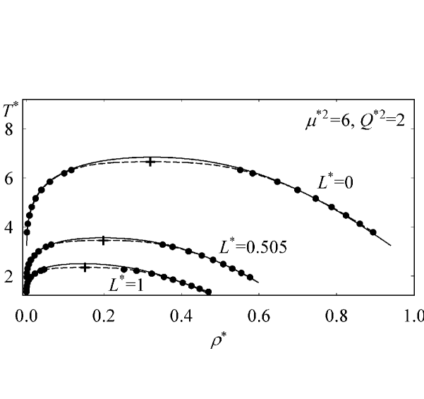
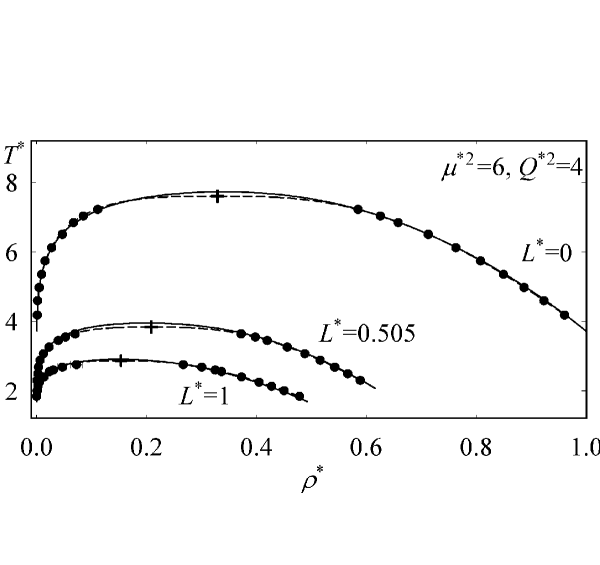
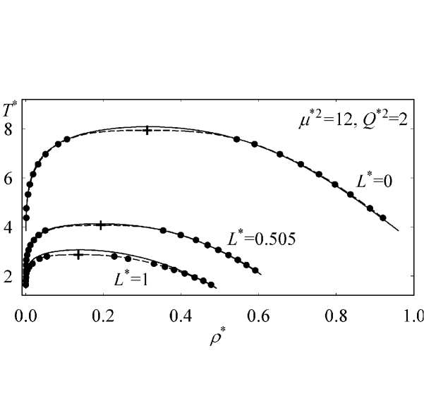
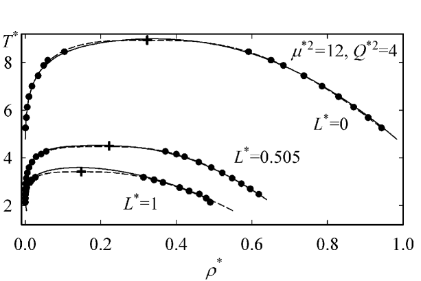
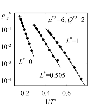
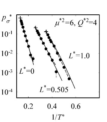
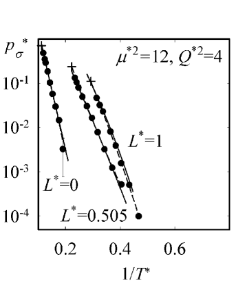
Figs. 1 to 8 illustrate the strong influence of both elongation and polar moments on the VLE data. Elongation and polar moments strongly influence saturated density and the vapor pressure curves. As can be expected, all three critical properties in Figs. 1 to 8, i.e. temperature, density and pressure, decrease with increasing elongation for a given set of polar moments and thus the phase envelopes migrate accordingly. For a constant elongation, they usually increase with increasing polar moments.

To determine the critical data quantitatively, the method of Lotfi et al. [64] was used. The saturated density–temperature dependence near the critical point is well described by $\rho^{*}\sim\left(T^{*}_{\rm c}-T^{*}\right)^{1/3}$, as given by Guggenheim [65, 66]. Therefore, the following correlations were fitted to simulated vapor pressure and saturated densities

$$\ln p^{*}_{\sigma} = c_{1}+\frac{c_{2}}{T^{*}}+\frac{c_{3}}{T^{*4}},$$ (6)

$$\rho^{\prime*} = \rho^{*}_{\rm c}+C_{1}\cdot(T^{*}_{\rm c}-T^{*})^{1/3}+C^{\prime}_{2}\cdot(T^{*}_{\rm c}-T^{*})+C^{\prime}_{3}\cdot(T^{*}_{\rm c}-T^{*})^{3/2},$$ (7)

$$\rho^{\prime\prime*} = \rho^{*}_{\rm c}-C_{1}\cdot(T^{*}_{\rm c}-T^{*})^{1/3}+C^{\prime\prime}_{2}\cdot(T^{*}_{\rm c}-T^{*})+C^{\prime\prime}_{3}\cdot(T^{*}_{\rm c}-T^{*})^{3/2}.$$ (8)

The simultaneous fit of saturated densities, cf. Eqs. (7) and (8), yields $\rho^{*}_{\rm c}$ and $T^{*}_{\rm c}$. Inserting $T^{*}_{\rm c}$ into the vapor pressure fit, cf. Eq. (6), gives the critical pressure $p^{*}_{\rm c}$. These fits can be seen in Figs. 1 to 8. The critical data for the regarded twelve 2CLJDQ model fluids are given numerically in Table 2, which also contains the acentric factor $\omega$

$$\omega\left(\mu^{*2},Q^{*2},L^{*}\right)=-{\rm log}_{10}\frac{p_{\sigma}^{*}\left(\mu^{*2},Q^{*2},L^{*},0.7T^{*}_{\rm c}\right)}{p^{*}_{\rm c}\left(\mu^{*2},Q^{*2},L^{*}\right)}-1,$$ (9)

and the critical compressibility $Z_{\rm c}=p^{*}_{\rm c}/\left(\rho^{*}_{\rm c}T^{*}_{\rm c}\right)$.

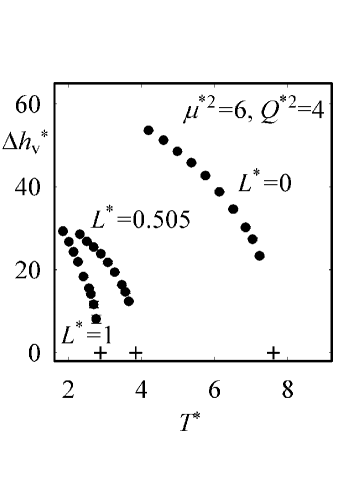
Fig. 9 illustrates the influence of the elongation on the enthalpy of vaporization. An increasing elongation reduces the enthalpy of vaporization. As can be expected (and not shown here), increasing polar moments increase the enthalpy of vaporization.

Thermodynamic consistency of the simulation data was validated with the Clausius-Clapeyron equation

$$\frac{\partial{\rm ln}p_{\sigma}}{\partial T}=\frac{\Delta h_{\rm v}}{p_{\sigma}T\left(1/\rho^{\prime\prime}-1/\rho^{\prime}\right)}.$$ (10)

The vapor pressure correlation, cf. Eq. (6), was used for the left hand side of Eq. (10), while the right hand side was calculated from present simulation data. Within statistical uncertainties, Eq. (10) is fulfilled almost throughout.

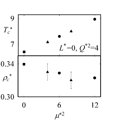
Results from the present study can be compared with other data. Dubey and O’Shea [10] studied VLE of model fluids with both point dipoles and point quadrupoles embedded in one Lennard-Jones site, but unfortunately out of our grid of molecular parameters. In previous work of our group [1], VLE of 2CLJQ model fluids were studied, which is a limiting case here. Fig. 10 presents a comparison of the critical temperature and critical density for different $\mu^{*2}$ for a specified combination of $L^{*}=0$ and $Q^{*2}=4$. It can be seen that present 2CLJDQ data agrees well with the other critical data (including Dubey and O’Shea) [1, 10].

5 Equation of state theory

An EOS for 2CLJDQ fluids can be developed with the help of the VLE simulation results discussed above by applying a perturbation theory following the intermolecular potential, cf. Eqs. (1) and (11). Using the non-polar 2CLJ fluid as a reference fluid, each of the polar contributions to the intermolecular potential, i.e. $u^{DD}$, $u^{QQ}$ and $u^{DQ}$, leads to a perturbation expansion $A^{DD}$, $A^{QQ}$ and $A^{DQ}$ of the Helmholtz energy $A$. The EOS written in the residual Helmholtz energy then reads

$$\frac{A^{res}}{Nk_{B}T}=\frac{A^{2CLJ}}{Nk_{B}T}+\frac{A^{DD}}{Nk_{B}T}+\frac{A^{QQ}}{Nk_{B}T}+\frac{A^{DQ}}{Nk_{B}T},\phantom{0}$$ (11)

where $A^{2CLJ}$ is the residual Helmholtz energy of the 2CLJ reference fluid. The EOS of this reference fluid, $A^{2CLJ}$, can easily be constructed with Wertheim’s Thermodynamic Perturbation Theory of first order (TPT1) [26, 27, 28, 29]. Although the TPT1 initially resulted in a description of tangent-sphere fluids, rather than fused-sphere configurations (such as the 2CLJ model), the TPT1 was shown to form a framework, where the 2CLJ fluid behavior can be recovered with high accuracy. A relation mapping the elongation $L^{*}$ of the 2CLJ fluid to the (noninteger) ”number of tangent-spheres” $m$ was earlier reported [9]. The other parameters of 2CLJDQ fluids, $\sigma$, $\epsilon$, $\mu^{*}$ and $Q^{*}$, also need to be converted to those of the tangent-sphere model. This conversion is straightforward and it is referred to Table 1 of ref. [9]. The superscript ”TS” is used here to indicate parameters of the tangent-sphere model, e.g. it is $\sigma=\sigma^{TS}$. The EOS of the 2CLJ fluid is then

$$\frac{A^{2CLJ}}{Nk_{B}T}=m\cdot\frac{A^{LJ}}{Nk_{B}T}+(1-m)\cdot\ln g^{LJ}(\sigma),$$ (12)

where $g^{LJ}(\sigma)$ is the value of the radial distribution function at the distance $r=\sigma$ as proposed by Johnson et al. [68].

Expressions for $A^{QQ}$ and $A^{DD}$ where reported earlier [9, 8] as third order perturbation expansions written in the Padé approximation. To develop an expression for $A^{DQ}$, an analogous procedure is followed here. The EOS contribution $A^{DQ}$ is presented below for the case of mixtures, since mixtures are considered in section 6. The Helmholtz energy contribution $A^{DQ}$ to Eq. (11) is given as

$$\frac{A^{DQ}}{Nk_{B}T}=\frac{{A_{2}^{DQ}}/{Nk_{B}T}}{1-{A_{3}^{DQ}}/{A_{2}^{DQ}}},\phantom{0}$$ (13)

with $A_{2}^{DQ}$ and $A_{3}^{DQ}$ being the second and third order perturbation terms, respectively. For linear and symmetric molecules, which are considered here, the second order term $A_{2}^{DQ}$ reads in dimensionless form

$$\frac{A_{2}^{DQ}}{Nk_{B}T}=-\frac{9\pi}{4}\rho\sum_{i}\sum_{j}x_{i}x_{j}\frac{\epsilon_{ii}^{TS}}{k_{B}T}\frac{\epsilon_{jj}^{TS}}{k_{B}T}\frac{\sigma_{ii}^{3}\sigma_{jj}^{5}}{\sigma_{ij}^{5}}\mu_{i}^{*TS2}Q_{j}^{*TS2}J_{2,ij}^{DQ},\phantom{0}$$ (14)

where $x_{i}$ is the mole fraction of component $i$, $\mu_{i}^{*TS2}=\mu_{i}^{2}/(m_{i}\epsilon_{ii}^{TS}\sigma_{ii}^{3}$) denotes the dimensionless squared dipole moment in the tangent sphere framwork, and $Q_{i}^{*TS2}=Q_{i}^{2}/(m_{i}\epsilon_{ii}^{TS}\sigma_{ii}^{5}$) the respective dimensionless squared quadrupole moment. The unlike Lennard-Jones parameters $\epsilon_{ij}^{TS}$ and $\sigma_{ij}$ were determined according to the Berthelot-Lorentz combing rules, with $\epsilon_{ij}^{TS}=\left(\epsilon_{i}^{TS}\epsilon_{j}^{TS}\right)^{1/2}$ and $\sigma_{ij}=\left(\sigma_{i}+\sigma_{j}\right)/2$. The abbreviation $J_{2,ij}^{DQ}$ denotes integrals over angles and radius with an integrand being the angle-dependent part of the intermolecular potential weighted with the reference-fluid pair-correlation function. An analytic expression for $J_{2,ij}^{DQ}$ is not easily available and following [8, 9], simple power functions were assumed for $J_{2,ij}^{DQ}$, where the coefficients were adjusted to the present VLE simulation results.

The third order term accounts for three-body effects and consists of two contributions $A_{3}^{DQ}=A_{3}^{DDQ}+A_{3}^{DQQ}$. Similar to $J_{2,ij}^{DQ}$ in the second order term, both terms $A_{3}^{DDQ}$ and $A_{3}^{DQQ}$ contain integrals over the three-body correlation functions. The available data base, including the simulation results of this study, is not sufficiently broad to justify an independent adjustment of expressions for both of these integrals and therefore the third order term is simplified to

$$\frac{A_{3}^{DQ}}{Nk_{B}T}=-\rho^{2}\sum_{i}\sum_{j}\sum_{k}x_{i}x_{j}x_{k}\frac{\epsilon_{ii}^{TS}}{k_{B}T}\frac{\epsilon_{jj}^{TS}}{k_{B}T}\frac{\epsilon_{kk}^{TS}}{k_{B}T}\frac{\sigma_{ii}^{4}\sigma_{jj}^{4}\sigma_{kk}^{4}}{\sigma_{ij}^{2}\sigma_{ik}^{2}\sigma_{jk}^{2}}$$

$$\cdot\left(\mu_{i}^{*TS2}\mu_{j}^{*TS2}Q_{k}^{*TS2}+\alpha\cdot\mu_{i}^{*TS2}Q_{j}^{*TS2}Q_{k}^{*TS2}\right)J_{3,ijk}^{DQ}.$$ (15)

It is thereby assumed that the integrals $J_{3,ijk}$, which appear in both $A_{3}^{DDQ}$ and $A_{3}^{DQQ}$, have a similar density dependence and that the difference between them can be captured by an empirical factor $\alpha$ in Eq. (15). This is certainly a pragmatic approach and may need refinement once a broader data base of simulation results is available. For the integrals $J_{2,ij}^{DQ}$ and $J_{3,ijk}^{DQ}$ simple power functions in density and a rudimentary temperature dependence in the second order term are assumed

$$J_{2,ij}^{DQ} = \sum_{n=0}^{4}\left(a_{n,ij}+b_{n,ij}\frac{\epsilon_{ij}^{TS}}{k_{B}T}\right)\eta^{n},\phantom{0}$$ (16)

$$J_{3,ijk}^{DQ} = \sum_{n=0}^{4}c_{n,ijk}\eta^{n},\phantom{0}$$ (17)

where $\eta$ denotes the packing fraction, which is a dimensionless density. The relation between $\eta$ and $\rho$ depends on the considered EOS, cf. ref. [9]. The coefficients in Eqs. (16) and  (17) depend on the chain length $m$ with

$$a_{n,ij} = a_{0n}+\frac{m_{ij}-1}{m_{ij}}a_{1n}+\frac{m_{ij}-1}{m_{ij}}\frac{m_{ij}-2}{m_{ij}}a_{2n},\phantom{0}$$ (18)

$$b_{n,ij} = b_{0n}+\frac{m_{ij}-1}{m_{ij}}b_{1n}+\frac{m_{ij}-1}{m_{ij}}\frac{m_{ij}-2}{m_{ij}}b_{2n},\phantom{0}$$ (19)

$$c_{n,ijk} = c_{0n}+\frac{m_{ijk}-1}{m_{ijk}}c_{1n},\phantom{0}$$ (20)

and the combining rules of the chain length are given by

$$m_{ij} = \left(m_{i}\cdot m_{j}\right)^{1/2}\phantom{0}$$ (21)

$$m_{ijk} = \left(m_{i}\cdot m_{j}\cdot m_{k}\right)^{1/3}\phantom{0}$$ (22)

The simulation data of vapor pressure and saturated densities given in Table 1 was used to adjust the EOS constants in Eqs. (15) and (18) to (20). The contributions due to the quadrupole-quadrupole interactions and the dipole-dipole interactions needed for optimizing these constants were taken from our earlier studies [8, 9]. Eleven constants, namely $\alpha$ in Eq. (15) as well as $a_{0n}$, $b_{0n}$ and $c_{0n}$ in Eqs. (18) to (20), were adjusted in a first step to the present simulation results for spherical 2CLJDQ fluids, i.e. with $L^{*}=0$. The remaining fifteen constants $a_{1n}$, $a_{2n}$ and $b_{1n}$, $b_{2n}$ and $c_{1n}$ were subsequently adjusted to present simulation results of elongated 2CLJDQ fluids, cf. Table 3.

For the limiting case of non-polar 2CLJ fluids the EOS overpredicts the critical point. During the adjustement of the model constants, the critical point was thus not enforced. A comparison of the EOS to simulation data for saturated liquid and vapor denities is shown in Fig. 1 to 4. Apart from systematic deviations around the critical point, the EOS describes the data with good accuracy. A comparison of the EOS to simulation data for vapor pressures is given in Fig. 5 to 8. Some deviations become apparant for the highest elongation of $L^{*}=1$, while the vapor pressure curves of spherical 2CLJDQ fluids are found to be well described.

6 Application to polar mixtures

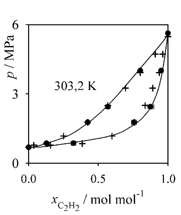
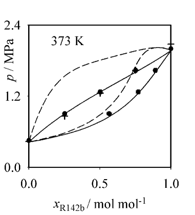
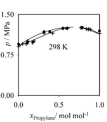
The proposed EOS can readily be applied to mixtures of dipolar and quadrupolar fluids. To assess the capability of the proposed EOS regarding the mixed polar interaction, it was compared to simulative and experimental VLE of the following five binaries: C₂H₂+R152a, R142b+R113, R12+CO₂, R22+R142b and Propylene+R115.

Five of these components are strongly quadrupolar C₂H₂ ($Q=5.1$ DÅ), R113 (13.0 DÅ), Propylene (5.9 DÅ), R115 (9.2 DÅ) and CO₂ (3.8 DÅ) and were modelled by 2CLJQ models in [3, 4]. The numbers in parentheses indicate the polar moment of the molecular model, respectively. The remaining four components R152a ($\mu=2.7$ D), R142b (3.0 D), R22 (2.3 D) and R12 (2.3 D) are dipolar and were modelled by 2CLJD models in [3]. Hence, the first three mixtures mentioned above exhibit the dipole-quadrupole cross-interaction, whereas the remaining two are dipolar or quadrupolar only and are limiting cases here. Simulative VLE calculations were performed on the basis of these molecular models in [69], where one state independent binary parameter $\xi$ for the unlike Lennard-Jones interaction

$$\epsilon_{ij}=\xi\sqrt{\epsilon_{i}\epsilon_{j}}.$$ (23)

was adjusted to one experimental vapor pressure following the procedure proposed in [5]. Table 4 contains the binary parameters derived in [69] and Table 5 compiles the binary VLE data from simulation in numerical form. As can be seen in Figs. 11 to 15, the simulative approach agrees excellently to the experimental data which exhibits in part a qualitatively different phase behavior.

The adopted molecular model (2CLJDQ) is of course simple for the considered real fluids; the most delicate assumptions are: Firstly, the polarizability is not accounted for and vacuum-value dipole moments are used. Secondly, the multipole moments are not represented by (distributed) charges but by point-multipoles. Thirdly, the multipolar moments are assumed to be aligned along the molecular axis. The good agreement of the simulation results to the experimental phase behavior however suggests that important characteristics of the real fluids are captured.

To validate the EOS containing the new dipole-quadrupole contribution, these molecular models were used with exactly the same parameters without any further adjustment. The results are also shown in Figs. 11 to 15. It can be seen that the EOS is in excellent agreement with the simulations, usually within the statistical uncertainty of the simulation data which is often within symbol size. Fig. 12 also gives a comparison with the EOS suggested by Weingerl and Fischer [24]. This model (dotted line) is found in good but not entirely quantitative agreement.

The components of, e.g., the mixture R142b+R113 have high dipole and quadrupole moments, leading to considerable dipole-quadrupole cross-interactions in the mixture. The observation that the EOS predicts the mixture phase behavior well suggests that the polar cross-interactions are adequately captured by the new EOS model. This conclusion is supported by a calculation also shown in Fig. 12, where the dipole-quadrupole cross-iteractions between the two compounds are set to zero. This is done in order to illustrate the contribution that is due to the here proposed expression for $A^{DQ}$. The EOS is for that case (dashed line) not in the vicinity of the data.

7 Conclusion

The VLE of dipolar and quadrupolar two-center Lennard-Jones fluids was studied by molecular simulation to derive a new EOS contribution for the dipole-quadrupole interactions of non-spherical fluids. The vapor pressure, saturated densities and saturated enthalpies were determined with the $N\!pT$ + test particle method applying a gradual insertion scheme in cases of high polar densities. The EOS expression has the form of a perturbation theory of third order where coefficients were adjusted to the bulk properties of the fluids considered in this work. The EOS was subsequently applied to mixtures without adjustable parameters where an excellent agreement to experiment and simulation data was found.

8 Acknowledgment

We gratefully acknowledge financial support by Deutsche Forschungsgemeinschaft, Schwerpunktprogramm 1155. The simulations were performed on the national super computer NEC SX-8 at the High Performance Computing Center Stuttgart (HLRS) under the grant MMHBF.

List of Symbols

Latin alphabet
$a$	equation of state parameter
$a$	interaction site index
$A$	Helmholtz energy
$b$	equation of state parameter
$b$	interaction site index
$c$	equation of state parameter
$c$	coefficient of correlation function
$C$	coefficient of correlation function
$h$	enthalpy
$i$	molecule index
$j$	molecule index
$J$	integral over intermolecular potential
$k_{B}$	Boltzmann constant
$L$	molecular elongation
$m$	chain length
$N$	number of particles
$p$	pressure
$Q$	quadrupolar moment
$r$	site-site distance
$r_{\rm c}$	center-center cut-off radius
$T$	temperature
$u$	pair potential
$x$	mole fraction in the saturated liquid
$y$	mole fraction in the saturated vapor
$Z$	compressibility

Vector properties
$r$	position vector
$\omega$	orientation vector

Greek alphabet
$\alpha$	equation of state parameter
$\Delta h_{\rm v}$	enthalpy of vaporization
$\Delta t$	integration time step
$\epsilon$	Lennard-Jones energy parameter
$\epsilon_{\rm s}$	relative permittivity of dielectric continuum
$\eta$	packing fraction
$\theta$	angle of nutation
$\mu$	dipolar moment
$\rho$	density
$\sigma$	Lennard-Jones size parameter
$\phi_{ij}$	azimuthal angle between the axis of molecules $i$ and $j$
$\omega$	acentric factor

Subscript
c	property at critical point
D	dipole
$i$	component index
$j$	component index
$k$	component index
Q	quadrupole
$\sigma$	vapor-liquid coexistence
2CLJ	two-center Lennard-Jones
2CLJD	two-center Lennard-Jones plus point dipole
2CLJQ	two-center Lennard-Jones plus point quadrupole
2CLJDQ	two-center Lennard-Jones plus point dipole and point quadrupole

Superscript
*	reduced property
′	saturated liquid
′′	saturated vapor
id	ideal gas property
res	residual property
TS	tangent sphere

Table 1: Vapor-liquid equilibrium data of twelve 2CLJDQ model fluids. The number in parentheses indicates the statistical uncertainty in the last decimal digit.

$\!T^{*}$	$p_{\sigma}^{*}$	$\rho^{\prime*}$	$\rho^{\prime\prime*}$	$h^{\prime\mbox{\scriptsize res*}}$	$h^{\prime\prime\mbox{\scriptsize res*}}$
$L^{*}=0$, $\mu^{*2}=6$, $Q^{*2}=2$
3.78268	0.0059 (6)	0.8943 (2)	0.0013 (3)	-42.01 (1)	0.20 (2)
4.12656	0.0152 (9)	0.8510 (2)	0.0038 (3)	-40.38 (1)	-0.50 (2)
4.47044	0.0320 (1)	0.8240 (3)	0.0079 (4)	-38.74 (1)	-1.30 (2)
4.81432	0.0590 (2)	0.7870 (3)	0.0138 (6)	-37.10 (1)	-1.80 (1)
5.15820	0.1040 (2)	0.7463 (4)	0.0237 (6)	-35.35 (2)	-2.60 (7)
5.50208	0.1700 (2)	0.6997 (4)	0.0386 (5)	-33.42 (2)	-3.85 (7)
5.84596	0.2600 (2)	0.6474 (8)	0.0605 (7)	-31.29 (3)	-5.41 (9)
6.18984	0.3810 (3)	0.5840 (1)	0.0970 (2)	-28.74 (5)	-7.80 (2)
6.31849	0.4370 (4)	0.5520 (2)	0.1160 (3)	-27.51 (7)	-8.90 (2)
$L^{*}=0$, $\mu^{*2}=6$, $Q^{*2}=4$
4.18204	0.005 (2)	0.96057 (3)	0.0013 (4)	-54.11 (2)	0 -0.50 (1)
4.59192	0.008 (2)	0.92333 (3)	0.0018 (5)	-51.84 (2)	0 -0.50 (1)
4.97458	0.023 (2)	0.88729 (2)	0.0050 (3)	-49.70 (1)	0 -1.18 (3)
5.35724	0.044 (3)	0.84937 (3)	0.0090 (7)	-47.57 (1)	0 -1.80 (2)
5.73990	0.080 (3)	0.80792 (4)	0.0157 (7)	-45.32 (2)	0 -2.60 (1)
6.12256	0.137 (3)	0.76301 (4)	0.0277 (9)	-42.97 (2)	0 -4.20 (1)
6.50522	0.227 (3)	0.71269 (6)	0.0469 (1)	-40.42 (3)	0 -5.80 (2)
6.84334	0.320 (6)	0.65820 (2)	0.0670 (2)	-37.75 (8)	0 -7.60 (2)
7.03343	0.394 (5)	0.62570 (2)	0.0850 (3)	-36.25 (5)	0 -8.90 (3)
7.22352	0.477 (5)	0.58520 (2)	0.1120 (3)	-34.33 (9)	-11.00 (3)
$L^{*}=0$, $\mu^{*2}=12$, $Q^{*2}=2$
4.36466	0.0049 (5)	0.9208 (3)	0.0012 (1)	-53.68 (1)	0 -0.62 (6)
4.76145	0.0070 (1)	0.8868 (3)	0.0015 (2)	-51.82 (1)	0 -0.60 (1)
5.32623	0.0290 (2)	0.8367 (3)	0.0060 (4)	-49.18 (1)	0 -1.80 (2)
5.73594	0.0520 (2)	0.7971 (3)	0.0102 (4)	-47.19 (2)	0 -2.51 (8)
6.14565	0.0960 (2)	0.7556 (4)	0.0188 (5)	-45.15 (2)	0 -3.90 (1)
6.55536	0.1610 (3)	0.7088 (5)	0.0318 (6)	-42.91 (2)	0 -5.60 (1)
6.96507	0.2490 (3)	0.6550 (7)	0.0509 (9)	-40.41 (3)	0 -7.70 (1)
7.37478	0.3800 (4)	0.5900 (1)	0.0870 (2)	-37.42 (4)	-11.20 (2)
7.53896	0.4320 (4)	0.5540 (2)	0.1000 (2)	-35.81 (8)	-12.10 (2)
7.57963	0.4450 (5)	0.5440 (2)	0.1060 (3)	-35.40 (7)	-12.70 (3)

Table 1: continued.

$\!T^{*}$	$p_{\sigma}^{*}$	$\rho^{\prime*}$	$\rho^{\prime\prime*}$	$h^{\prime\mbox{\scriptsize res*}}$	$h^{\prime\prime\mbox{\scriptsize res*}}$
$L^{*}=0$, $\mu^{*2}=12$, $Q^{*2}=4$
5.25366	0.003 (3)	0.9433 (3)	0.0006 (5)	-63.53 (2)	0 -0.4 (3)
5.69146	0.015 (2)	0.9075 (3)	0.0027 (4)	-61.18 (2)	0 -1.4 (2)
6.12927	0.030 (4)	0.8696 (3)	0.0053 (9)	-58.80 (1)	0 -2.1 (5)
6.56707	0.057 (3)	0.8296 (3)	0.0099 (7)	-56.38 (2)	0 -3.3 (2)
7.00488	0.103 (6)	0.7858 (5)	0.0180 (1)	-53.81 (2)	0 -4.5 (4)
7.44268	0.185 (4)	0.7379 (6)	0.0340 (1)	-51.08 (3)	0 -7.5 (3)
7.88049	0.290 (5)	0.6834 (9)	0.0490 (2)	-48.07 (4)	-10.1 (2)
8.09939	0.347 (6)	0.6510 (1)	0.0600 (4)	-46.33 (4)	-10.9 (6)
8.45000	0.478 (8)	0.5910 (2)	0.1040 (4)	-43.21 (7)	-15.2 (5)
$L^{*}=0.505$, $\mu^{*2}=6$, $Q^{*2}=2$
1.94604	0.0016 (3)	0.5765 (3)	0.0008 (2)	-23.960 (1)	-0.21 (5)
2.12295	0.0028 (5)	0.5542 (3)	0.0014 (2)	-22.960 (1)	-0.30 (4)
2.29986	0.0064 (7)	0.5313 (2)	0.0030 (3)	-21.979 (9)	-0.48 (6)
2.47678	0.0142 (8)	0.5076 (2)	0.0062 (4)	-21.011 (9)	-0.80 (5)
2.65369	0.0260 (2)	0.4816 (6)	0.0113 (9)	-19.990 (2)	-1.30 (1)
2.83060	0.0470 (2)	0.4525 (4)	0.0210 (1)	-18.880 (1)	-2.20 (3)
3.00752	0.0740 (1)	0.4184 (6)	0.0320 (1)	-17.640 (2)	-2.70 (2)
3.18443	0.1100 (1)	0.3770 (1)	0.0500 (1)	-16.200 (4)	-4.00 (2)
3.27289	0.1310 (1)	0.3510 (4)	0.0640 (2)	-15.290 (9)	-4.70 (1)
$L^{*}=0.505$, $\mu^{*2}=6$, $Q^{*2}=4$
2.30000	0.0011 (5)	0.5893 (2)	0.0005 (2)	-28.78 (1)	-0.20 (1)
2.49167	0.0056 (7)	0.5664 (2)	0.0024 (3)	-27.53 (1)	-0.67 (7)
2.68333	0.0090 (2)	0.5426 (3)	0.0037 (9)	-26.30 (1)	-0.83 (2)
2.87500	0.0170 (3)	0.5162 (3)	0.0070 (1)	-25.01 (1)	-1.20 (2)
3.06667	0.0330 (4)	0.4884 (4)	0.0130 (2)	-23.69 (1)	-1.90 (3)
3.25833	0.0580 (2)	0.4562 (4)	0.0230 (1)	-22.25 (2)	-2.80 (1)
3.45000	0.0930 (2)	0.4198 (7)	0.0390 (2)	-20.66 (2)	-4.30 (2)
3.54583	0.1170 (3)	0.3983 (9)	0.0520 (2)	-19.79 (3)	-5.10 (2)
3.64167	0.1430 (2)	0.3720 (1)	0.0700 (2)	-18.77 (4)	-6.40 (1)

Table 1: continued.

$\!T^{*}$	$p_{\sigma}^{*}$	$\rho^{\prime*}$	$\rho^{\prime\prime*}$	$h^{\prime\mbox{\scriptsize res*}}$	$h^{\prime\prime\mbox{\scriptsize res*}}$
$L^{*}=0.505$, $\mu^{*2}=12$, $Q^{*2}=2$
2.23188	0.0011 (3)	0.5917 (2)	0.0005 (2)	-30.816 (9)	-0.63 (9)
2.44569	0.0016 (6)	0.5690 (2)	0.0007 (3)	-29.620 (1)	-0.30 (3)
2.64949	0.0040 (6)	0.5466 (2)	0.0016 (3)	-28.470 (1)	-0.74 (9)
2.85330	0.0093 (9)	0.5226 (3)	0.0036 (4)	-27.330 (1)	-1.20 (2)
3.06000	0.0189 (7)	0.4964 (3)	0.0072 (3)	-26.100 (1)	-1.88 (9)
3.26092	0.0304 (2)	0.4687 (4)	0.0120 (1)	-24.870 (2)	-2.90 (3)
3.46472	0.0550 (1)	0.4384 (5)	0.0213 (6)	-23.570 (2)	-3.76 (9)
3.66853	0.0800 (2)	0.3990 (1)	0.0340 (1)	-21.970 (3)	-5.00 (1)
3.85506	0.1160 (3)	0.3540 (2)	0.0500 (3)	-20.200 (5)	-6.40 (3)
$L^{*}=0.505$, $\mu^{*2}=12$, $Q^{*2}=4$
2.47462	0.00052 (1)	0.6181 (2)	0.00010 (2)	-37.11 (1)	-0.50 (4)
2.69958	0.00124 (1)	0.5958 (2)	0.00034 (5)	-35.67 (1)	-0.10 (2)
2.92455	0.00322 (1)	0.5722 (3)	0.00110 (3)	-34.23 (1)	-1.17 (6)
3.14951	0.00787 (2)	0.5477 (3)	0.00275 (1)	-32.79 (1)	-1.54 (2)
3.37448	0.01649 (8)	0.5214 (3)	0.00562 (5)	-31.32 (1)	-2.22 (3)
3.59944	0.03040 (1)	0.4926 (4)	0.01021 (7)	-29.82 (2)	-3.11 (4)
3.82441	0.04900 (3)	0.4593 (6)	0.01770 (6)	-28.10 (3)	-4.50 (1)
4.04937	0.08000 (4)	0.4220 (1)	0.02900 (3)	-26.29 (4)	-5.80 (5)
4.16186	0.10500 (4)	0.4000 (1)	0.04200 (3)	-25.28 (4)	-7.20 (5)
4.27434	0.13200 (3)	0.3710 (2)	0.05600 (2)	-23.99 (6)	-8.40 (3)
$L^{*}=1$, $\mu^{*2}=6$, $Q^{*2}=2$
1.35000	0.00013 (1)	0.4694 (2)	0.00009 (3)	-23.03 (2)	-0.25 (1)
1.48000	0.00060 (1)	0.4466 (3)	0.00035 (4)	-21.50 (2)	-0.29 (1)
1.60000	0.00187 (3)	0.4257 (3)	0.00126 (5)	-20.22 (2)	-0.56 (6)
1.72000	0.00448 (2)	0.4036 (3)	0.00280 (6)	-18.98 (1)	-0.93 (4)
1.85000	0.00989 (3)	0.3781 (2)	0.00629 (3)	-17.63 (1)	-1.40 (2)
1.96000	0.01775 (7)	0.3549 (3)	0.01138 (6)	-16.50 (1)	-1.93 (1)
2.09000	0.03260 (2)	0.3233 (5)	0.02180 (2)	-15.06 (2)	-2.80 (4)
2.21000	0.05220 (3)	0.2840 (9)	0.03700 (5)	-13.46 (3)	-3.86 (8)
2.26000	0.06270 (4)	0.2510 (2)	0.04560 (7)	-12.35 (5)	-4.34 (9)

Table 1: continued.

$\!T^{*}$	$p_{\sigma}^{*}$	$\rho^{\prime*}$	$\rho^{\prime\prime*}$	$h^{\prime\mbox{\scriptsize res*}}$	$h^{\prime\prime\mbox{\scriptsize res*}}$
$L^{*}=1$, $\mu^{*2}=6$, $Q^{*2}=4$
1.84000	0.0005 (1)	0.4787 (8)	0.00033 (2)	-30.34 (8)	-1.00 (2)
2.00000	0.0019 (1)	0.4505 (3)	0.00100 (2)	-28.14 (2)	-1.38 (9)
2.13000	0.0047 (4)	0.4280 (4)	0.00263 (4)	-26.43 (3)	-2.12 (9)
2.25000	0.0101 (6)	0.4052 (4)	0.00550 (4)	-24.85 (3)	-2.90 (2)
2.40000	0.0238 (3)	0.3731 (4)	0.01360 (4)	-22.79 (2)	-4.40 (2)
2.55000	0.0400 (1)	0.3367 (6)	0.02360 (1)	-20.68 (3)	-5.10 (2)
2.60000	0.0490 (1)	0.3251 (8)	0.03050 (3)	-19.94 (3)	-5.80 (3)
2.68000	0.0650 (5)	0.3000 (1)	0.04700 (8)	-18.70 (4)	-7.10 (8)
2.75000	0.0910 (8)	0.2670 (2)	0.07000 (1)	-17.13 (7)	-9000 (1)
$L^{*}=1$, $\mu^{*2}=12$, $Q^{*2}=2$
1.64000	0.0001 (1)	0.4773 (5)	0.00006 (1)	-30.49 (4)	-1.10 (3)
1.80000	0.0004 (1)	0.4572 (3)	0.00018 (2)	-29.02 (2)	-1.35 (9)
1.94000	0.0011 (1)	0.4350 (3)	0.00065 (1)	-27.31 (3)	-1.76 (5)
2.10000	0.0037 (3)	0.4096 (3)	0.00140 (3)	-25.52 (2)	-2.00 (4)
2.25000	0.0088 (5)	0.3820 (3)	0.00460 (6)	-23.75 (2)	-3.20 (3)
2.37000	0.0148 (1)	0.3588 (4)	0.00853 (9)	-22.36 (2)	-4.03 (4)
2.50000	0.0276 (5)	0.3305 (5)	0.01730 (5)	-20.77 (2)	-5.30 (1)
2.70000	0.0543 (5)	0.2640 (2)	0.03530 (7)	-17.64 (6)	-6.90 (1)
2.80000	0.0730 (1)	0.2280 (3)	0.05400 (1)	-16.01 (9)	-7.90 (1)
$L^{*}=1$, $\mu^{*2}=12$, $Q^{*2}=4$
2.14000	0.00010 (1)	0.4897 (9)	0.00008 (1)	-40.21 (7)	0 -3.20 (3)
2.31000	0.00051 (1)	0.4790 (7)	0.00032 (1)	-39.43 (7)	0 -4.20 (2)
2.48000	0.00157 (2)	0.4610 (1)	0.00082 (3)	-38.00 (1)	0 -4.40 (3)
2.61000	0.00393 (7)	0.4338 (6)	0.00191 (3)	-35.64 (4)	0 -5.56 (5)
2.75000	0.00810 (2)	0.4090 (6)	0.00410 (1)	-33.55 (4)	0 -6.80 (1)
2.97000	0.02300 (1)	0.3646 (6)	0.01250 (9)	-30.24 (3)	0 -8.80 (3)
3.08000	0.03200 (1)	0.3411 (8)	0.01770 (9)	-28.60 (4)	0 -9.40 (2)
3.19000	0.04700 (2)	0.3132 (9)	0.02700 (2)	-26.79 (4)	-10.30 (4)

Table 2: Critical temperature, density, pressure and compressibility as well as acentric factor of twelve 2CLJDQ model fluids.

		$L^{*}$
		$0$		$0.505$		$1$
		$\mu^{*2}$
		$6$	$12$	$6$	$12$	$6$	$12$
$Q^{*2}$		6.651	7.937	3.445	4.067	2.344	2.863	$T^{*}_{\rm c}$
		0.319	0.3128	0.1982	0.1929	0.1508	0.1350	$\rho^{*}_{\rm c}$
	2	0.5995	0.6125	0.1844	0.1692	0.0822	0.0897	$p^{*}_{\rm c}$
		0.2823	0.2467	0.2701	0.2157	0.2324	0.2320	$Z_{\rm c}$
		0.1254	0.1733	0.1987	0.2423	2.4890	2.8628	$\omega$
		7.604	8.944	3.832	4.501	2.861	3.424	$T^{*}_{\rm c}$
		0.3288	0.3229	0.2086	0.1989	0.1532	0.1481	$\rho^{*}_{\rm c}$
	4	0.6797	0.7036	0.2121	0.2382	0.1335	0.1112	$p^{*}_{\rm c}$
		0.2718	0.2436	0.2654	0.2660	0.3045	0.2191	$Z_{\rm c}$
		0.2057	0.2783	0.3296	2.4341	3.2371	3.8008	$\omega$

Table 3: Model constants of the new dipole-quadrupole EOS contribution. In Eq. (15), the parameter $\alpha$=1.19374.

$i$	$a_{0i}$	$a_{1i}$	$a_{2i}$	$b_{0i}$	$b_{1i}$	$b_{2i}$	$c_{0i}$	$c_{1i}$
0	0.6970950	-0.6734593	0.6703408	-0.4840383	0.6765101	-1.1675601	7.846431	-20.72202
1	-0.6335541	-1.4258991	-4.3384718	1.9704055	-3.0138675	2.1348843	33.42700	-58.63904
2	2.9455090	4.1944139	7.2341684	-2.1185727	0.4674266	0	4.689111	-1.764887
3	-1.4670273	1.0266216	0	0	0	0	0	0

Table 4: Binary interaction parameters taken from [69].

Mixture	$\xi$
C2H2+R152a	1.090
R142b+R113	0.952
CO2+R12	0.927
R22+R142b	0.985
Propylene+R115	0.948

Table 5: Vapor-liquid equilibrium data for five binary mixtures taken from [69]. Pure substance vapor pressures were obtained via correlations provided in [1, 2]. The number in parentheses indicates the statistical uncertainty in the last decimal digit.

$x_{1}$ / mol/mol	$p$ / MPa	$y_{1}$ / mol/mol
C2H2+R152a (1+2) at 303.2 K
0	0.69	0
0.128	0.87 (5)	0.320 (2)
0.424	1.77 (5)	0.760 (2)
0.569	2.45 (8)	0.880 (2)
0.801	4.01 (6)	0.950 (4)
1	5.62	1
R142b+R113 (1+2) at 373 K
0	0.45	0
0.252	0.90 (3)	0.570 (2)
0.502	1.27 (4)	0.770 (2)
0.751	1.63 (4)	0.890 (5)
1	2.00	1
CO2+R12 (1+2) at 273 K
0	0.30	0
0.147	0.86 (2)	0.650 (1)
0.388	1.70 (2)	0.849 (6)
0.550	2.20 (2)	0.899 (4)
0.714	2.67 (2)	0.932 (4)
1	3.52	1
R22+R142b (1+2) at 328.15 K
0	0.75	0
0.218	1.02 (1)	0.400 (1)
0.455	1.36 (1)	0.660 (1)
0.560	1.50 (3)	0.730 (8)
0.661	1.66 (2)	0.806 (5)
0.806	1.86 (2)	0.900 (3)
1	2.17	1
Propylene+R115 (1+2) at 298 K
0	0.95	0
0.113	0.98 (4)	0.175 (7)
0.316	1.18 (3)	0.386 (8)
0.549	1.24 (2)	0.590 (1)
0.788	1.26 (2)	0.780 (7)
1	1.19	1

Figure 1: Vrabec and Gross

Figure 2: Vrabec and Gross

Figure 3: Vrabec and Gross

Figure 4: Vrabec and Gross

Figure 5: Vrabec and Gross

Figure 6: Vrabec and Gross

Figure 7: Vrabec and Gross

Figure 8: Vrabec and Gross

Figure 9: Vrabec and Gross

Figure 10: Vrabec and Gross

Figure 11: Vrabec and Gross

Figure 12: Vrabec and Gross

Figure 13: Vrabec and Gross

Figure 14: Vrabec and Gross

Figure 15: Vrabec and Gross

References

- [1] Stoll, J.; Vrabec, J.; Hasse, H.; Fischer, J. Fluid Phase Equilib. 2001, 179, 339.
- [2] Stoll, J.; Vrabec, J.; Hasse, H. Fluid Phase Equilib. 2003, 209, 29.
- [3] Stoll, J.; Vrabec, J.; Hasse, H. J. Chem. Phys. 2003, 119, 11396.
- [4] Vrabec, J.; Stoll, J.; Hasse, H. J. Phys. Chem. B 2001, 105, 12126.
- [5] Stoll, J.; Vrabec, J.; Hasse, H. AIChE J. 2003, 49, 2187.
- [6] Vrabec, J.; Stoll, J.; Hasse, H. Mol. Sim. 2005, 31, 215.
- [7] Stoll, J. Molecular Models for the Prediction of Thermophysical Properties of Pure Fluids and Mixtures; Fortschritt-Berichte VDI, Reihe 3, 836, VDI Verlag: Düsseldorf, 2005.
- [8] Gross, J.; Vrabec, J. AIChE J. 2006, 52, 1194.
- [9] Gross, J. AIChE J. 2005, 51, 2556.
- [10] Dubey, G. S.; O’Shea, S. F. Phys. Rev. E 1994, 49, 2175.
- [11] Stell, G.; Rasaiah, J. C.; Narang, H. Mol. Phys. 1972, 23, 393.
- [12] Stell, G.; Rasaiah, J. C.; Narang, H. Mol. Phys. 1974, 127, 393.
- [13] Rushbrooke, G. S.; Stell, G.; Hoye, J. S. Mol. Phys. 1973, 26, 1199.
- [14] Henderson, D.; Blum, L.; Tani, A. Equation of state of ionic fluids; in: Chao, K. C.; Robinson, R. L.; Eds. Equations of State. Theories and Applications; ACS Symposium Series 300: Washington, DC, American Chemical Society, 1986, p. 281.
- [15] Gubbins, K. E.; Twu, C. H. Chem. Eng. Sci. 1978, 33, 863.
- [16] Luckas, M.; Lucas, K.; Deiters, U.; Gubbins, K. E. Mol. Phys. 1986, 57, 241.
- [17] Moser, B.; Lucas, K.; Gubbins, K. E. Fluid Phase Equilib. 1981, 7, 153.
- [18] Shukla, K. P.; Lucas, K.; Moser, B. Fluid Phase Equilib. 1983, 15, 125.
- [19] Shukla, K. P.; Lucas, K.; Moser, B. Fluid Phase Equilib. 1984, 17, 19.
- [20] Shukla, K. P.; Lucas, K.; Moser, B. Fluid Phase Equilib. 1983, 15, 125.
- [21] Boublik, T. Mol. Phys. 1992, 76, 327.
- [22] Saager, B.; Fischer, J.; Neumann, M. Mol. Sim. 1991, 6, 27.
- [23] Saager, B.; Fischer, J.; Fluid Phase Equilib. 1992, 72, 67
- [24] Weingerl, U.; Fischer, J. Fluid Phase Equilib. 2002, 202, 49.
- [25] Chapman, W. G.; Jackson, G.; Gubbins, K. E. Mol. Phys. 1988, 65, 1057.
- [26] Wertheim, M. S. J. Stat. Phys. 1984, 35, 19.
- [27] Wertheim, M. S. J. Stat. Phys. 1984, 35, 35.
- [28] Wertheim, M. S. J. Stat. Phys. 1986, 42, 459.
- [29] Wertheim, M. S. J. Stat. Phys. 1986, 42, 477.
- [30] Blas, F. J.; Vega, L. F. Ind. Eng. Chem. Res. 1998, 37, 660.
- [31] Blas, F. J.; Vega, L. F. J. Chem. Phys. 1998, 109, 7405.
- [32] Pámies, C. J.; Vega, L. F. Ind. Eng. Chem. Res. 2001, 40, 2532.
- [33] Gil-Villegas, A.; Galindo, A.; Whitehead, P. J.; Mills, S. J.; Jackson, G.; Burgess, A. N. J. Chem. Phys. 1997, 106, 4168.
- [34] Davies, L. A.; Gil-Villegas, A.; Jackson, G. Int. J. Thermophys. 1998, 19, 675.
- [35] Gross, J.; Sadowski, G. Fluid Phase Equilib. 2000, 168, 183.
- [36] Gross, J.; Sadowski, G. Ind. Eng. Chem. Res. 2001, 40, 1244.
- [37] Kraska, T.; Gubbins, K. E. Ind. Eng. Chem. Res. 1996, 35, 4727.
- [38] Jog, P. K.; Chapman, W. G. Mol. Phys. 1999, 97, 307.
- [39] Jog, P. K.; Sauer, S. G.; Blaesing, J.; Chapman, W. G. Ind. Eng. Chem. Res. 2001, 40, 4641.
- [40] Tumakaka, F.; Sadowski, G. Fluid Phase Equilib. 2004, 217, 233.
- [41] Li, X. S.; Lu, J. F.; Li, Y. G.; Liu, J. C. Fluid Phase Equilib. 1998, 153, 215.
- [42] Liu, W. B.; Li, Y. G.; Lu, J. F. Fluid Phase Equilib. 1999, 158, 595.
- [43] Karakatsani, E. K.; Spyriouni, T.; Economou, I. G. AIChE J. 2005, 51, 2328.
- [44] Karakatsani, E. K.; Economou, I. G. J. Phys. Chem. B 2006, 110, 9252.
- [45] Zhao, H. G.; McCabe, C. J. Chem. Phys. 2006, 125, 104504.
- [46] Kleiner, M.; Gross, J. AIChE J. 2005, 51, 2556.
- [47] Wertheim, M. S. Mol. Phys. 1977, 35, 1109.
- [48] Wertheim, M. S. Mol. Phys. 1979, 37, 83.
- [49] Wertheim, M. S. Annu. Rev. Phys. Chem. 1979, 30, 471.
- [50] Gray, C. G.; Joslin, C. G.; Venkatasubramanian, V.; Gubbins, K. E. Mol. Phys. 1985, 54, 1129.
- [51] Leonhard, K.; Nguyen, V. N.; Lucas, K. Fluid Phase Equilib. (Submitted, 2007)
- [52] Allen, M. P.; Tildesley, D. J. Computer Simulation of Liquids; Clarendon Press: Oxford, 1987.
- [53] Widom, B. J. Chem. Phys. 1963, 39, 2808.
- [54] Möller, D.; Fischer, J. Fluid Phase Equilib. 1994, 100, 35.
- [55] Möller, D.; Fischer, J. Mol. Phys. 1990, 69, 463.
- [56] Möller, D.; Fischer, J. Mol. Phys. 1992, 75, 1461.
- [57] Lustig, R. Mol. Phys. 1988, 65, 175.
- [58] Barker, J. A.; Watts, R. O. Mol. Phys. 1973, 26, 789.
- [59] Andersen, H. C. J. Chem. Phys. 1980, 72, 2384.
- [60] Shevkunov, S. V.; Martinovski, A. A.; Vorontsov-Velyaminov, P. N. High Temp. Phys. (USSR) 1988, 26, 246.
- [61] Nezbeda, I.; Kolafa, J. Mol. Sim. 1991, 5, 391.
- [62] Vrabec, J.; Kettler, M.; Hasse, H. Chem. Phys. Lett. 2002, 356, 431.
- [63] Fincham, D.; Quirke, N.; Tildesley, D. J. J. Chem. Phys. 1986, 84, 4535.
- [64] Lotfi, A.; Vrabec, J.; Fischer, J. Mol. Phys. 1992, 76, 1319.
- [65] Guggenheim, E. A. J. Chem. Phys. 1945, 13, 253.
- [66] Rowlinson, J. S. Liquids and Liquid Mixtures; Butterworth: London, 1969.
- [67] Lisal, M.; Aim, K.; Mecke, M.; Fischer, J. Int. J. Thermophys. 2004, 25, 159.
- [68] Johnson, K.; Müller, E. A.; Gubbins, K. E. J. Phys. Chem. 1994, 98, 6413.
- [69] Huang, Y.-L. Vapor-liquid equilibria of polar mixtures by molecular simulation, MSc Thesis, University of Stuttgart, 2005.
- [70] Lim, J. S.; Lee, Y.-W.; Kim, J.-D.; Lee, Y. Y. J. Chem. Eng. Data 1996, 41, 1168.
- [71] Laugier, S.; Richon, D.; Renon, H. Fluid Phase Equilib. 1994, 93, 297.
- [72] Lavrenchenko, G. K.; Nikolovsky, V. A.; Baklai, O. V. Kholod. Tekh. 1983, 6, 41.
- [73] Cao W., Yu H., Wang W. J. Chem. Ind. Eng. (China) 1997, 48, 136.
- [74] Kleiber, M. Fluid Phase Equilib. 1994, 92, 149.