The Dynamical and Chemical Evolution of Dwarf Spheroidal Galaxies

We present a large sample of fully self-consistent hydrodynamical Nbody/Tree-SPH simulations of isolated dwarf spheroidal galaxies (dSphs). It has enabled us to identify the key physical parameters and mechanisms at the origin of the observed variety in the Local Group dSph properties. The initial total mass (gas + dark matter) of these galaxies is the main driver of their evolution. Star formation (SF) occurs in series of short bursts. In massive systems, the very short intervals between the SF peaks mimic a continuous star formation rate, while less massive systems exhibit well separated SF bursts, as identified observationally. The delay between the SF events is controlled by the gas cooling time dependence on galaxy mass. The observed global scaling relations, luminosity-mass and luminosity-metallicity, are reproduced with low scatter. We take advantage of the unprecedentedly large sample size and data homogeneity of the ESO Large Programme DART, and add to it a few independent studies, to constrain the star formation history of five Milky Way dSphs, Sextans, LeoII, Carina, Sculptor and Fornax. For the first time, [Mg/Fe] vs [Fe/H] diagrams derived from high-resolution spectroscopy of hundreds of individual stars are confronted with model predictions. We find that the diversity in dSph properties may well result from intrinsic evolution. We note, however, that the presence of gas in the final state of our simulations, of the order of what is observed in dwarf irregulars, calls for removal by external processes.

1 Introduction

Understanding the dominant physical processes at the origin of the dynamical and chemical properties of dwarf spheroidal galaxies (dSphs) is challenging. The binding energy of the interstellar medium of these low mass systems, at the faint end of the galaxy luminosity function, is weak. The injection of energy, due to violent explosions of supernovae (Dekel & Silk, 1986; Mori et al., 1997; Mac Low & Ferrara, 1999; Murakami & Babul, 1999; Mori et al., 2002; Hensler et al., 2004; Ricotti & Gnedin, 2005; Kawata et al., 2006), or the cosmic UV background during reionization (Efstathiou, 1992; Barkana & Loeb, 1999; Bullock et al., 2000; Mayer et al., 2006) may leave dSphs totally devoid of gas and consequently quench their star formation. In this picture, the majority of the dSphs are fossils of the reionization epoch and are characterized by an old stellar population (Ricotti & Gnedin, 2005).

However, observations offer evidence for more complex star formation histories and reveal a clear variety of dwarf galactic systems (Mateo, 1998; Dolphin, 2002). The spread in stellar chemical abundances, and in particular the low [$\alpha$/Fe] values compared to Galactic halo stars at equal metallicity, are hardly compatible with an early termination of star formation at the epoch of reionization (e.g., Harbeck et al., 2001; Shetrone et al., 1998, 2001, 2003; Tolstoy et al., 2003; Geisler et al., 2005; Koch et al., 2008, examples taken in relation to the galaxies studied in this work). Whilst some dSphs are indeed consistent with rather short star formation episodes, such as Sextans (Lee et al., 2003) or Sculptor (Babusiaux et al., 2005), others are characterized by much more extended periods, like Carina (Smecker-Hane et al., 1996; Hurley-Keller et al., 1998) or Fornax (Coleman & de Jong, 2008).

Long durations of the star formation were early advocated by purely chemical evolution models constrained by the dwarf metallicity distributions and color-magnitude diagrams (Ikuta & Arimoto, 2002; Lanfranchi & Matteucci, 2004). Subsequent simulations of dwarf galaxies introduced the role of the dark matter coupled to the stellar feedback (Ferrara & Tolstoy, 2000), and later the full dynamical physics of the gas and dark matter, by means of N-Body+SPH treatment. Along this line, Marcolini et al. (2006, 2008) concluded that a prolonged (compared to instantaneous) star formation requires an external cause for gas removal, which cannot be due to galactic winds. Intermittent episodes of star formation were at the focal point of the analysis by Stinson et al. (2007). They naturally arose from the alternation between feedback and cooling of the systems. Valcke et al. (2008) confirmed their self-regulated form. These authors also found a gradual shift of the star formation towards the inner galactic regions. Kawata et al. (2006) had looked for evidence of spatial variation as well, in the form of metallicity gradients, but had to stop their simulations at redshift 1. Likewise, considering a cosmological box as initial conditions instead of individual halos, Read et al. (2006) stopped their simulations early, and focused on the smallest and most metal-poor dwarf galaxies.

In all these works, gas remains at the end of the dSph evolutions. The resolution of this problem constitutes a challenge. Mayer et al. (2006) performed simulations of gas-rich dwarf galaxy satellites orbiting within a Milky Way-sized halo and studied the combined effects of tides and ram pressure. They showed that while tidal stirring produces objects whose stellar structure and kinematics resemble that of dSphs, ram-pressure stripping is needed to entirely remove their gas. Salvadori et al. (2008) proposed a semi-analytical treatment in a hierarchical galaxy formation framework and achieved the smallest final gas fraction.

Despite real limitations, such as scarce comparisons with observations, incomplete time-evolution, or ad hoc parameterizations, we are witnessing a rapid convergence toward understanding the formation and evolution of dSphs. A critical step forward must be undertaken with a large set of simulations to be confronted with an equally broad sample of data. In particular, the chemical imprints resulting from different hypotheses have not yet been fully capitalized on.

The VLT/FLAMES instrument, with fiber links to the GIRAFFE and UVES spectrographs, has enabled a revolution in spectroscopic studies of resolved stellar populations in nearby galaxies. It is now possible to measure the abundances of a wealth of chemical elements for more than 100 stars at once. Our ESO-Large Programme DART (Dwarf Abundances and Radial velocity Team) is dedicated to the measure of abundances and velocities for several hundred individual stars in a sample of three nearby dSph galaxies: Sculptor, Fornax, and Sextans. We have used the VLT/FLAMES facility in the low resolution mode to obtain CaII triplet metallicity estimates, as well as accurate radial velocities out to the galaxies’ tidal radii (Tolstoy et al., 2004; Battaglia et al., 2006; Helmi et al., 2006; Battaglia et al., 2008a, b). Each of the three galaxies has also been observed at high resolution for about 80 stars in their central regions, to obtain detailed abundances for a range of interesting elements such as Mg, Ca, O, Ti, Na, Eu. (Venn & Hill, 2005; Letarte et al., 2007, Hill et al in preparation; Letarte et al. in preparation).

In the following, we take advantage of the statistically significant DART sample and data homogeneity, and include some recent independent studies, to constrain the star formation history of five Milky Way dSphs, Sextans, LeoII, Carina, Sculptor, and Fornax. For the first time, populated [$\alpha$/Fe] vs [Fe/H] diagrams can be confronted with model predictions. Our first goal is to establish how well one can reproduce the apparent diversity of dSph star formation histories in a common scheme. We choose to model galaxies in isolation, as this is the only way to control the effect of all parameters at play, and to understand the dominant physical processes. We will try to see if a complex star formation history may result from intrinsic evolution or if external processes are necessary. We have performed an unprecedentedly large number of simulations. Not only do they account for the gravity of the dark matter and baryons, but they also contain a large number of additional physical mechanisms: metal-dependent gas cooling above and below $10^{4}\,\rm{K}$, star formation, SNIa and SNII energy feedback and chemical evolution. We focus on the luminosity, star formation history and metallicity properties of dSphs, rather than on their dynamical properties, which turn out to be less constraining.

The paper is organized as follows: The code and the implementation of physical processes are described in Section 2. The initial conditions are detailed in Section 3. The presentation of the results is split in three parts: Section 4 focuses on the global evolution of the galaxies and discusses the main driving parameters, while Section 5 is devoted to the scaling relations. The detailed analysis of the chemical properties of Sextans, Leo II, Carina, Sculptor, and Fornax are treated in Section 6. Section  7 offers a physical interpretation of the results. Section 8 summarizes our work.

2 The code

We have adapted the code treeAsph originally developed by Serna et al. (1996), with further developments presented in Alimi et al. (2003). The chemical evolution was introduced by Poirier et al. (2003, Poirier, PhD thesis) and Poirier et al. (2002). For the sake of simplicity, we recall below the main features and the general philosophy of the algorithms.

2.1 Dynamics

All gravitational forces are computed under the tree algorithm proposed by Barnes & Hut (1986) (see also Hernquist, 1987). This technique is based on a hierarchical subdivision of space into cubic cells. One approximates the forces due to a cluster of particles contained in a cubic cell and acting on a particle $i$ by a quadrupolar expansion of the cluster gravitational potential. This is done under the condition that the size of the cubic cell is small compared to its distance to the particle $i$. The ratio between size and distance must be smaller than a tolerance parameter, $\theta$, fixed to 0.7 in our simulations (Hernquist, 1987). Indeed, under this condition, the internal distribution of the particles within cells can be neglected. Consequently, the number of operations needed to compute the gravitational forces between $N$ particles scales as $\sim N\log N$, instead of $\sim N^{2}$ if one were to consider each individual pair of particles.

The hydrodynamics of the gas is followed in the Lagrangian Smooth Particle Hydrodynamics (SPH) scheme. Its allows to describe an arbitrarily shaped continuous medium with a finite number of particles (Lucy, 1977; Gingold & Monaghan, 1977), see Monaghan (1992) and Price (2005) for reviews. Each gas particle has its mass spatially smeared out by a smoothing kernel $W$ (here a spline function).

Unlike the gravitational forces, which are determined from the interactions with all other particles in the system, the hydrodynamical forces result from the contributions of a modest number of neighbors. The spatial resolution is determined by the smoothing length $h_{i}$ associated with the particle $i$, computed through the requirement that a sphere of radius $h_{i}$ centered on particle $i$ contains $32$ neighbors.

The integration scheme is the symplectic leapfrog used with adaptative time-steps.

2.2 Cooling

At temperatures lower than $10^{4}\,\rm{K}$, cooling in primordial gas is dominated by the molecule $H_{2}$. Galli & Palla (1998) have shown that the cooling efficiency of $H_{2}$ is determined by its mass fraction $\chi_{H_{2}}$. Unfortunately, an accurate computation of $\chi_{H_{2}}$ is difficult and requires to take into account the complex processes of the formation and destruction of $H_{2}$. Following Maio et al. (2007), we instead fix $\chi_{H_{2}}$to $10^{-5}$. Once the gas is enriched with metals, these are important to the cooling properties. We consider oxygen, carbon, silicon and iron (Maio et al., 2007), since they are the most-abundant heavy atoms released during stellar evolution, particularly by the SNe II and SNe Ia, that we follow in our simulations. We set the density of the free electrons over that of hydrogen , ($n_{\rm{e}^{-}}/n_{\rm{H}}$) to $10^{-4}\,\rm{cm^{-3}}$.

Above $10^{4}\,\rm{K}$, the cooling function is calculated following the metallicity dependent prescription of Sutherland & Dopita (1993). The full normalized cooling function is shown in Figure 1, for a large range of metallicities.

Figure 1: Normalized cooling function as a function of temperature and metallicity.

A more detailed modeling of the gas cooling is not necessary, as long as simulations are limited in spatial resolution. Indeed, the cooling of the gas is directly dependent on its density. Therefore, a limited resolution smoothes the density fluctuations of the interstellar medium.

2.3 Chemical evolution and stellar feedback

The chemical enrichment of the interstellar medium (ISM) depends on the interplay between different physical processes. It requires us to follow the rate at which stars form, the amount of newly synthesized chemical elements, the mass and energy released during the different stellar phases, and, finally, the mixing of the metal-enriched stellar outflows with the ISM. The computation of this cycle is done by implementing the original equations of chemical evolution formalized by Tinsley (1980), as closely as possible.

2.4 Star formation

We adopt the now classical recipe of Katz (1992) and Katz et al. (1996). A gas particle becomes eligible for star formation if it is i) collapsing (negative velocity divergence) and ii) its density is higher than a threshold of $\rho_{\rm{sfr}}=1.67\times 10^{-25}\rm{g/cm^{3}}$. However, we do not require the dynamical time to be shorter than the sound crossing time (Jeans instability).

The gas particles, which satisfy the above criteria, form stars at a rate expressed by:

$$\frac{d\rho_{\star}}{dt}=\frac{c_{\star}}{t_{\rm{g}}}\rho_{\rm{g}},$$ (1)

which mimics a Schmidt law (Schmidt, 1959). $c_{\star}$ is the dimensionless star formation parameter, $t_{\rm{g}}$ is taken as the maximum of the local cooling time and the free-fall time.

For a given time interval $\Delta t$, a gas particle of mass $m_{\rm{g}}$ has a probability $p_{\star}$ to form a stellar particle of mass $m_{\star}$, where $p_{\star}$ is defined by:

$$p_{\star}=\frac{m_{\rm{g}}}{m_{\star}}\left[1-\exp\left(-\frac{c_{\star}}{t_{\rm{g}}}\Delta t\right)\right].$$ (2)

The new stellar particle is initially assigned the position and velocity of its gas progenitor. Subsequently, gas and stellar velocities are modified in order to conserve both energy and momentum.

Each stellar particle represent a cluster of stars, sharing the same age and metallicity, whose initial mass function (IMF) $\Phi(m)$ is described by a Salpeter law (Salpeter, 1955):

$$\Phi(m)=\left[\frac{x+1}{m_{u}^{x+1}-m_{l}^{x+1}}\right]m^{x},$$ (3)

with $x=-1.35$, $m_{l}=0.05\,\rm{M_{\odot}}$ and $m_{u}=50\,\rm{M_{\odot}}$.

2.5 Ejecta

We neglect stellar winds, since they contribute little to the evolution of the chemical elements that we consider (magnesium and iron), and because the injection power to the ISM is dominated by SN explosions (Leitherer et al., 1992).

The amount of energy, mass and metals ejected by a stellar particle during a time interval $\Delta t$ is calculated by considering the mass of stars exploding between $t$ and $t+\Delta t$. The dependency of the stellar lifetimes on metallicity is taken into account following Kodama & Arimoto (1997, private communication).

Hence, the feedback energy released by a stellar particle in the time interval $[t,t+\Delta t]$ is:

$$\Delta E_{\rm{SN}}=m_{\star,0}\,\,\left[n_{\rm{II}}(t)\,E_{\rm{II}}+n_{\rm{Ia}}(t)\,E_{\rm{Ia}}\right],$$ (4)

where $m_{\star,0}$ is the initial mass of the stellar particle, and $n_{\rm{II}}(t)$ and $n_{\rm{Ia}}(t)$ are the corresponding number of supernovae SNe II and SNe Ia per unit mass during $\Delta t$. The energy released by both SNe II ($E_{\rm{II}}$), and SNe Ia ($E_{\rm{Ia}}$), is set to $10^{51}\,\rm{erg}$.

With $m_{\rm{II},l}=8\,\rm{M_{\odot}}$ and $m_{\rm{II},u}=50\,\rm{M_{\odot}}$ being the lowest and highest masses of stars exploding as SNe II, and $m(t)$ being the mass of stars with lifetime $t$, we can express $n_{\rm{II}}(t)$ as:

$$n_{\rm{II}}(t)=\int_{\max[m(t+\Delta t),m_{\rm{II},l}]}^{\min[m(t),m_{\rm{II},u}]}\frac{\Phi(m)}{m}\,dm.$$ (5)

To calculate $n_{\rm{Ia}}(t)$, we adopt the model of Kobayashi et al. (2000) in which the progenitors of SNe Ia have main-sequence masses in the range of $M_{\rm{p,l}}=3\,\rm{M_{\odot}}$ to $M_{\rm{p,u}}=8\,\rm{M_{\odot}}$, and evolve into C+O white dwarfs (WDs). These white dwarfs can form two different types of binary systems (here labeled $i$), either with main sequence stars or with red giants. Hence:

$$n_{\rm{Ia}}(t)=\left(\int_{M_{\rm{p,l}}}^{M_{\rm{p,u}}}\frac{\Phi(m)}{m}\,dm\right)\sum_{i=1}^{i=2}b_{i}\int_{m_{i,1}}^{m_{i,2}}\frac{\Phi_{d}(m)}{m}\,dm,$$ (6)

with $\Phi_{d}(m)$ the distribution mass function of the companion stars, $m_{i,1}=\max[m(t+\Delta t),M_{i,\rm{d,l}}]$, $m_{i,2}=\min[m(t),M_{i,\rm{d,u}}]$. The lifetime of SNe Ia is $\sim 2-20$ and $0.5-1.5$ Gyr, depending on the binary system. See Kobayashi et al. (2000) for the lowest $M_{i,\rm{d,l}}$ and higher mass $M_{i,\rm{d,u}}$ of the WDs progenitors and for the values of $b_{i}$ which weights the probability of having one or the other binary system.

The supernova feedback energy is released in the form of thermal energy only at the end of each dynamical time-step. This procedure avoids the thermal energy to be dissipated instantaneously by the strong cooling above $10^{4}\,\rm{K}$, and mimics the blast wave shocks of supernovae (Stinson et al., 2006).

The ejected gas mass fraction due to SNe Ia is given by:

$$\Delta m_{\rm{Ia}}(t)=m_{\rm{WD}}\,n_{\rm{Ia}}(t).$$ (7)

with $m_{\rm{WD}}=1.38\,\rm{M_{\odot}}$ being the mass of white dwarf.

The mass of each chemical element $k$ ejected by a stellar particle is:

$$\Delta M_{k}=m_{\star,0}\,\,\left[\Delta m_{k,\rm{II}}(t)+\Delta m_{k,\rm{Ia}}(t)\right],$$ (8)

where:

$$\Delta m_{k,\rm{II}}(t) = \int^{m(t)}_{\max[m(t+\Delta t),m_{\rm{II},l}]}p_{k,\rm{II}}(m)\,\Phi(m)\,dm$$

$$+ z_{k}\int^{m(t)}_{\max[m(t+\Delta t),m_{\rm{II},l}]}\left(1-\omega(m)-p_{k,\rm{II}}(m)\right)\,\Phi(m)\,dm$$

and

$$\Delta m_{k,\rm{Ia}}(t)=\Delta m_{\rm{Ia}}(t)\,p_{k,\rm{Ia}}(m).$$ (10)

$\omega(m)$ is the remnant mass fraction, which is the mass fraction of a black hole, neutron star or a white dwarf, depending on the initial mass $m$. Values of $\omega(m)$ are taken from (Kobayashi et al., 2000). $z_{k}$ is the original stellar abundance of the element $k$, $p_{k,\rm{II}}(m)$ and $p_{k,\rm{Ia}}(m)$ are the stellar yields, i.e. the mass fractions of newly produced and ejected element $k$, coming from SNe II and SNe I, respectively. They are taken from Tsujimoto et al. (1995).

Since the stellar particles correspond to star clusters, we use the single stellar population mass-to-light ratios of Maraston (1998, 2005) to calculate their luminosities in $V$-band. The effects of metallicity and age are taken into account.

3 Initial Conditions

3.1 Mass distribution

We consider dSphs in isolation. Gas and dark matter are initially represented by pseudo-isothermal spheres:

$$\rho(r)=\frac{\rho_{\rm{c}}}{1+\left(\frac{r}{r_{\rm{c}}}\right)^{2}},$$ (11)

where $r$ is the radius, $r_{c}$ is the scale length of the mass distribution, and $\rho_{c}$ the central mass density. The models are truncated at $r_{\rm{max}}$. The halo and gas mass distributions differ by their central density, $\rho_{\rm{c,halo}}$ and $\rho_{\rm{c,gas}}$, respectively.

As the the total mass inside a radius $r_{\rm{max}}$ is linearly dependent on the central density, there is a proportionality relation between the fraction of baryonic matter, $f_{\rm{b}}$, and the central densities:

$$f_{\rm{b}}=\frac{M_{\rm{gas}}}{M_{\rm{gas}}+M_{\rm{halo}}}=\frac{\rho_{\rm{c,gas}}}{\rho_{\rm{c,gas}}+\rho_{\rm{c,halo}}}.$$ (12)

In the following, we will use $\rho_{\rm{c,tot}}$ = $\rho_{\rm{c,gas}}+\rho_{\rm{c,halo}}$. Using $f_{\rm{b}}$ and $\rho_{\rm{c,tot}}$, one can simply write:

$$\rho_{\rm{c,gas}} = f_{\rm{b}}\,\rho_{\rm{c,tot}},$$

$$\rho_{\rm{c,halo}} = (1-f_{\rm{b}})\,\rho_{\rm{c,tot}}.$$ (13)

Similarly to the gas, the dark matter halo evolves under the laws of gravity.

We consider a core in the initial dark model profile. Whilst cosmological simulations predict the formation of cuspy dark halos (Navarro et al., 1997; Fukushige & Makino, 1997; Moore et al., 1998; Springel et al., 2008, and the references therein), our choice is motivated by observational evidences found in normal, low brightness and dwarf galaxies (Blais-Ouellette et al., 2001; de Blok & Bosma, 2002; Swaters et al., 2003; Gentile et al., 2004, 2005; Spekkens et al., 2005; de Blok, 2005; de Blok et al., 2008; Spano et al., 2008). Measuring the inner slope of the dSph profiles is very challenging, nevertheless, Battaglia et al. (2008a) show that the observed velocity dispersion profiles of the Sculptor dSph are best fitted by a cored dark matter halo.

3.2 Velocities and temperature

The initial velocities are obtained by assuming equilibrium, free of any rotation. For a spherical distribution, we can assume that the velocity dispersion is isotropic. It can be derived from the the second moment of the Jeans equation (Binney & Tremaine, 1987; Hernquist, 1993). In spherical coordinates, one writes:

$$\sigma^{2}(r)=\frac{1}{\rho(r)}\int_{r}^{\infty}\!dr^{\prime}\,\rho(r^{\prime})\,\partial_{r^{\prime}}\Phi(r^{\prime}).$$ (14)

The halo velocities are randomly generated in order to fit the velocity dispersion $\sigma^{2}$ at any given radius.

The temperature $T$ of the gas is deduced from the virial equation:

$$\lim_{r\rightarrow\infty}\frac{GM(r)}{r}=\frac{3\,k_{\rm{B}}\,T}{\mu m_{\rm{h}}},$$ (15)

leading, for a pseudo-isothermal sphere, to:

$$T=\frac{4\pi}{3}\frac{\mu m_{\rm{h}}}{k_{\rm{B}}}G\,\rho_{\rm{c,tot}}r_{\rm{c}}^{2},$$ (16)

where $k_{\rm{B}}$ is the Boltzmann constant, $m_{\rm{h}}$ the proton mass and $\mu$ the mean molecular weight of the gas.

3.3 Initial Parameters

All simulations start with an initial radius of $r_{\rm{max}}=8\,\rm{kpc}$, distance at which the gas and dark matter densities are about $1/1000$ of the central ones. We consider two different core radii, $r_{\rm{c}}$, of 0.5 and 1 kpc. The choice of the central total density $\rho_{\rm{c,tot}}$ (dark matter + gas) uniquely determines the initial total mass of the system, $M_{i}$, which we vary over a range of $2\times 10^{8}$ to $9\times 10^{8}\,\rm{M_{\odot}}$. We investigate the effect of the initial baryonic mass fraction, $f_{\rm{b}}$, by varying it from 0.1 to 0.2. Indeed, this helps in disentangling the influence of the total gravitational potential from that of the gas mass. The masses of the gas and halo particles remain constant at $1.4\times 10^{4}\,\rm{M_{\odot}}$ and $9.3\times 10^{4}\,\rm{M_{\odot}}$, respectively. The corresponding gravitational softening lengths are $0.1$ and $0.25\,\rm{kpc}$. As a consequence, the simulations start with $4000$ to $20^{\prime}000$ particles. The variation in number of particles is therefore at most a factor 5, hence a factor of 1.7 in spatial resolution, which justifies the choice of fixed softening lengths. The star formation parameter $c_{\star}$ is varied from $0.01$ to $0.3$. The initial mass of the stellar particles is $980\,M_{\odot}$, corresponding to about one tenth of the initial mass of the gas particles.

4 Models

We performed 166  simulations to understand the role of each parameter at play, and to identify a series of generic models reproducing the observations. The complete list of the simulations is given in Tab. 3, 4 and 5 of Appendix A. The models have been run for $14\,\rm{Gyr}$.

4.1 Modes

As mentioned in Section 3, the initial sphere of DM+gas is in equilibrium under adiabatic conditions. At the onset of the simulations, the energy loss due to cooling causes the gas to sinks in the potential well and contract. The total potential is deepen not only due to the central increase in gas density, but also as a consequence of the halo adiabatic contraction. Despite the large increase in density, the gas temperature is kept nearly constant due to the strong hydrogen recombination cooling above $10^{4}\,\rm{K}$ (see Fig. 1). Therefore, the gravitational energy recovered from the deepening of the potential well is dissipated nearly instantaneously. For densities above $\rho_{\rm{sfr}}$, the evolution of the model depends on supernova heating, directly linked to the star formation rate.

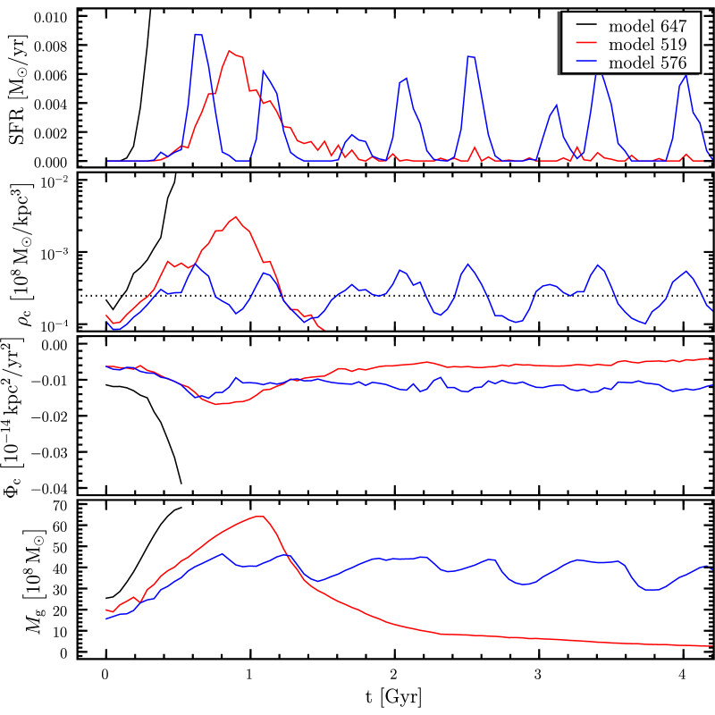
Figure 2: Time evolution of the star formation rate, $\rm{SFR}$, the gas central density, $\rho_{\rm{c}}$, the galaxy central gravitational potential, $\rm{\Phi_{\rm{c}}}$, and the gas mass, $M_{\rm{g}}$ within $3\,\rm{kpc}$. The black line illustrates the case of full gas consumption. The red line stands for the case of an outflow. Finally, the blue line indicates the evolution of a self-regulated model. The dotted black line delimits the star formation threshold density.

Besides this general description common to all simulations, we identify three different major regimes. We refer to them as “full gas consumption”, “outflow” and “self-regulation”. For each of them, Fig. 2 presents the evolution with time of the star formation rate (SFR), the central gas density, the central gravitational potential and the mass of the gas within $3\,\rm{kpc}$ from the galaxy center.

4.1.1 Full gas consumption

In cases where $c_{\star}$ is low for a given $M_{\rm{i}}$, the energy released by the supernova explosions is unable to counterbalance the radiative cooling. As a consequence, the gas keeps on sinking in the galaxy inner regions and reaches very high densities. Stars are formed continuously and at high rate. The model #647 ($c_{\star}=0.05$ and $M_{\rm{i}}=6.6\times 10^{8}\rm{M}_{\odot}$) in Figure 2 provides a clear example of this regime: steep rise in star formation rate and central gas density. The chemical enrichment of the resulting systems is rapid, and their metallicities quickly exceed the highest ones measured in dSphs. These models were not investigated further.

4.1.2 Outflow

Stars can be formed at slightly lower densities by increasing $c_{\star}$ at a given initial mass, or by decreasing the initial mass at fixed $c_{\star}$. This is sufficient to stop the drastic accumulation of gas at the center. Nevertheless, the gas density is still high, and star formation is very efficient. When SNe explode, a huge amount of energy is deposited in the gas, which in turn is expelled from the galaxie’s central regions. In parallel, the central potential increases (it is negative), primarily due to the ejection of the the gas, but also due to the ensuing DM halo expansion. The final consequence is a strong outflow. A large fraction of the total gas mass is ejected beyond a radius of $3\,\rm{kpc}$, chosen to be large enough compared to the stellar extent of the systems. For clarity, we illustrate this regime with M#519 in Fig.2, in which the outflow occurs early in the galaxy evolution: after $\sim 2\,\rm{Gyr}$, there is virtually no gas left.

4.1.3 Self-regulation

Dwarf galaxies are formed in a regime of self-regulation, characterized by successive periods of cooling and feedback. Such intermittent star formation episodes occurring spontaneously in hydrodynamical simulations have been mentioned by Stinson et al. (2007) and Valcke et al. (2008).

M#576 in Fig.2 offers the example of an intermediate mass self-regulated system ($M_{\rm{i}}=4.39\times 10^{8}\,\rm{M_{\odot}}$). As usual, the first contraction of the gas leads to a peak in star formation ($t=0.6\,\rm{Gyr}$). The gas expelled by the supernova feedback is diluted at densities below $\rho_{\rm{sfr}}$, and the star formation stops. As the gas particles cool, they become eligible to star formation again, forming a new burst. Star formation occurs at high frequency in M#576 (periods between $100$ and $200\,\rm{Myr}$). It produces a flat distribution of stellar ages, mimicking a nearly continuous star formation rate (see Fig. 3). We will show later that the corresponding chemical signatures are also very homogeneous.

Contrary to what has been observed by Stinson et al. (2007), the fluctuation of the SF is not strictly periodic. However, we confirm the influence of the total mass $M_{\rm{i}}$ on the duration of the quiescent periods (Valcke et al., 2008). Lower mass systems ($M_{\rm{i}}\lessapprox 3\times 10^{8}\rm{M_{\odot}}$) are generally characterized by star formation episodes separated by longer intervals, up to a few Gyrs. These systems exhibit inhomogeneous stellar populations.

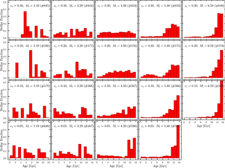
Figure 3: The distributions of stellar ages between $0$ and $14\,\rm{Gyr}$ for a sub-sample of simulations with $f_{\rm{b}}=0.15$ and $r_{\rm{c}}=1$.

4.2 Driving parameters

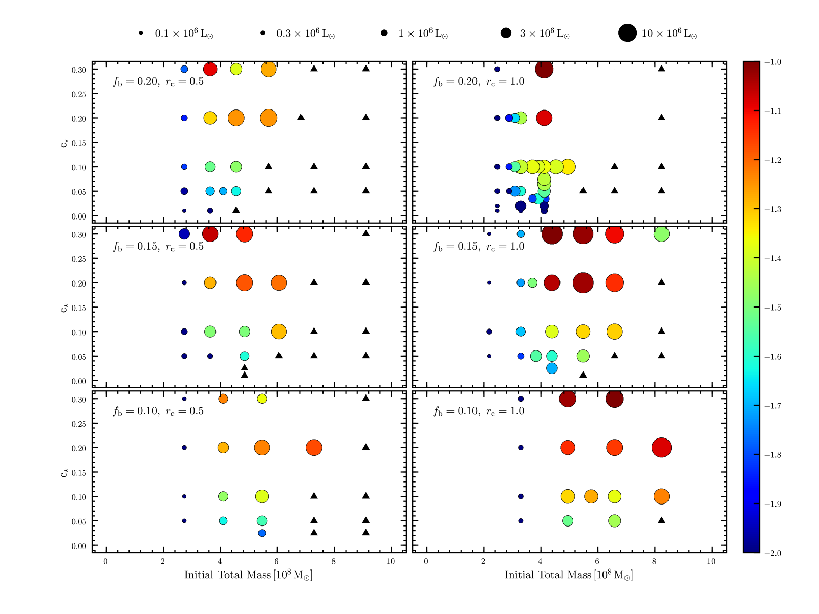
Figure 4: The effect of variation of the model initial parameters. The full sample of simulations is shown. Each circle or triangle stands for one model. The circle size is proportional to the final galaxy luminosity (see the top of the Figure), while colors code the final stellar metallicity (median of the metallicity distribution function), following the scale given at the right hand side of the diagrams. Each panel encompasses simulations of identical baryonic fraction and initial core radius. The black triangles identify cases of full gas consumption.

The description of the different regimes of star formation histories already points out the importance of both the initial total mass, $M_{\rm{i}}$, and the star formation parameter, $c_{\star}$. Figure 3 presents the stellar age histograms for models with $f_{\rm{b}}=0.15$ and $r_{\rm{c}}=1$. From bottom to top, $c_{\star}$ increases by a factor 6. From left to right, $M_{\rm{i}}$ increases by a factor 3. The highest mass systems are characterized by a strong predominance of the old stellar populations. Decreasing the initial total mass extends the period of star formation, passing progressively from a continuous to a discrete distribution of stellar ages. The role of $c_{\star}$ appears secondary, distributing slightly differently the different peaks of star formation (position and strength).

Fig. 4 summarizes the 166  simulations in a diagram of $c_{\star}$ and $M_{\rm{i}}$, for different core radii $r_{\rm{c}}$ and baryonic fractions $f_{\rm{b}}$. Colors code the final galaxy stellar metallicity $\langle\rm{[Fe/H]}\rangle$, computed as the median of the distribution, since it best traces the position of the metallicity peaks in the observations. The size of the circles is proportional to the final stellar luminosity in the $V$-band, $L_{\rm{v}}$. The small black triangles indicate the simulations that lead to full gas consumption and have been stopped. As described earlier, the latters result from a too small $c_{\star}$. It can be avoided, for our purpose, by increasing $c_{\star}$ or decreasing $M_{\rm{i}}$. Self-regulated systems with limited outflow are found for smaller $M_{\rm{i}}$. These tendencies do not dependent on $f_{\rm{b}}$ and $r_{\rm{c}}$, which can only slightly modify the interval of mass in which a particular regime is valid. For a given $c_{\star}$, $\langle\rm{[Fe/H]}\rangle$  increases with $M_{\rm{i}}$ and similarly, for a given $M_{\rm{i}}$, $\langle\rm{[Fe/H]}\rangle$  increases with $c_{\star}$. At very low mass, however, $\langle\rm{[Fe/H]}\rangle$  is only weakly influenced by $c_{\star}$. On the contrary, the larger the mass, the smaller $c_{\star}$ increase is needed to raise $\langle\rm{[Fe/H]}\rangle$.

The left and middle panels of Fig. 5 display the final galaxy stellar metallicity and stellar $V-$luminosity, respectively, as a function of $M_{\rm{i}}$. The Local Group dSphs luminosities (Mateo, 1998; Grebel et al., 2003) and mean metallicities (DART) are indicated with horizontal dotted red lines. The most outstanding result is that changing $M_{\rm{i}}$ by a factor 4 translates to a change in $L_{\rm{v}}$ by a factor 100. $\langle\rm{[Fe/H]}\rangle$  is varied by a factor $\sim$ 3. By comparison, the influence of $c_{\star}$ on the galaxy properties appears small. In any case, increasing $c_{\star}$ will also help increasing both $L_{\rm{v}}$ and $\langle\rm{[Fe/H]}\rangle$. The consequence of varying $M_{\rm{i}}$ is not linear. At low initial mass, a small increase in mass is sufficient to strongly increase $L_{\rm{v}}$ and $\langle\rm{[Fe/H]}\rangle$, while at larger initial mass, the relations saturate and a larger step in mass is necessary. The mass-luminosity and metallicity-luminosity relations will be discussed in the next section.

The right panel of Fig. 5 presents the relation between the galaxy’s mean stellar age and $M_{\rm{i}}$. The influence of $c_{\star}$ looks more linear than previously on $L_{\rm{v}}$ and $\langle\rm{[Fe/H]}\rangle$. As a matter of fact, we have seen in Fig. 3 that it plays a role in the stellar age distribution. At a given initial mass, $c_{\star}$ determines the length of the star formation periods as well as the interval between them.

As a conclusion, the above analyses stress the primordial impact of the initial total mass of the systems. Moreover, one can clearly identify the range of possible $M_{\rm{i}}$ leading to the formation of the Local Group dSphs as we observed them today. This range is narrow, e.g, a factor 2 centered on $M_{\rm{i}}\geq 5\times 10^{8}\rm{M_{\odot}}$.

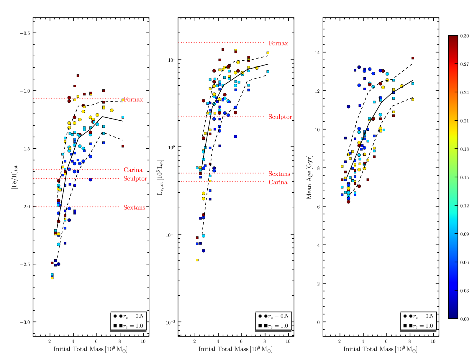
Figure 5: The metallicity, $\langle\rm{[Fe/H]}\rangle$, luminosity in $V$-band, $L_{\rm{v}}$, and stellar mean age as a function of the galaxy’s total initial mass, after $14\,\rm{Gyr}$ of evolution. The circles and squares correspond to $r_{\rm{c}}=0.5$ and $r_{\rm{c}}=1$, respectively. The colors encode $c_{\star}$ following the scale at the right-most panel of the figure. The positions of our four targeted dSphs are indicated with red dotted lines. Plain line indicate the mean values, while dashed ones indicate the one sigma deviation.

5 Global relations

dSph galaxies follow luminosity-mass and luminosity-metallicity relations that are considered as cornerstones to understanding their formation and evolution (Mateo, 1998; Wilkinson et al., 2006; Gilmore et al., 2007; Strigari et al., 2008; Geha et al., 2008; Kirby et al., 2008).

In the following discussion, we calculate all physical quantities (luminosities, masses, abundances) within the radius $R_{\rm{L}}$ defined as the radius containing 90% of a galaxy’s total luminosity. This choice is guided by the wish to reproduce as closely as possible the observational conditions under which these quantities are measured. The classical dSphs (as opposed to newly discovered faint ones) surrounding the Milky Way have tidal radii in the range $\sim$ $0.5\,\rm{kpc}$ to $3\,\rm{kpc}$ (Irwin & Hatzidimitriou, 1995). Fixing a constant small aperture for all dSphs would underestimate both light and mass of the largest systems. Since dark matter does not necessarily follow light, this would also bias the results. The observational estimates of the dSph total masses are based on stellar velocity dispersions measured at galactocentric radii as large as possible, thereby directly linked to the limits of the visible matter. Although the farthest measurements do not always reach the galaxies’ tidal radii, their location is determined by severe drops in stellar density, ensuring that the bulk of the galaxies’ light is enclosed. Consequently, we compare our models to the masses derived at the outermost velocity dispersion profile point (e.g, Walker et al., 2007; Battaglia et al., 2008a; Kleyna et al., 2004). Ursa Minor is the only exception to this rule. Its mass has been derived from its central velocity dispersion (Mateo, 1998).

Figures  6 and 7 display the relations of the galaxies’ mass-to-light ratios $M/L_{\rm{v}}$ and the median of the stellar metallicity distributions $\langle\rm{[Fe/H]}\rangle$, together with the total luminosity of the model galaxies. The observations are represented in red, with squares for the Milky Way satellites and crosses for the others. In general, the values of $\langle\rm{[Fe/H]}\rangle$ are taken from Mateo (1998) when available or from Grebel et al. (2003) otherwise. The mean metallicities of Carina, Fornax, Sculptor, and Sextans are calculated from their metallicity distributions (Helmi et al., 2006; Battaglia et al., 2008a, 2006).The mean metallicity of Leo II is derived from the metallicity distribution of Bosler et al. (2007). The luminosities are taken from Grebel et al. (2003), with the exception of Draco (Martin et al., 2008). The masses of Carina, Fornax, Draco, Leo I and Leo II are computed by Walker et al. (2007) inside $r_{\rm{max}}$. The mass of Sextans corresponds to the upper limit of Kleyna et al. (2004), while the mass of Ursa Minor comes from Mateo (1998). Sculptor’s $M/L_{\rm{v}}$ is taken from Battaglia et al. (2008a).

Both $M/L_{\rm{v}}$ and $\langle\rm{[Fe/H]}\rangle$  show very clear log-linear relations with $L_{\rm{v}}$:

$$\log_{10}\left(M/L\right)=-0.79\log_{10}\left(L_{\rm{v}}/L_{\odot}\right)+1.85,$$ (17)

and

$$\langle\rm{[Fe/H]}\rangle=0.68\log_{10}\left(L_{\rm{v}}/L_{\odot}\right)-1.8.$$ (18)

Despite differences in $c_{\star}$, $r_{\rm{c}}$ and $f_{\rm{b}}$, all simulations nicely reproduce the observations, with a reasonably small scatter. This stresses once more that a dSph galaxy’s total initial mass drives most of its evolution.

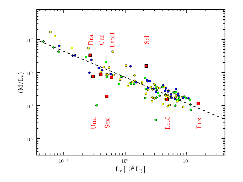
Figure 6: The galaxies’ mass-to-light ratios, $M/L_{\rm{v}}$, versus their total luminosities $L_{\rm{v}}$ in the $V$-band. Each circle stands for a model. Colors encode the three different initial baryonic fractions that we have considered, $f_{\rm{b}}=0.2$ (yellow), $f_{\rm{b}}=0.15$ (green) and $f_{\rm{b}}=0.1$ (blue). The red squares represent the Milky Way brightest dSphs. The best fit to our data (Eq. 17) is indicated by the dashed line.

Figure 7: The median of the galaxies’ metallicity distributions, $\langle\rm{[Fe/H]}\rangle$, as a function of their luminosities $L_{\rm{v}}$. Each circle stands for a model. Colors encode the three different baryonic fractions that we have considered, $f_{\rm{b}}=0.2$ (yellow), $f_{\rm{b}}=0.15$ (green) and $f_{\rm{b}}=0.1$ (blue). The best fit to our data (Eq. 17) is indicated by the dashed line. The red squares represent the Milky Way’s brightest dSph satellites, the red crosses represent the M31’s ones.

To allow deeper insight into the building up of the $M/L_{\rm{v}}-L_{\rm{v}}$ relation, Fig. 8 distinguishes between dark matter (DM), stars and gas. Colors encode the three different initial baryonic fractions that we have considered, $f_{\rm{b}}=0.2$ (yellow), $f_{\rm{b}}=0.15$ (green) and $f_{\rm{b}}=0.1$ (blue).

Figure 8: The relation between galaxy mass and $V$-band luminosity for the the dark matter, the stars and the gas. The lower panel displays the gas over stars mass ratio. Colors encode the three different baryonic fractions that we have considered, $f_{\rm{b}}=0.2$ (yellow), $f_{\rm{b}}=0.15$ (green) and $f_{\rm{b}}=0.1$ (blue).

Very naturally, stellar mass scales with the luminosity. At fixed luminosity, the dispersion in stellar mass is of the order of $5\times 10^{6}$M_⊙. In fact, a more appropriate way to look at this panel is to consider the dispersion in luminosity at fixed stellar mass, since the dispersion in luminosity is a direct consequence of various distributions in stellar ages and metallicities. This dispersion, of the order of $10^{6}\,\rm{L_{\odot}}$. It increases slightly for larger masses, for which star formation can last longer, inducing a larger number of possible age/metallicity combinations.

As already discussed in Fig. 5, whilst $L_{\rm{v}}$ spans nearly 3 orders of magnitude, the mass of dark matter varies little. This variation is much less than one order of magnitude inside $R_{\rm{L}}$ and is mostly due to the dispersion among the models. A common mass scale (inside $R_{\rm{L}}$), around $1-5\times 10^{7}\,\rm{M_{\odot}}$, for the dSph total masses seems also favored by the observations, although an exact value for this limit is difficult to ascertain, given the large uncertainties of the mass estimates in general (Mateo, 1998; Gilmore et al., 2007; Strigari et al., 2008).

Interestingly, one can now witness the effect of varying the initial baryonic fraction. Galaxies with $L_{\rm{v}}<3\times 10^{6}\,\rm{L_{\odot}}$ exhibit identical DM halo masses, whatever $f_{\rm{b}}$, while for larger luminosities, the models of lowest $f_{\rm{b}}$ require larger halo masses in order to generate a similar quantity of stars. For $f_{\rm{b}}=0.20$, the DM halo mass is constant over the whole luminosity range. This demonstrates that while dark matter plays a crucial role in confining the gas, the amount of the latter is also important for the most massive dSphs: it must reach a critical amount to enable their formation.

The third panel of Fig. 8 displays the mass of residual gas after $14\,\rm{Gyr}$. It constitutes a very small fraction of the total mass, and is therefore undetectable at the level of the scaling relations. Quite interestingly, its amount is of the order of the HI mass observed in dwarf irregular galaxies (dIs) (Grebel et al., 2003) and is weakly dependent on the total luminosity. Nevertheless, there is a non-intuitive tendency for the most luminous galaxies ($>5\times 10^{6}\,\rm{L_{\odot}}$) to exhibit less gas than the rest of the systems on the sequence. However, the most massive galaxies succeed in retaining most of their gas despite the supernova explosions. Less than 60% of their gas is ejected, while this fraction lies between 70% and 90% for less massive systems, in agreement with the results of Valcke et al. (2008). However, the star formation efficiency is also higher in more massive galaxies. As a result, the gas consumption counterbalances the presence of the large gas reservoir. We will come back to this in Section 7.

Since the gas mass is very much constant at around $10^{7}\,\rm{M_{\odot}}$, the smallest galaxies have proportionally more gas than the massive ones (see bottom panel of Fig. 8). Below $3\times 10^{6}\,\rm{L_{\odot}}$, galaxies have more gas left than they have formed stars. Their gas to stellar mass ratios reach 100 at the faint end of the dSph model sequence. Meanwhile, stars dominate over gas by a factor 5 for the most luminous galaxies.

As a conclusion, the lessons to be taken from Fig. 8 are twofold: i) all dSphs are clearly dominated by dark matter. The lower the mass of the system, the lower the final baryonic fraction. ii) all model galaxies present an excess of gas at the end of their evolution, as has been found in similar studies (Marcolini et al., 2006, 2008; Stinson et al., 2007; Valcke et al., 2008). As demonstrated earlier, dSphs cannot originate from smaller amounts of gas (for a given final luminosity, metallicity and age). It is necessary to initiate the star formation in the observed proportions. However, it is not yet clear how much of this gas must be kept in the subsequent phases of the galaxy evolution. It is clear that the excess of gas, observed in models in isolation, must in reality have been stripped some time during the galaxy evolution.

The quantity of gas falls in the range of HI mass observed in dIs, always found further away than dSphs from their parent galaxies, thereby bringing another piece of evidence for the role that interactions might play in its removal. It might also be achieved in a hierarchical formation framework, for which the gravitational potentials are initially weaker.

As we have just shown, the global scaling relations are reproduced by our model with impressive ease. In turn, this conveys the idea that the global scaling relations do not form a very precise set of constraints. They do not reflect the diversity in star formation histories that we have illustrated. In order to understand the individual histories of the Local Group dSphs, one definitely needs to go one step further and consider their chemical abundance patterns, as well as the information that color-magnitude diagrams provide on the stellar age distributions.

6 Generic models

We will now select and discuss a series of generic models reproducing the properties of four Milky Way dwarf spheroidals, Carina, Fornax, Sculptor and Sextans. The choice of these models is based on four observational constraints:

• The dSph total luminosity, which scales with the total amount of matter involved in the galaxy star formation history.

• The metallicity distribution which traces the star formation efficiency.

• The chemical abundance patterns, in particular that of the $\alpha$-elements, that determines the length and efficiency of the star formation period together with its homogeneity. We use magnesium for the $\alpha$-elements. [Fe/H] and [Mg/H] are derived from high resolution spectroscopy in the central regions of the galaxies (Hill et al in preparation; Letarte et al. in preparation; Venn & Hill, 2005; Letarte et al., 2007; Shetrone et al., 2003; Koch et al., 2008).

• The stellar age distributions. They complement the above constraints with information on possible series of bursts (Smecker-Hane et al., 1996; Hurley-Keller et al., 1998; Coleman & de Jong, 2008).

Table 1 lists the initial parameters of our generic models. Table 2 lists their final properties, namely the stellar luminosity in the $V$-band, $L_{\rm{v}}$, the mass-to-light ratio, $M/L_{\rm{V}}$, the gas mass, $M_{\rm{gas}}$, the median metallicity, $\langle\rm{[Fe/H]}\rangle$, the fraction of stars with [Fe/H] lower than $-3$ and, finally, the stellar age distribution divided in 3 bins: younger than $4\,\rm{Gyr}$, between $4$ and $8\,\rm{Gyr}$ and older than $8\,\rm{Gyr}$.

Fig. 11, 12 and 13 display the stellar metallicity distribution, the [Mg/Fe] vs [Fe/H] diagrams and the stellar age histograms, respectively, after $14\,\rm{Gyr}$ of evolution. Fig. 14 shows the stellar age-metallicity relations.

We do not try to match exactly all properties of our target dSphs. Instead, we select the four most satisfying models in our sample of 166. More specifically, we allow a freedom of a factor 2 in luminosity and a shift of a few tenths of dex in peak [Fe/H]. It is beyond doubt that we could fine-tune $M_{\rm{i}}$, $c_{\star}$, $r_{\rm{c}}$ and $f_{\rm{b}}$ to exactly reproduce the observations. However, this is beyond our scope, which remains to test the hypothesis of a formation framework common to all dSphs. The dependence of the results on the model parameters is illustrated in Fig. 9 and 10. We selected 6 models at low ($L_{\rm{v}}\cong 0.5\times 10^{6}\,\rm{M_{\odot}}$) and high ($L_{\rm{v}}\cong 3.7\times 10^{6}\,\rm{M_{\odot}}$) luminosities. The baryonic fraction is fixed each time, and only $c_{\star}$ and $M_{\rm{i}}$ vary. One sees that around a given fixed core of observed characteristics (e.g, luminosity, metallicity), we could run the models on a finer grid of parameters in order to match the galaxy properties in all details. This means, for example, to exactly reflect the stellar age distribution, or the spread in abundance ratios.

Figure 9: The variation in [Mg/Fe] vs [Fe/H], [Fe/H] distribution and stellar age distribution for 3 models of similar luminosities ($L_{\rm{v}}\cong 0.5\times 10^{6}\,\rm{M_{\odot}}$) and identical initial baryonic fraction ($f_{\rm{b}}=0.15$). The stellar fraction is defined as the number of stars in each bin divided by the total number of stars.

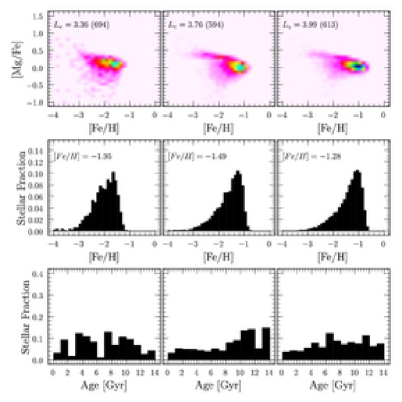
Figure 10: Same as Fig. 9 but for a brighter set of model galaxies ($L_{\rm{v}}\cong 3.7\times 10^{6}\,\rm{M_{\odot}}$)

6.1 Global evolution

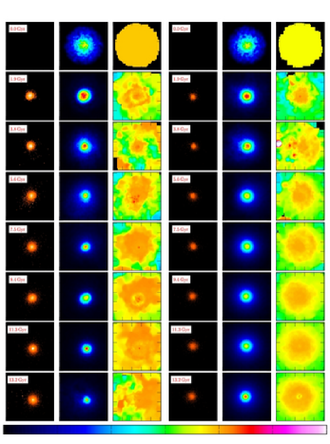
Figure 16: Stellar, gas and temperature evolution of the models #575 (Fornax) and #630 (Sculptor) as a function of time. Each model is illustrated with three columns: The first column presents the stellar surface brightness in log scale, between $0$ and $0.4\,\rm{L_{\odot}}/kpc^{2}$, the second one, the gas surface density in log scale, between $0$ and $1.5\times 10^{7}\,\rm{M_{\odot}}/kpc^{2}$, the third one gives the log of the gas temperature, between $10^{2}$ and $10^{5}\,\rm{K}$. While intervals are different for the gas surface density and temperature, the principle of the color coding remains similar: white-red colors for high values and blue-black colors for low values, as indicated by the horizontal bar at the bottom of the figure. The size of each panel is $20\times 20\,\rm{kpc}$.

Fig. 16 and 17 show the stellar surface density, the gas surface density and the gas temperature between $0$ and $14\,\rm{Gyr}$ for our four selected generic models. Not only do these reproduce the properties of Carina, Fornax, Sculptor and Sextans individually, but they also depict the full spectrum of evolutions seen in our models. The size of each panel is $20\times 20\,\rm{kpc}$.

All gas particles initially share the same temperatures, corresponding to the galaxy virial temperature, as given by Eq. 16. As soon as the simulations start, the gas looses energy by radiative cooling. Consequently, the gas density increases in the galaxy central regions. Red areas in the gas density maps identify densities larger than $\rho_{\rm{sfr}}$, i.e., they mark regions where gas particles may be eligible for star formation. When this is indeed the case, the newly formed stars are traced by their high brightness in the stellar density maps.

The SN explosions induce temperature inhomogeneities. Indeed, the heated central gas expands and generates a wave propagating outwards. If the SN feedback dominates the cooling, the gas is diluted and the red color vanishes from the center of the gas density maps: star formation is quenched. Such quiescent periods are characterized by a nearly constant and homogeneous central temperature $\sim 10^{4}\,\rm{K}$, the temperature at which the radiative cooling counterbalances the adiabatic heating. When gas has sufficiently cooled, it can condense again, and star formation is induced again. These periods of star formation and quiescence alternate at low or high frequency, depending on the mass of the galaxy. For low-mass systems, the cooling time is of the order of several Gyrs, it is much shorter for more massive ones. We will now see how each of these cases translate into dSph stellar population properties.

Figure 11: The stellar [Fe/H] distributions of the four generic models reproducing Carina, Sextans, Sculptor and Fornax. The model outputs are shown in black and the observations with red dashed lines. The stellar fraction is defined as the number of stars in each bin divided by the total number of stars.

Figure 12: The stellar [Mg/Fe] vs [Fe/H] diagrams for the four generic models reproducing Carina, Sextans, Sculptor and Fornax. The observations are sketched with black dots. Their error bars are shown. Colors encode the fraction of stars as indicated by the bar at the top.

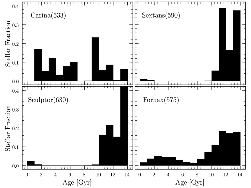
Figure 13: The stellar age distributions of the four generic models. The stellar fraction is defined as the number of stars in each bin divided by the total number of stars.

Figure 14: The age-metallicity relations of the four generic models. Each dot corresponds to a stellar particle.

6.2 Sextans

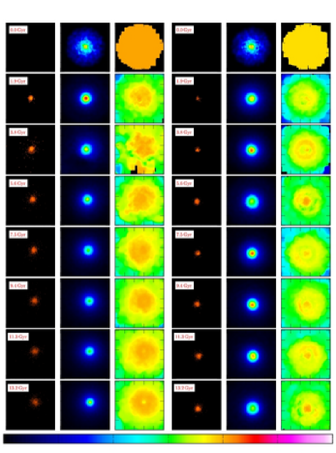
Figure 17: Same as Fig. 16 but for the models #590 (Sextans) and #533 (Carina).

The stellar population of Sextans is dominated by stars older than $10\,\rm{Gyr}$ (Lee et al., 2003). With its mean metallicity $\langle\rm{[Fe/H]}\rangle=-2.05$ and a $V$-band total luminosity of $0.5\times 10^{6}\,\rm{L_{\odot}}$, it falls exactly on our luminosity-metallicity relation (Fig. 7), and its properties are reproduced by the model #590 ($L=0.53\times 10^{6}\,\rm{L_{\odot}}$, $\langle\rm{[Fe/H]}\rangle=-2.02$ ) that experiences an outflow. Sextans’ evolution is dominated by an early period of star formation lasting about $3\,\rm{Gyr}$. The gas surface density map of Fig. 17 shows the dense central region at the origin of the star formation burst ($t=1.9\,\rm{Gyr}$). At that time, a small but bright stellar system is already formed. After this period, the gas is expelled and diluted. No star can form until the last $\rm{Gyr}$, when the gas has sufficiently cooled down to fulfill the star formation criteria. This last episode of star formation is an artifact of the gas retained by our model, as discussed in Section 5. It is however negligible compared to the bulk of the population and does not influence Sextans’ properties.

Fig. 12 shows that the bulk of Sextans model stars are located at [Mg/Fe] $\cong 0.3$, with however a noticeable dispersion at lower values. The dispersion originates from the uneven intensities of the star formation peaks. They create regions with diverse levels of chemical enrichment. When the intensity of star formation rises again after a period of semi-quiescence, the ejecta of new SNe II are mixed with material of low $\alpha$-element abundance. Refinement of the model would require a larger sample of observed stars at high resolution, particularly to estimate the statistical significance of the dispersion in [Mg/Fe].

6.3 Carina

Carina seems to have experienced a complex evolution characterized by episodic bursts of star formation, with at least three major episodes at around $15$, $7$ and $3\,\rm{Gyr}$ , and a period of quiescence between $7$ and $3\,\rm{Gyr}$ (Smecker-Hane et al., 1996; Hurley-Keller et al., 1998). Our set of simulations reveal that episodic bursts of star formation are intrinsic features of the self-regulated low initial masses systems ($M_{\rm{i}}\lessapprox 3\times 10^{8}\,\rm{M_{\odot}}$, see Fig. 3). Shortly after a star formation episode, supernovae explode, gas is heated and expands. Because its density is low, its cooling time is of the order of several Gyrs. This series of well spaced-out SF peaks translate into dispersion in [Mg/Fe] at fixed [Fe/H]. This spread is more accentuated than for Sextans, due to the extended star formation and the longer intervals between bursts.

Fig. 7 shows that Carina, with $\langle\rm{[Fe/H]}\rangle=-1.82$ and $L_{\rm{v}}=0.72\times 10^{6}\,\rm{M_{\odot}}$, falls above the relation [Fe/H]-$L_{\rm{v}}$ defined by our models. As already mentioned, we give priority to constraints provided by the spectroscopic data, and allow some flexibility in $L_{\rm{v}}$. Under these conditions, model #533 ($M_{\rm{i}}=2.7\times 10^{8}\,\rm{M_{\odot}}$) provides a very reasonable fit to Carina’s properties. The three major SF episodes are reproduced: 45% of the stars have ages between $9$ and $15\,\rm{Gyr}$, 29% have $4$ to $8\,\rm{Gyr}$ and 22% are younger than $3\,\rm{Gyr}$. Whilst Carina is somewhat less luminous than Sextans, its mean metallicity is higher. This is due to a lower initial mass, locking less matter in stars, but a longer period of star formation, obtained by a slightly higher star formation parameter, which avoids outflows.

6.4 Sculptor

The Sculptor dSph has formed stars early, over a period of a few Gyrs. No significant intermediate age population has been found, hence excluding star formation within the last $\sim 5\,\rm{Gyr}$. The evidence for low $\alpha$-element enhancement agrees with an extended star formation and self-enrichment over a period of at least $2\,\rm{Gyr}$ (e.g. Babusiaux et al., 2005; Shetrone et al., 2003; Tolstoy et al., 2003).

Sculptor’s properties are well reproduced by model #630 ($L=2.86\times 10^{6}\,\rm{L_{\odot}}$, $\langle\rm{[Fe/H]}\rangle=-1.82$). The outstanding feature of Sculptor, as compared to the two previous dSph, is the small dispersion in the [Mg/Fe] vs [Fe/H] diagram (Fig. 12). This is guaranteed by a strong initial star formation, followed by subsequent episodes of lower, but smoothly decreasing intensities, ensuring the chemical homogeneity of the interstellar medium.

6.5 Fornax

Fornax is obviously the most challenging case of dSphs. It is the most luminous of all ($15.5\times 10^{6}\,\rm{L_{\odot}}$), it is metal-rich ($\langle\rm{[Fe/H]}\rangle=-1.07$) and has experienced multiple periods of star formation. Indeed, in addition to very old stars, Fornax reveals a dominant intermediate-age population, as well as stars of $\sim 3-4\,\rm{Gyr}$ (Coleman & de Jong, 2008).

Fornax is nicely reproduced by the self-regulated model #575. Stars are formed in a high frequency series of short bursts, lasting between $200$ and $500\,\rm{Myr}$. The amplitude of these bursts progressively decreases with time, until $\sim 7\,\rm{Gyr}$. Thereafter, part of the gas that had been expelled by previous SN explosions, has sufficiently cooled to restore star formation, at $\sim 3\,\rm{Gyr}$, similar to what is observed. The succession of the short bursts of similar intensities mimics a continuous star formation and leads to an efficient and homogeneous chemical enrichment ($\langle\rm{[Fe/H]}\rangle=-1.03$).

We reach a luminosity $L=12.6\times 10^{6}\,\rm{L_{\odot}}$, slightly below the observation of Fornax. However, just as in the case of Carina, the exact value of the $V$-band luminosity is very sensitive to the exact amount of stars formed in the last Gyrs and may easily vary. Stars form up to the end of the simulation. This is consistent with the observational evidence of a small number of $100\,\rm{Myr}$ stars (Coleman & de Jong, 2008).

Figure 14 show the stellar age-metallicity relations of our four generic models. In all cases, we are far from a one to one correspondence between age and metallicity, although below [Fe/H]=-2.5 (but more safely below [Fe/H]=$-3$), stars are generally older than 10 Gyr. The dispersion in metallicity is in the range 0.5 to 1 dex at ages younger than 10 Gyr.

Figure 15: The [Mg/Fe] vs [Fe/H] diagram, the stellar [Fe/H] distribution, the age-metallicity relation and the global stellar age distribution of the model #587, compared to the observations of Leo II

dSph	#	$r_{\rm{c}}$	$f_{\rm{b}}$	$c_{\star}$	$\rho_{\rm{c,tot}}$	$M_{\rm{tot}}$
		$[\rm{kpc}]$			$[10^{8}\,\rm{M_{\odot}/kpc^{3}}]$	$[10^{8}\,\rm{M_{\odot}}]$
Carina	$533$	0.5	0.20	0.100	1.20e-03	2.73
Leo II	$587$	1.0	0.15	0.050	4.00e-04	3.29
Sextans	$590$	0.5	0.15	0.050	1.60e-03	3.64
Sculptor	$630$	1.0	0.20	0.035	5.00e-04	4.12
Fornax	$575$	1.0	0.15	0.200	6.66e-04	5.48

Table 1: Initial parameters of the five generic models.

dSph	#	$L_{\rm{v}}$	$M/L_{\rm{V}}$	$M_{\rm{gas}}$	$\langle\rm{[Fe/H]}\rangle$	$\rm{[Fe/H]}<-3.0$	$\leq 4\,\rm{Gyr}$	$[4,8]\,\rm{Gyr}$	$\geq 8\,\rm{Gyr}$
		$[10^{6}\,\rm{L_{\odot}}]$		$[10^{8}\,\rm{M_{\odot}}]$	dex	%	%	%	%
Carina	$533$	0.72	231	0.28	-1.82	2.9	26.1	29.3	44.6
Leo II	$587$	0.97	219	0.33	-1.82	2.9	24.4	26.4	49.2
Sextans	$590$	0.53	390	0.17	-2.02	5.2	1.7	0.0	98.3
Sculptor	$630$	2.86	83	0.32	-1.82	5.6	3.6	0.0	96.4
Fornax	$575$	12.76	27	0.12	-1.03	1.2	14.4	10.6	75.0

Table 2: The final properties of the five selected generic models. ($L_{\rm{v}}$) : stellar luminosity in $V$-band, ($M/L_{\rm{V}}$) : mass-to-light ratio, ($M_{\rm{gas}}$) : gas mass, ($\langle\rm{[Fe/H]}\rangle$) : median of the metallicity distribution function, ($\rm{[Fe/H]}<-3.0$) : fraction of stars having a metallicity lower than $-3$, ($\leq 4\,\rm{Gyr}$) : fraction of stars younger than $4\,\rm{Gyr}$, ($[4,8]\,\rm{Gyr}$) : fraction of stars having ages between $4$ and $8\,\rm{Gyr}$, ($\geq 8\,\rm{Gyr}$) : fraction of stars older than $8\,\rm{Gyr}$.

6.6 Leo II

While writing up our results, the abundance ratios in a sample of 24 stars in Leo II have been published (Shetrone et al., 2009). We keep Leo II separated from the other individual case analyses, since its abundance ratios have been obtained from lower resolution spectra and therefore have larger uncertainties.

Fig. 15 illustrates how model #587 can reproduce the star formation history of Leo II. The observed metallicity distribution, derived from $\sim 100$ stars, is taken from Bosler et al. (2007), and [Mg/Fe] from (Shetrone et al., 2009). Leo II has a luminosity similar to that of Sextans, but unlike Sextans, Leo II sustained a low but constant star formation rate, leading to an important intermediate age stellar population (Mighell & Rich, 1996; Koch et al., 2007). The reason for a continuous (low) star formation in Leo II’s model is found in the slightly smaller initial total mass for the same star formation parameter as Sextans; it prevents the gas outflow. Carina and Leo II have about the same mean metallicities. They probably have probably experienced a very similar evolution, as indeed seen in Table 2 for their mean properties. However, the two galaxies indeed differ: i) by the periods of quiescence which are longer in Carina, and ii) by the extent of the star formation peaks, which are between 2 to 3 times longer in Leo II, at intermediate ages. Model #587 produced a higher final luminosity than observed, due to the presence of residual gas and therefore recent star formation, as in all the models. It is important to recall that we do not aim at reproducing Leo II properties in fine details, but instead check whether its main features exist in the series of models we ran. In this respect, model #587 demonstrates that a low level of rather continuous star formation is indeed achievable.

The extension of the sample of stars with spectroscopic data allowing measurements of abundance ratios would greatly help the precise identification of Leo II model. This is particularly true at [Fe/H] $>-1.6$ which would confirm or not the apparent plateau in [Mg/Fe]. Even more decisive and more general, one needs to observationally confirm or disprove the dispersion in [Mg/Fe] at low and moderate metallicities in low mass dSphs, as it signals the discrete nature of star formation as advocated by contemporary models.

Table 1 gives the fraction of very-metal poor ([Fe/H]$<-3$) stellar particles in the generic models. The general trend of our series of 166  models is that the more extended the star formation period, the smaller this fraction. This is clearly illustrated by the models of Carina and Fornax, as compared to those of Sextans and Fornax. Although the tail of very metal-poor stars is small (from$\sim$ 1 to 6%), it is still larger than suggested by the observations to date (Helmi et al., 2006). In order to properly address this particular issue, one needs i) to investigate the impact of more sophisticated IMFs, such as the one of Kroupa et al. (1993), for which the number of low-mass stars is smaller than for a Salpeter IMF, and ii) to introduce the peculiar features of star formation at zero metallicity. The conditions of transition between population III and population II star formation depends on the galaxy halo masses, and so is the galaxy metallicity floor (Wise & Abel, 2008). This opens a independent new field of investigation. For the time being, we check our model predictions against population II properties. Interestingly, the outflows generated by these very first generation of stars offers an alternative solution to get rid of the final excess of gas.

6.7 Mass profiles and velocity dispersions

Although our primary goal is not to match the morphology of the dSphs, we have considered the shape of the final modeled dSph profiles within $R_{\rm{L}}$. Fig. 18 displays the mass density profiles of the stellar and dark components for our four main targets. Each model is successfully fitted by a Plummer model, revealing a flat inner profile, in agreement with the observations. The ratio between the stellar and dark core radii $r_{c}^{\rm{stars}}/r_{c}^{\rm{halo}}$ ranges between $0.2$ and $0.5$, indicating a spatial segregation of the stars relative to the dark halo, as discussed in (Peñarrubia et al., 2008). Additionally, the line-of-sight stellar velocity dispersion profiles are flat in the enclosed within the core radii, with $6$ to $10\,\rm{km/s}$, corresponding to the least and the most massive dSph, respectively, hence well within the observed range (Walker et al., 2006a; Muñoz et al., 2006; Battaglia et al., 2008a; Walker et al., 2006b).

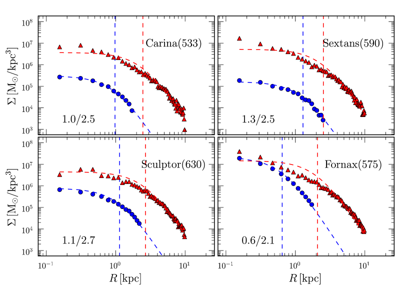
Figure 18: The stars (blue circles) and dark halo (red triangles) density profiles for the four generic models. Each profile is fitted by a Plummer model. The positions of the core radii are indicated by the dashed lines. Their values are given in the left bottom corner of each panel.

7 Discussion

We have shown that the total initial mass $M_{\rm{i}}$ and $c_{\star}$ are the two driving parameters for the evolution of dSphs. Our models which describe galaxies in isolation, i.e., not yet taking into account interactions or accretions that inevitably occur in a $\Lambda$CDM Universe, already lead to the observed variety of star formation histories. Decreasing the initial total mass of the galaxies separates the periods of star formation.

The marked differences found between high- and low mass systems is a key point in understanding the formation of dSphs. In order to illustrate our findings, we now focus on cooling time and gas temperature. The top panel of Fig. 19 displays the galaxy’s virial temperature as a function of its initial mass (Eq. 16).

The green horizontal band indicates the temperature at which the cooling time of the gas is equal to $100\,\rm{Myr}$, for two threshold densities, $\rho_{\rm{sfr}}$ and $10^{-3}\,\rho_{\rm{sfr}}$ that are representative of the range in gas density observed in the course of our simulations. The value of $100\,\rm{Myr}$ is chosen to be short compared to the galaxy lifetimes. The lower border of the green band corresponds to $\rho_{\rm{sfr}}$ while the upper ones correspond to $10^{-3}\,\rho_{\rm{sfr}}$. The intersection between the green band and the curves corresponds to a total mass ranging between $3$ and $4\times 10^{8}\,\rm{M_{\odot}}$, delimiting two regimes distinguished by long and short cooling times, as can be measured in the bottom panel of Fig. 19. The cooling times of $\rho_{\rm{sfr}}$ and $10^{-3}\,\rho_{\rm{sfr}}$ as a function of the galaxy initial masses are shown in solid and dashed lines, respectively, in the bottom panel of the figure. They are calculated by taking the virial temperature of the corresponding galaxy mass. The gas contained in galaxies of total masses larger than $4\times 10^{8}\,\rm{M_{\odot}}$, with corresponding virial temperatures larger than $10^{4}\,\rm{K}$ is characterized by a short cooling time ($\tau<$100 Myr) at all densities. This short cooling time is due to the strong radiative cooling induced by the recombination of hydrogen above $10^{4}\,\rm{K}$. A galaxy which is in this cooling regime will see its gas loosing a huge amount of energy, sinking in its central regions and inducing star formation. This is precisely what happens in the model #575 where stars are continuously formed, generating a metal-rich Fornax-like system. By decreasing the total mass from $4$ to $3\times 10^{8}\,\rm{M_{\odot}}$, the virial temperature falls below the peak of hydrogen ionization. As a consequence, the cooling function drops and the cooling time is increased by nearly three orders of magnitude. Below $3\times 10^{8}\,\rm{M_{\odot}}$, the cooling time is long, since the loss of energy by radiative cooling is strongly diminished. In this regime, star formation can only occur in episodic bursts, separated by periods corresponding to the mean cooling time. Carina gives a clear example of such a case. For even lower mass systems ($M_{\rm{tot}}<10^{8}\rm{M_{\odot}}$), the cooling time is longer than $10\,\rm{Gyr}$, and therefore no stars are expected to form.

From our simulations, a total mass of $\sim 4\times 10^{8}\,\rm{M_{\odot}}$ leads to a luminosity of $\sim 3\times\,10^{6}\,\rm{L_{\odot}}$. Not surprisingly, this luminosity corresponds to the critical one found in Section 5, below which the galaxies have more gas left than they have formed stars. The sharp cutoff of the cooling function below $4\times 10^{8}\,\rm{M_{\odot}}$ explains very nicely why a small decrease in mass induces a large drop in luminosity, seen in the middle panel of Fig. 5. A direct consequence is the constancy of galaxy masses within $R_{\rm{L}}$ ($\sim 1-5\times 10^{7}\,\rm{M_{\odot}}$) over the wide range of dSph luminosities, as discussed in Section 5 (Fig. 8) and suggested by Mateo (1998), Gilmore et al. (2007) and Strigari et al. (2008).

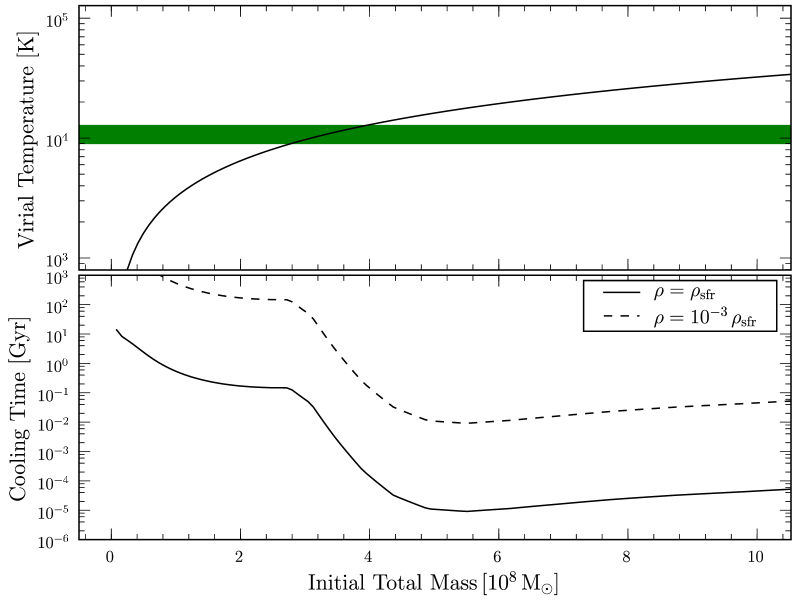
Figure 19: Top: The Virial temperature as a function of the total initial mass computed from Eq. 16, with $r_{\rm{c}}=1\,\rm{kpc}$. The lower border of the green band gives the Virial temperature of gas with density equal to $\rho_{\rm{sfr}}$. The upper border indicates the Virial temperature of gas with density equal to $10^{-3}\,\rho_{\rm{sfr}}$. The cooling time is of the order of $0.1\,\rm{Gyr}$. Bottom: Cooling time of the gas as a function of the total mass, assuming a Virial temperature given by Eq. 16. The case of a gas density equal to $\rho_{\rm{sfr}}$ is shown by the solid line, while the density of $10^{-3}\,\rho_{\rm{sfr}}$ is shown by the dashed line.

The next step in simulating the formation and evolution of dSph galaxies is to study the impact of external processes resulting from a $\Lambda$CDM complex environment, like tidal mass stripping, ram stripping, dark matter and gas accretion, as well as reionization and self-shielding. Peñarrubia et al. (2008) show that tidal mass stripping strongly depends on the spatial distribution of stars relative to the dark halo extent. If stars are very concentrated in large halos, dSphs will be more resilient to tidal disruption. Dwarf spheroidal galaxies may need to loose nearly $90\%$ of their mass before their star formation and therefore chemical evolution start to be affected. Mayer et al. (2006) tackle all the above listed questions and show how their mechanisms can be interlaced. As an example, in their models gravitational tides help ram pressure stripping by diminishing the overall potential of the dwarf, but tides induce bar formation making subsequent stripping more difficult. Reionization prevent star formation, but self-shielding helps cooling. Clearly, understanding the impact of these physical processes on our specific modeling requires dedicated simulations.

8 Summary

We have investigated the formation and evolution of dSph galaxies, which form a specific class among dwarf systems. Indeed, they reach the highest metallicities at fixed luminosity and are devoid of gas.

We performed 166  self-consistent Nbody/Tree-SPH simulations of systems initially consisting of dark matter and primordial gas. We have only considered galaxies in isolation. This has enabled us to identify the dominant physical ingredients at the origin of the observed variety in dSph properties. It has also allowed us to distinguish which of those are due to the galaxy intrinsic evolution and for which interactions are required. The diversity of star formation histories of the Milky Way dSphs, Carina, Leo II, Sextans, Sculptor and Fornax have been successfully reproduced in a single formation scheme.

$\bullet$ The crucial parameter driving the dSph evolution is the total initial mass (gas + dark matter). To a smaller extent the star formation parameter, $c_{\star}$, influences the final galaxy properties. In particular, it governs the stellar age distribution by modifying the time intervals at which star formation occurs. Since there is no physical reason for changing $c_{\star}$ from galaxy to galaxy, we understand its variation, if needed to reproduce the observations, as an indirect evidence for different interaction histories. In a hierarchical galaxy formation scheme, our initial masses correspond to the halo masses that must be reached along the merger tree before ignition of the bulk of the star formation. Besides, the chemical abundance ratios constrain the timescale of these halo mergers. For example, we have shown that Fornax could not be formed without a high initial total mass. This could in principle mean an already long accretion history. Nonetheless, its chemical homogeneity requests that this should be achieved at a very early epoch, before star formation in independent smaller halos could have widened its abundance patterns.

$\bullet$ Star formation occurs in series of short periods (a few hundreds of Myr long). A high frequency SF mode is analogous to a continuous star formation, while a low frequency SF mode produces well separated bursts, easily identified observationally as in the case of Carina. The period between the star formation events is governed by the mass of the systems. It is caused by the dependence of the gas cooling time on the galaxy mass: the more massive, the shorter it is. This mass dependency is explained by the drop of the cooling function below $10^{4}\,\rm{K}$. Systems less massive than $3\times 10^{8}\rm{M_{\odot}}$ have a virial temperature below $10^{4}\,\rm{K}$ and are characterized by weak cooling. Only episodic periods of star formation are expected. On the contrary, massive systems ($M_{\rm{tot}}>4\times 10^{8}\rm{M_{\odot}}$) have a virial temperature above $10^{4}\,\rm{K}$. They are expected to form stars continuously and generate more metal-rich dSphs.

$\bullet$ The dSph scaling relations ([Fe/H], M/L) are reproduced and exhibit very low scatter. We have shown that there is a constant final total galaxy mass over the wide range of dSph luminosity, which appears as a direct consequence of the cooling time -mass relationship.

$\bullet$ The $\alpha$-elements were traced by magnesium. The dispersion in the [Mg/Fe] vs [Fe/H] diagrams is negligible for continuous and/or efficient star formation. It is enhanced when the star formation occurs in bursts separated by periods of quiescence, or when the star formation occurs in peaks of uneven intensities. Therefore, it is observed in galaxies as different as Sextans and Carina. Our study strengthens the need for large and homogeneous samples of stellar spectra obtained at high resolution, that are necessary to constrain and improve the models. They call for large observing programs dedicated to the chemical signatures at low metallicities in order to establish the level of homogeneity of the interstellar medium in the early phases of the galaxy evolution.

$\bullet$ The fraction of very metal-poor stars in our generic models ranges from $\sim 1$ to 6%. Although this is a rather small amount, it is still larger than suggested by the observations. In order to properly address this particular issue, one needs to carefully investigate the effect of more sophisticated IMFs and the peculiar features of star formation at zero metallicity.

$\bullet$ Gas is found in all our model galaxies after $14\,\rm{Gyr}$ ($\sim 10^{7}\rm{M_{\odot}}$). It clearly points to the need for interactions that would strip the gas in the course of the dSph evolution. The possibility that gas is gradually expelled as halos merge in a hierarchical formation scenario also deserves careful consideration.

Appendix A Simulation list and parameters

N	$r_{\rm{c}}$	$f_{\rm{b}}$	$c_{\star}$	$\rho_{\rm{c,tot}}$	$M_{\rm{tot}}$	$M_{\rm{gas}}$
	$[\rm{kpc}]$			$[10^{8}\,\rm{M_{\odot}/kpc^{3}}]$	$[10^{8}\,\rm{M_{\odot}}]$	$[10^{8}\,\rm{M_{\odot}}]$
519	1.0	0.20	0.010	5.00e-04	4.12	0.82
520	1.0	0.20	0.010	4.00e-04	3.29	0.66
524	1.0	0.20	0.010	3.00e-04	2.47	0.49
630	1.0	0.20	0.035	5.00e-04	4.12	0.82
642	1.0	0.20	0.035	4.75e-04	3.91	0.78
631	1.0	0.20	0.035	4.50e-04	3.71	0.74
581	1.0	0.20	0.020	5.00e-04	4.12	0.82
582	1.0	0.20	0.020	4.00e-04	3.29	0.66
583	1.0	0.20	0.020	3.00e-04	2.47	0.49
666	1.0	0.20	0.050	1.00e-03	8.24	1.65
658	1.0	0.20	0.050	8.00e-04	6.59	1.32
662	1.0	0.20	0.050	6.60e-04	5.48	1.10
405	1.0	0.20	0.050	5.00e-04	4.12	0.82
409	1.0	0.20	0.050	4.00e-04	3.29	0.66
563	1.0	0.20	0.050	3.75e-04	3.09	0.62
555	1.0	0.20	0.050	3.50e-04	2.88	0.58
454	1.0	0.20	0.050	3.00e-04	2.47	0.49
624	1.0	0.20	0.065	5.00e-04	4.12	0.82
620	1.0	0.20	0.075	5.00e-04	4.12	0.82
667	1.0	0.20	0.100	1.00e-03	8.24	1.65
659	1.0	0.20	0.100	8.00e-04	6.59	1.32
663	1.0	0.20	0.100	6.60e-04	5.48	1.10
571	1.0	0.20	0.100	6.50e-04	5.35	1.07
570	1.0	0.20	0.100	6.00e-04	4.94	0.99
565	1.0	0.20	0.100	5.50e-04	4.53	0.91
521	1.0	0.20	0.100	5.00e-04	4.12	0.82
622	1.0	0.20	0.100	4.75e-04	3.91	0.78
618	1.0	0.20	0.100	4.50e-04	3.71	0.74
522	1.0	0.20	0.100	4.00e-04	3.29	0.66
564	1.0	0.20	0.100	3.75e-04	3.09	0.62
554	1.0	0.20	0.100	3.50e-04	2.88	0.58
523	1.0	0.20	0.100	3.00e-04	2.47	0.49
668	1.0	0.20	0.200	1.00e-03	8.24	1.65
660	1.0	0.20	0.200	8.00e-04	6.59	1.32
664	1.0	0.20	0.200	6.60e-04	5.48	1.10
562	1.0	0.20	0.200	5.00e-04	4.12	0.82
559	1.0	0.20	0.200	4.00e-04	3.29	0.66
578	1.0	0.20	0.200	3.75e-04	3.09	0.62
573	1.0	0.20	0.200	3.50e-04	2.88	0.58
572	1.0	0.20	0.200	3.00e-04	2.47	0.49
669	1.0	0.20	0.300	1.00e-03	8.24	1.65
661	1.0	0.20	0.300	8.00e-04	6.59	1.32
665	1.0	0.20	0.300	6.60e-04	5.48	1.10
632	1.0	0.20	0.300	5.00e-04	4.12	0.82
699	1.0	0.20	0.300	3.00e-04	2.47	0.49
623	1.0	0.15	0.010	6.60e-04	5.48	0.82
621	1.0	0.15	0.025	5.30e-04	4.39	0.66
649	1.0	0.15	0.050	1.00e-03	8.24	0.82
647	1.0	0.15	0.050	8.00e-04	5.60	0.99
585	1.0	0.15	0.050	6.60e-04	5.48	0.82
586	1.0	0.15	0.050	5.30e-04	4.39	0.66
641	1.0	0.15	0.050	4.65e-04	3.83	0.57
587	1.0	0.15	0.050	4.00e-04	3.29	0.49
648	1.0	0.15	0.050	2.60e-04	2.19	0.33
650	1.0	0.15	0.100	1.00e-03	8.24	0.82
569	1.0	0.15	0.100	8.00e-04	5.60	0.99
566	1.0	0.15	0.100	6.60e-04	5.48	0.82
567	1.0	0.15	0.100	5.30e-04	4.39	0.66
568	1.0	0.15	0.100	4.00e-04	3.29	0.49
579	1.0	0.15	0.100	2.60e-04	2.19	0.33
651	1.0	0.15	0.200	1.00e-03	8.24	0.82
574	1.0	0.15	0.200	8.00e-04	5.60	0.99
575	1.0	0.15	0.200	6.60e-04	5.48	0.82
576	1.0	0.15	0.200	5.30e-04	4.39	0.66
584	1.0	0.15	0.200	4.50e-04	3.71	0.56
577	1.0	0.15	0.200	4.00e-04	3.29	0.49
580	1.0	0.15	0.200	2.60e-04	2.19	0.33
652	1.0	0.15	0.300	1.00e-03	8.24	1.24
646	1.0	0.15	0.300	8.00e-04	6.59	0.99
633	1.0	0.15	0.300	6.60e-04	5.48	0.82

Table 3: Model parameters for the complete set of simulations.

N	$r_{\rm{c}}$	$f_{\rm{b}}$	$c_{\star}$	$\rho_{\rm{c,tot}}$	$M_{\rm{tot}}$	$M_{\rm{gas}}$
	$[\rm{kpc}]$			$[10^{8}\,\rm{M_{\odot}/kpc^{3}}]$	$[10^{8}\,\rm{M_{\odot}}]$	$[10^{8}\,\rm{M_{\odot}}]$
634	1.0	0.15	0.300	5.30e-04	4.39	0.66
644	1.0	0.15	0.300	4.00e-04	3.29	0.49
645	1.0	0.15	0.300	2.60e-04	2.19	0.33
596	1.0	0.10	0.050	1.00e-03	8.24	0.82
597	1.0	0.10	0.050	8.00e-04	6.59	0.66
598	1.0	0.10	0.050	6.00e-04	4.94	0.49
605	1.0	0.10	0.050	4.00e-04	3.29	0.33
599	1.0	0.10	0.100	1.00e-03	8.24	0.82
600	1.0	0.10	0.100	8.00e-04	6.59	0.66
619	1.0	0.10	0.100	7.00e-04	5.76	0.58
601	1.0	0.10	0.100	6.00e-04	4.94	0.49
606	1.0	0.10	0.100	4.00e-04	3.29	0.33
602	1.0	0.10	0.200	1.00e-03	8.24	0.82
603	1.0	0.10	0.200	8.00e-04	6.59	0.66
604	1.0	0.10	0.200	6.00e-04	4.94	0.49
607	1.0	0.10	0.200	4.00e-04	3.29	0.33
670	1.0	0.10	0.300	1.00e-03	8.24	0.82
635	1.0	0.10	0.300	8.00e-04	6.59	0.66
636	1.0	0.10	0.300	6.00e-04	4.94	0.49
692	1.0	0.10	0.300	4.00e-04	3.29	0.33
528	0.5	0.20	0.010	2.00e-03	4.55	0.91
529	0.5	0.20	0.010	1.60e-03	3.64	0.73
530	0.5	0.20	0.010	1.20e-03	2.73	0.55
676	0.5	0.20	0.050	4.00e-03	9.11	1.82
673	0.5	0.20	0.050	3.20e-03	7.28	1.46
672	0.5	0.20	0.050	2.50e-03	5.69	1.14
525	0.5	0.20	0.050	2.00e-03	4.55	0.91
626	0.5	0.20	0.050	1.80e-03	4.10	0.82
526	0.5	0.20	0.050	1.60e-03	3.64	0.73
527	0.5	0.20	0.050	1.20e-03	2.73	0.55
677	0.5	0.20	0.100	4.00e-03	9.11	1.82
671	0.5	0.20	0.100	2.50e-03	5.69	1.14
531	0.5	0.20	0.100	2.00e-03	4.55	0.91
532	0.5	0.20	0.100	1.60e-03	3.64	0.73
533	0.5	0.20	0.100	1.20e-03	2.73	0.55
627	0.5	0.20	0.200	4.00e-03	9.11	1.82
628	0.5	0.20	0.200	3.00e-03	6.83	1.37
629	0.5	0.20	0.200	2.50e-03	5.69	1.14
608	0.5	0.20	0.200	2.00e-03	4.55	0.91
609	0.5	0.20	0.200	1.60e-03	3.64	0.73
610	0.5	0.20	0.200	1.20e-03	2.73	0.55
678	0.5	0.20	0.300	4.00e-03	9.11	1.82
675	0.5	0.20	0.300	3.20e-03	7.28	1.46
640	0.5	0.20	0.300	2.50e-03	5.69	1.14
637	0.5	0.20	0.300	2.00e-03	4.55	0.91
691	0.5	0.20	0.300	1.60e-03	3.64	0.73
690	0.5	0.20	0.300	1.20e-03	2.73	0.55
625	0.5	0.15	0.010	2.13e-03	4.85	0.73
643	0.5	0.15	0.025	2.13e-03	4.85	0.73
684	0.5	0.15	0.050	4.00e-03	9.11	1.37
680	0.5	0.15	0.050	3.20e-03	7.28	1.09
588	0.5	0.15	0.050	2.66e-03	6.06	0.91
589	0.5	0.15	0.050	2.13e-03	4.85	0.73
590	0.5	0.15	0.050	1.60e-03	3.64	0.55
591	0.5	0.15	0.050	1.20e-03	2.73	0.41
685	0.5	0.15	0.100	4.00e-03	9.11	1.37
681	0.5	0.15	0.100	3.20e-03	7.28	1.09
592	0.5	0.15	0.100	2.66e-03	6.06	0.91
593	0.5	0.15	0.100	2.13e-03	4.85	0.73
594	0.5	0.15	0.100	1.60e-03	3.64	0.55
595	0.5	0.15	0.100	1.20e-03	2.73	0.41
686	0.5	0.15	0.200	4.00e-03	9.11	1.37
682	0.5	0.15	0.200	3.20e-03	7.28	1.09
611	0.5	0.15	0.200	2.66e-03	6.06	0.91
612	0.5	0.15	0.200	2.13e-03	4.85	0.73
613	0.5	0.15	0.200	1.60e-03	3.64	0.55
693	0.5	0.15	0.200	1.20e-03	2.73	0.41
687	0.5	0.15	0.300	4.00e-03	9.11	1.37
683	0.5	0.15	0.300	3.20e-03	7.28	1.09
679	0.5	0.15	0.300	2.66e-03	6.06	0.91

Table 4: Tab. 3 continued.

N	$r_{\rm{c}}$	$f_{\rm{b}}$	$c_{\star}$	$\rho_{\rm{c,tot}}$	$M_{\rm{tot}}$	$M_{\rm{gas}}$
	$[\rm{kpc}]$			$[10^{8}\,\rm{M_{\odot}/kpc^{3}}]$	$[10^{8}\,\rm{M_{\odot}}]$	$[10^{8}\,\rm{M_{\odot}}]$
638	0.5	0.15	0.300	2.13e-03	4.85	0.73
695	0.5	0.15	0.300	1.60e-03	3.64	0.55
694	0.5	0.15	0.300	1.20e-03	2.73	0.41
537	0.5	0.10	0.025	4.00e-03	9.11	0.91
538	0.5	0.10	0.025	3.20e-03	7.28	0.73
539	0.5	0.10	0.025	2.40e-03	5.46	0.55
534	0.5	0.10	0.050	4.00e-03	9.11	0.91
535	0.5	0.10	0.050	3.20e-03	7.28	0.73
536	0.5	0.10	0.050	2.40e-03	5.46	0.55
547	0.5	0.10	0.050	1.80e-03	4.10	0.41
546	0.5	0.10	0.050	1.20e-03	2.73	0.27
540	0.5	0.10	0.100	4.00e-03	9.11	0.91
541	0.5	0.10	0.100	3.20e-03	7.28	0.73
542	0.5	0.10	0.100	2.40e-03	5.46	0.55
549	0.5	0.10	0.100	1.80e-03	4.10	0.41
548	0.5	0.10	0.100	1.20e-03	2.73	0.27
614	0.5	0.10	0.200	4.00e-03	9.11	0.91
615	0.5	0.10	0.200	3.20e-03	7.28	0.73
616	0.5	0.10	0.200	2.40e-03	5.46	0.55
617	0.5	0.10	0.200	1.80e-03	4.10	0.41
696	0.5	0.10	0.200	1.20e-03	2.73	0.27
689	0.5	0.10	0.300	4.00e-03	9.11	0.91
688	0.5	0.10	0.300	3.20e-03	7.28	0.73
639	0.5	0.10	0.300	2.40e-03	5.46	0.55
698	0.5	0.10	0.300	1.80e-03	4.10	0.41
697	0.5	0.10	0.300	1.20e-03	2.73	0.27

Table 5: Tab. 3 continued.

References

- Alimi et al. (2003) Alimi, J.-M., Serna, A., Pastor, C., & Bernabeu, G. 2003, Journal of Computational Physics, 192, 157
- Babusiaux et al. (2005) Babusiaux, C., Gilmore, G., & Irwin, M. 2005, MNRAS, 359, 985
- Barkana & Loeb (1999) Barkana, R. & Loeb, A. 1999, ApJ, 523, 54
- Barnes & Hut (1986) Barnes, J. & Hut, P. 1986, Nature, 324, 446
- Battaglia et al. (2008a) Battaglia, G., Helmi, A., Tolstoy, E., et al. 2008a, ApJ, 681, L13
- Battaglia et al. (2008b) Battaglia, G., Irwin, M., Tolstoy, E., et al. 2008b, MNRAS, 383, 183
- Battaglia et al. (2006) Battaglia, G., Tolstoy, E., Helmi, A., et al. 2006, A&A, 459, 423
- Binney & Tremaine (1987) Binney, J. & Tremaine, S. 1987, Galactic dynamics (Princeton, NJ, Princeton University Press, 1987, 747 p.)
- Blais-Ouellette et al. (2001) Blais-Ouellette, S., Amram, P., & Carignan, C. 2001, AJ, 121, 1952
- Bosler et al. (2007) Bosler, T. L., Smecker-Hane, T. A., & Stetson, P. B. 2007, MNRAS, 378, 318
- Bullock et al. (2000) Bullock, J. S., Kravtsov, A. V., & Weinberg, D. H. 2000, ApJ, 539, 517
- Coleman & de Jong (2008) Coleman, M. G. & de Jong, J. T. A. 2008, ApJ, 685, 933
- de Blok (2005) de Blok, W. J. G. 2005, ApJ, 634, 227
- de Blok & Bosma (2002) de Blok, W. J. G. & Bosma, A. 2002, A&A, 385, 816
- de Blok et al. (2008) de Blok, W. J. G., Walter, F., Brinks, E., et al. 2008, AJ, 136, 2648
- Dekel & Silk (1986) Dekel, A. & Silk, J. 1986, ApJ, 303, 39
- Dolphin (2002) Dolphin, A. E. 2002, MNRAS, 332, 91
- Efstathiou (1992) Efstathiou, G. 1992, MNRAS, 256, 43P
- Ferrara & Tolstoy (2000) Ferrara, A. & Tolstoy, E. 2000, MNRAS, 313, 291
- Fukushige & Makino (1997) Fukushige, T. & Makino, J. 1997, ApJ, 477, L9+
- Galli & Palla (1998) Galli, D. & Palla, F. 1998, A&A, 335, 403
- Geha et al. (2008) Geha, M., Willman, B., Simon, J. D., et al. 2008, ArXiv e-prints
- Geisler et al. (2005) Geisler, D., Smith, V. V., Wallerstein, G., Gonzalez, G., & Charbonnel, C. 2005, AJ, 129, 1428
- Gentile et al. (2005) Gentile, G., Burkert, A., Salucci, P., Klein, U., & Walter, F. 2005, ApJ, 634, L145
- Gentile et al. (2004) Gentile, G., Salucci, P., Klein, U., Vergani, D., & Kalberla, P. 2004, MNRAS, 351, 903
- Gilmore et al. (2007) Gilmore, G., Wilkinson, M. I., Wyse, R. F. G., et al. 2007, ApJ, 663, 948
- Gingold & Monaghan (1977) Gingold, R. A. & Monaghan, J. J. 1977, MNRAS, 181, 375
- Grebel et al. (2003) Grebel, E. K., Gallagher, III, J. S., & Harbeck, D. 2003, AJ, 125, 1926
- Harbeck et al. (2001) Harbeck, D., Grebel, E. K., Holtzman, J., et al. 2001, AJ, 122, 3092
- Helmi et al. (2006) Helmi, A., Irwin, M. J., Tolstoy, E., et al. 2006, ApJ, 651, L121
- Hensler et al. (2004) Hensler, G., Theis, C., & Gallagher, J. S. 2004, A&A, 426, 25
- Hernquist (1987) Hernquist, L. 1987, ApJS, 64, 715
- Hernquist (1993) Hernquist, L. 1993, ApJS, 86, 389
- Hurley-Keller et al. (1998) Hurley-Keller, D., Mateo, M., & Nemec, J. 1998, AJ, 115, 1840
- Ikuta & Arimoto (2002) Ikuta, C. & Arimoto, N. 2002, A&A, 391, 55
- Irwin & Hatzidimitriou (1995) Irwin, M. & Hatzidimitriou, D. 1995, MNRAS, 277, 1354
- Katz (1992) Katz, N. 1992, ApJ, 391, 502
- Katz et al. (1996) Katz, N., Weinberg, D. H., & Hernquist, L. 1996, ApJS, 105, 19
- Kawata et al. (2006) Kawata, D., Arimoto, N., Cen, R., & Gibson, B. K. 2006, ApJ, 641, 785
- Kirby et al. (2008) Kirby, E. N., Simon, J. D., Geha, M., Guhathakurta, P., & Frebel, A. 2008, ApJ, 685, L43
- Kleyna et al. (2004) Kleyna, J. T., Wilkinson, M. I., Evans, N. W., & Gilmore, G. 2004, MNRAS, 354, L66
- Kobayashi et al. (2000) Kobayashi, C., Tsujimoto, T., & Nomoto, K. 2000, ApJ, 539, 26
- Koch et al. (2008) Koch, A., Grebel, E. K., Gilmore, G. F., et al. 2008, AJ, 135, 1580
- Koch et al. (2007) Koch, A., Grebel, E. K., Kleyna, J. T., et al. 2007, AJ, 133, 270
- Kodama & Arimoto (1997) Kodama, T. & Arimoto, N. 1997, A&A, 320, 41
- Kroupa et al. (1993) Kroupa, P., Tout, C. A., & Gilmore, G. 1993, MNRAS, 262, 545
- Lanfranchi & Matteucci (2004) Lanfranchi, G. A. & Matteucci, F. 2004, MNRAS, 351, 1338
- Lee et al. (2003) Lee, M. G., Park, H. S., Park, J.-H., et al. 2003, AJ, 126, 2840
- Leitherer et al. (1992) Leitherer, C., Robert, C., & Drissen, L. 1992, ApJ, 401, 596
- Letarte et al. (2007) Letarte, B., Hill, V., & Tolstoy, E. 2007, in EAS Publications Series, Vol. 24, EAS Publications Series, ed. E. Emsellem, H. Wozniak, G. Massacrier, J.-F. Gonzalez, J. Devriendt, & N. Champavert, 33–38
- Lucy (1977) Lucy, L. B. 1977, AJ, 82, 1013
- Mac Low & Ferrara (1999) Mac Low, M.-M. & Ferrara, A. 1999, ApJ, 513, 142
- Maio et al. (2007) Maio, U., Dolag, K., Ciardi, B., & Tornatore, L. 2007, MNRAS, 379, 963
- Maraston (1998) Maraston, C. 1998, MNRAS, 300, 872
- Maraston (2005) Maraston, C. 2005, MNRAS, 362, 799
- Marcolini et al. (2008) Marcolini, A., D’Ercole, A., Battaglia, G., & Gibson, B. K. 2008, MNRAS, 386, 2173
- Marcolini et al. (2006) Marcolini, A., D’Ercole, A., Brighenti, F., & Recchi, S. 2006, MNRAS, 371, 643
- Martin et al. (2008) Martin, N. F., de Jong, J. T. A., & Rix, H.-W. 2008, ApJ, 684, 1075
- Mateo (1998) Mateo, M. L. 1998, ARA&A, 36, 435
- Mayer et al. (2006) Mayer, L., Mastropietro, C., Wadsley, J., Stadel, J., & Moore, B. 2006, MNRAS, 369, 1021
- Mighell & Rich (1996) Mighell, K. J. & Rich, R. M. 1996, AJ, 111, 777
- Monaghan (1992) Monaghan, J. J. 1992, ARA&A, 30, 543
- Moore et al. (1998) Moore, B., Governato, F., Quinn, T., Stadel, J., & Lake, G. 1998, ApJ, 499, L5+
- Mori et al. (2002) Mori, M., Ferrara, A., & Madau, P. 2002, ApJ, 571, 40
- Mori et al. (1997) Mori, M., Yoshii, Y., Tsujimoto, T., & Nomoto, K. 1997, ApJ, 478, L21+
- Muñoz et al. (2006) Muñoz, R. R., Majewski, S. R., Zaggia, S., et al. 2006, ApJ, 649, 201
- Murakami & Babul (1999) Murakami, I. & Babul, A. 1999, MNRAS, 309, 161
- Navarro et al. (1997) Navarro, J. F., Frenk, C. S., & White, S. D. M. 1997, ApJ, 490, 493
- Peñarrubia et al. (2008) Peñarrubia, J., McConnachie, A. W., & Navarro, J. F. 2008, ApJ, 672, 904
- Poirier et al. (2002) Poirier, S., Jablonka, P., & Alimi, J.-M. 2002, Ap&SS, 281, 315
- Poirier et al. (2003) Poirier, S., Jablonka, P., & Alimi, J.-M. 2003, Ap&SS, 284, 849
- Price (2005) Price, D. 2005, ArXiv Astrophysics e-prints
- Read et al. (2006) Read, J. I., Pontzen, A. P., & Viel, M. 2006, MNRAS, 371, 885
- Ricotti & Gnedin (2005) Ricotti, M. & Gnedin, N. Y. 2005, ApJ, 629, 259
- Salpeter (1955) Salpeter, E. E. 1955, ApJ, 121, 161
- Salvadori et al. (2008) Salvadori, S., Ferrara, A., & Schneider, R. 2008, MNRAS, 386, 348
- Schmidt (1959) Schmidt, M. 1959, ApJ, 129, 243
- Serna et al. (1996) Serna, A., Alimi, J.-M., & Chieze, J.-P. 1996, ApJ, 461, 884
- Shetrone et al. (2003) Shetrone, M., Venn, K. A., Tolstoy, E., et al. 2003, AJ, 125, 684
- Shetrone et al. (1998) Shetrone, M. D., Bolte, M., & Stetson, P. B. 1998, AJ, 115, 1888
- Shetrone et al. (2001) Shetrone, M. D., Côté, P., & Sargent, W. L. W. 2001, ApJ, 548, 592
- Shetrone et al. (2009) Shetrone, M. D., Siegel, M. H., Cook, D. O., & Bosler, T. 2009, AJ, 137, 62
- Smecker-Hane et al. (1996) Smecker-Hane, T. A., Stetson, P. B., Hesser, J. E., & Vandenberg, D. A. 1996, in Astronomical Society of the Pacific Conference Series, Vol. 98, From Stars to Galaxies: the Impact of Stellar Physics on Galaxy Evolution, ed. C. Leitherer, U. Fritze-von-Alvensleben, & J. Huchra, 328–+
- Spano et al. (2008) Spano, M., Marcelin, M., Amram, P., et al. 2008, MNRAS, 383, 297
- Spekkens et al. (2005) Spekkens, K., Giovanelli, R., & Haynes, M. P. 2005, AJ, 129, 2119
- Springel et al. (2008) Springel, V., Wang, J., Vogelsberger, M., et al. 2008, MNRAS, 391, 1685
- Stinson et al. (2006) Stinson, G., Seth, A., Katz, N., et al. 2006, MNRAS, 373, 1074
- Stinson et al. (2007) Stinson, G. S., Dalcanton, J. J., Quinn, T., Kaufmann, T., & Wadsley, J. 2007, ApJ, 667, 170
- Strigari et al. (2008) Strigari, L. E., Bullock, J. S., Kaplinghat, M., et al. 2008, Nature, 454, 1096
- Sutherland & Dopita (1993) Sutherland, R. S. & Dopita, M. A. 1993, ApJS, 88, 253
- Swaters et al. (2003) Swaters, R. A., Madore, B. F., van den Bosch, F. C., & Balcells, M. 2003, ApJ, 583, 732
- Tinsley (1980) Tinsley, B. M. 1980, Fundamentals of Cosmic Physics, 5, 287
- Tolstoy et al. (2004) Tolstoy, E., Irwin, M. J., Helmi, A., et al. 2004, ApJ, 617, L119
- Tolstoy et al. (2003) Tolstoy, E., Venn, K. A., Shetrone, M., et al. 2003, AJ, 125, 707
- Tsujimoto et al. (1995) Tsujimoto, T., Nomoto, K., Yoshii, Y., et al. 1995, MNRAS, 277, 945
- Valcke et al. (2008) Valcke, S., de Rijcke, S., & Dejonghe, H. 2008, MNRAS, 389, 1111
- Venn & Hill (2005) Venn, K. A. & Hill, V. 2005, in IAU Symposium, Vol. 228, From Lithium to Uranium: Elemental Tracers of Early Cosmic Evolution, ed. V. Hill, P. François, & F. Primas, 513–518
- Walker et al. (2006a) Walker, M. G., Mateo, M., Olszewski, E. W., et al. 2006a, AJ, 131, 2114
- Walker et al. (2007) Walker, M. G., Mateo, M., Olszewski, E. W., et al. 2007, ApJ, 667, L53
- Walker et al. (2006b) Walker, M. G., Mateo, M., Olszewski, E. W., et al. 2006b, ApJ, 642, L41
- Wilkinson et al. (2006) Wilkinson, M. I., Kleyna, J. T., Wyn Evans, N., et al. 2006, in EAS Publications Series, Vol. 20, EAS Publications Series, ed. G. A. Mamon, F. Combes, C. Deffayet, & B. Fort, 105–112
- Wise & Abel (2008) Wise, J. H. & Abel, T. 2008, ApJ, 685, 40