Schwarzschild black hole as moving puncture in isotropic coordinates

Abstract

The success of the moving puncture method for the numerical simulation of black hole systems can be partially explained by the properties of stationary solutions of the 1+log coordinate condition. We compute stationary 1+log slices of the Schwarzschild spacetime in isotropic coordinates in order to investigate the coordinate singularity that the numerical methods have to handle at the puncture. We present an alternative integration method to obtain isotropic coordinates that simplifies numerical integration and that gives direct access to a local expansion in the isotropic radius near the puncture. Numerical results have shown that certain quantities are well approximated by a function linear in the isotropic radius near the puncture, while here we show that in some cases the isotropic radius appears with an exponent that is close to but unequal to one.

I Introduction

The moving puncture method Campanelli et al. (2006); Baker et al. (2006) is the basis of many of the recent successful simulations of black hole binaries in numerical relativity. For black hole puncture data, the term puncture refers to a single point on a hypersurface where the metric has a coordinate singularity that characterizes the presence of a black hole, while the physical singularity is not part of the hypersurface.

The original puncture data Brandt and Brügmann (1997); Beig and O’Murchadha (1994, 1996); Dain and Friedrich (2001) uses the Brill-Lindquist “wormhole” topology Misner and Wheeler (1957); Brill and Lindquist (1963), where the hypersurface connects an outer with an inner asymptotically flat region, and the coordinate singularity occurs when compactifying the inner end by a singular conformal factor in isotropic coordinates. For the Schwarzschild solution in isotropic coordinates with radius $r$ the conformal factor is $\psi=1+\frac{M}{2r}$, where $M$ is the mass, and the puncture singularity occurs for $r\rightarrow 0$ and Schwarzschild areal radius $R\rightarrow\infty$. The moving puncture method typically uses wormhole data as initial data, however the gauge conditions (1+log slicing and Gamma-freezing shift) lead after some gauge evolution to locally stationary solutions that are perhaps better described by the term “trumpet” Hannam et al. (2007a); Brown (2008); Garfinkle et al. (2008); Hannam et al. (2008). Trumpets for a stationary maximal slice are discussed in Hannam et al. (2007b); Baumgarte and Naculich (2007). For Schwarzschild in isotropic coordinates, the stationary 1+log slice is characterized by $\psi\sim\frac{1}{\sqrt{r}}$ for small $r$, and the trumpet ends at a finite Schwarschild radius, $R\rightarrow R_{0}\approx 1.312M$ for $r\rightarrow 0$.

The analytic stationary 1+log solution was first described for moving punctures in Hannam et al. (2007a) (see Buchman and Bardeen (2005) for related results that however do not address the issue of black hole punctures). The analytic solution has been used to develop quite a complete picture of the geometry and global properties of the Schwarzschild solution for stationary 1+log slices Brown (2008); Garfinkle et al. (2008); Hannam et al. (2008); Ohme , and detailed information about coordinate effects near the puncture has also been obtained through the analysis of 1D numerical simulations in spherical symmetry Brown (2008); Garfinkle et al. (2008); Brown (2007).

In Hannam et al. (2007a), we also discussed regularity at the puncture in terms of a Taylor expansion in the isotropic coordinate radius $r$ around $r=0$, similar in spirit to previous work on fixed punctures Alcubierre et al. (2003); Brügmann (1999). The motivation for such an investigation is to find out what sort of singularity a typical 3D BSSN code in Cartesian coordinates has to handle at the puncture. On the one hand, the analytic results have shown that a solution for 1+log slicing exists, and it is an experimental fact that numerical codes are able to approximate this solution. On the other hand, it is not yet fully understood how the finite difference codes succeed in obtaining accurate approximations to a black hole puncture that evidently is not regular at the puncture. For example, in the numerical coordinates the conformal factor and the lapse are not smooth at the puncture, and the BSSN extrinsic curvature displays a finite jump discontinuity Hannam et al. (2007a). The analysis in Hannam et al. (2007a) suggested that at least some of the leading order behavior near $r=0$ could be reliably obtained by a Taylor expansion since it approximates the numerical results rather well, although the expansion was at least partially an ad hoc ansatz. The existence of a solution with a particular small $r$ behavior was assumed, and its consistency and some consequences were derived by inserting the ansatz into the full BSSN system and the gauge conditions.

The purpose of the present paper is to derive the small $r$ series in isotropic coordinates from the analytic solution for stationary 1+log slices of the Schwarzschild solution. The focus is on the calculations since as mentioned above the geometric picture has already been discussed elsewhere. We assume that isotropic coordinates approximate the 3D numerical simulations well near the puncture, although in fact the 3D numerical coordinates are not isotropic. We leave the comparison to actual simulations, as well as the question how finite differencing works in this case to future work. The key question addressed here is what the analytic results imply for the singularities at the puncture in isotropic coordinates.

The main result is that the leading order behavior in some quantities is indeed described by terms linear in $r$ as assumed in the previous ansatz. In particular, imposing stationarity of the conformal factor in the given coordinates, $\partial_{t}\psi=0$, led to the conclusion that due to the combined evolution and gauge equations $\psi\simeq\sqrt{R_{0}/r}$ for small $r$, where $R_{0}$ is the Schwarzschild areal radius at the puncture point. Furthermore, the lapse vanishes at the puncture, $\alpha\simeq 0$, and the shift vector satisfies $\beta^{i}\sim rn^{i}$, where $n^{i}=x^{i}/r$. These results also hold in our new analysis. However, the analysis of the present paper shows that non-leading order terms involve factors of $r$ to some non-integer power. Making the point, the previous ansatz was

$$\psi^{-2}\sim r,\quad\beta^{r}\sim r,\quad\alpha\sim r,$$ (1)

while as we show here the analytic stationary 1+log slice implies for isotropic coordinates

$$\psi^{-2}\sim r,\quad\beta^{r}\sim r,\quad\alpha\sim r^{1.091}.$$ (2)

As a second result, the methods we develop for the integration of the isotropy condition are valid for all $r$ (not just locally near $r=0$), and they allow a somewhat simpler way to compute initial data for a Schwarzschild puncture in the moving puncture gauge than was available previously Hannam et al. (2008).

In Sec. II, we establish our notation for the Schwarzschild solution in 3+1 form. In Sec. III, we summarize results for stationary 1+log slicing of the Schwarzschild solution. Sec. IV describes a novel way to perform various integrations required to obtain isotropic coordinates. In Sec. V we comment on numerical methods to compute the 1+log data. Sec. VI concludes with a discussion.

We use geometric units $G=c=1$, and we set $M=1$ in calculations, although for clarity we give factors of $M$ in some places.

II Schwarzschild solution in 3+1 form

The basic equations for the Schwarzschild solution in a 3+1 decomposition can be written in a number of ways. We choose to start with coordinates that encompass both Schwarzschild coordinates, which are convenient for solving the Einstein equations, and spatially isotropic coordinates, which are typically used for puncture initial data.

II.1 Time-independent, spherically symmetric metric

Consider the metric in 3+1 form assuming spherical symmetry and time independence. We introduce coordinates $t$, $r$, $\theta$, and $\phi$ for which the metric takes the form

$$\mbox{}^{(4)}ds^{2} = -(\alpha^{2}-\beta^{2})dt^{2}+\frac{2\beta}{f}dtdr$$ (3)

$$+\frac{1}{f^{2}}dr^{2}+R^{2}(d\theta^{2}+\sin^{2}\theta d\phi^{2}),$$

where the coefficients only depend on $r$. The Arnowitt-Deser-Misner (ADM) variables are the 3-metric $g_{ij}$ and the extrinsic curvature $K_{ij}$, plus the lapse $\alpha$ and shift $\beta^{i}$, e.g. York (1979). For our choice of coordinates $\alpha=\alpha(r)$, $\beta^{r}=\beta(r)f(r)$, $g_{rr}=1/f(r)^{2}$, $g_{\theta\theta}=R(r)^{2}$, $K_{rr}=k(r)/f(r)^{2}$, and $K_{\theta\theta}=l(r)R^{2}(r)$. Furthermore, $g_{\phi\phi}=g_{\theta\theta}\sin^{2}\theta$ and $K_{\phi\phi}=K_{\theta\theta}\sin^{2}\theta$, and all other components vanish. The function $\beta$ is the norm of $\beta^{i}$, $\beta^{2}=\beta^{r}\beta^{r}/f^{2}=g_{rr}\beta^{r}\beta^{r}=\beta_{i}\beta^{i}.$ With $n^{i}$ the normal vector to constant $r$ surfaces normalized such that $g_{ij}n^{i}n^{j}=1$, the extrinsic curvature is expressed using two functions $k(r)$ and $l(r)$, $K_{ij}=kn_{i}n_{j}+l(g_{ij}-n_{i}n_{j})$, with trace

$$K=k+2l.$$ (4)

In Schwarzschild radial gauge, the areal radius equals the coordinate radius,

$$R(r)=r,$$ (5)

which for vanishing shift, $\beta=0$, leads to Schwarzschild coordinates. Isotropic coordinates are given by a conformal factor $\psi(r)$ such that

$$\frac{1}{f^{2}}dr^{2}+R^{2}d\Omega^{2}=\psi^{4}(dr^{2}+r^{2}d\Omega^{2}),$$ (6)

where $dr^{2}+r^{2}d\Omega^{2}$ is the flat metric in spherical coordinates. Isotropic coordinates are therefore given by $f$ and $R$ that satisfy

$$f=\frac{r}{R},$$ (7)

and the conformal factor is

$$\psi=\sqrt{\frac{R}{r}},\quad\psi^{-2}=\frac{r}{R}.$$ (8)

II.2 Solution of the Einstein equations

The Schwarzschild solution for our choice of coordinates can be written as

$$\alpha = fR^{\prime},$$ (9)

$$\beta = \sqrt{\alpha^{2}-1+\frac{2M}{R}},$$ (10)

$$k = \frac{\beta^{\prime}}{R^{\prime}},$$ (11)

$$l = \frac{\beta}{R}.$$ (12)

These relations can be obtained by coordinate transformation from the standard form of the Schwarzschild solution, but it is also instructive to derive them by solving the ADM equations starting with (3). Given the two metric coefficients $f(r)$ and $R(r)$, the four remaining quantities for lapse, shift, and extrinsic curvature are determined. In fact, only $\alpha$ depends directly on the choice of $f$, and only $\alpha$ involves the coordinate $r$ since the remaining equations can be expressed in terms of $R$ with $\beta^{\prime}/R^{\prime}=d\beta(R)/dR$. Note that

$$\alpha^{2}-\beta^{2}=1-\frac{2M}{R},$$ (13)

which shows that we are using the Killing lapse and shift.

As already mentioned, we obtain Schwarzschild coordinates for $R(r)=r$ and $\beta=0$, which implies $\alpha^{2}=1-\frac{2M}{R}$, $f=\alpha$, and $k=l=0$. Here we are looking for stationary solutions for 1+log slicing with $\alpha\geq 0$, which is given in terms of one equation that fixes the lapse, and which leads to a shift and extrinsic curvature which are not identically zero. We fix the remaining freedom by requiring either the Schwarzschild radial gauge, $R=r$, or the isotropic gauge, $f=r/R$.

III Stationary 1+log slicing of the Schwarzschild solution

We summarize several results on the integration of the stationary 1+log condition Hannam et al. (2007a); Garfinkle et al. (2008); Hannam et al. (2008); Ohme ; Baumgarte et al. (2009) while adding some details useful for our purposes, for example a brief derivation of the integrated stationary 1+log condition in the more general coordinates of Sec. II.

III.1 Integration of the stationary 1+log condition

The 1+log slicing condition Bona et al. (1995) is

$$(\partial_{t}-\mathcal{L}_{\beta})\alpha=-2\alpha K.$$ (14)

If the shift term is absent, which has also been used in some numerical simulations, then the stationary slice is a maximal slice, $K=0$, which we will not discuss here (see Hannam et al. (2007b); Baumgarte and Naculich (2007)). Manifest stationarity $\partial_{t}\alpha=0$ implies

$$\mathcal{L}_{\beta}\alpha=2\alpha K,$$ (15)

which in our coordinates becomes

$$f\beta\alpha^{\prime}=2(k+2l)\alpha.$$ (16)

This equation looks rather harmless, but for an unfortunate choice of variables, say when written for the conformal factor in isotropic coordinates, it becomes a second order ODE in the metric coefficients that cannot be solved explicitly. However, an easy way to proceed is to eliminate $f$, $k$, and $l$ (but not $\beta$) from (16) using the Schwarzschild solution (9) - (12). Assuming $\alpha\beta/R^{\prime}\neq 0$, the 1+log condition becomes

$$\alpha^{\prime}=2\frac{\beta^{\prime}}{\beta}+4\frac{R^{\prime}}{R}.$$ (17)

This equation can be explicitly integrated,

$$Ce^{\alpha}=\beta^{2}R^{4},$$ (18)

for some constant of integration $C$. With $\beta^{2}$ given in terms of $\alpha$ and $R$ by (13), the result is

$$Ce^{\alpha}=\left(\alpha^{2}-1+\frac{2M}{R}\right)R^{4}.$$ (19)

The above calculation generalizes immediately to various other lapse conditions, including maximal slicing, harmonic slicing, or the more general Bona-Massó slicings, although in the latter case the integration may not be possible explicitly. For maximal slicing, $K=0$, and the term $Ce^{\alpha}$ in (19) is replaced by $C$. For stationary harmonic slicing, $\mathcal{L}_{\beta}\alpha=\alpha^{2}K$, and the left-hand-side of (19) is $C\alpha^{2}$. 1+log slicing is special in that the term $Ce^{\alpha}$ in (19) introduces a non-trivial dependence on $\alpha$. In Hannam et al. (2008); Ohme , these different slicings are obtained as special cases of a more general slicing condition.

The integrated 1+log equation (19) does not explicitly depend on $r$ but only on $\alpha(r)$ and $R(r)$, i.e. it is the same equation whether we introduce the Schwarzschild radial gauge $R=r$ or not, and it is equally valid for isotropic gauge. Also, we did not have to specialize to $R=r$ to perform the integration.

III.2 The critical point, determining $C$

The constant of integration $C$ is determined by requiring regularity of $\alpha^{\prime}$ for $0\leq\alpha<1$. Indeed, although integrating (17) when written in terms of $\beta$ is straightforward, we have to note a regularity issue for the right-hand-side. Since $\alpha^{\prime}(R)=\alpha^{\prime}(r)/R^{\prime}(r)$, substituting for $\beta$ in (17) gives (with $M=1$)

$$\alpha^{\prime}(R)=\frac{6+4R(\alpha^{2}-1)}{(2+R(\alpha^{2}-2\alpha-1))R}$$ (20)

The stationary 1+log condition in this form is the starting point for its solution in Hannam et al. (2007a); Baumgarte et al. (2009). The right-hand-side of this equation can become singular if the denominator vanishes. We assume that $R>0$ and $R^{\prime}(r)>0$, which holds for Schwarzschild radial gauge ($R=r$, $R^{\prime}(r)=1$) and which is natural in the context of isotropic coordinates. Regularity of $\alpha^{\prime}(R)$ requires that if the denominator in (20) vanishes, then the numerator has to vanish, too. There are two solutions, one of which does fall into the interval $0\leq\alpha<1$. The corresponding “critical” values $\alpha=\alpha_{c}$ and $R=R_{c}$ are

$$\alpha_{c} = \sqrt{10}-3\approx 0.162,$$ (21)

$${R_{c}} = \frac{1}{4\alpha_{c}}=\frac{1}{4}(\sqrt{10}+3)\approx 1.541.$$ (22)

The integrated 1+log equation also has to hold at the critical point $(\alpha_{c},R_{c})$, which implies

$${C}=\frac{1}{2}R_{c}^{3}e^{-\alpha_{c}}=\frac{1}{128}(3+\sqrt{10})^{3}e^{3-\sqrt{10}}\approx 1.554.$$ (23)

If we do not impose regularity at the critical point, then the integration constant of the 1+log equation can take on different values, which leads to various other solutions (see the discussion in Ohme ).

We can evaluate $\alpha^{\prime}(R)$ at the critical point by l’Hopital’s rule. Taking derivatives of the numerator and denominator in (20) results in a quadratic equation for $\alpha^{\prime}(R_{c})$ with the two solutions

$$\alpha^{\prime}(R_{c})=\frac{8\left(-2\pm\sqrt{10+3\sqrt{10}}\right)}{16+5\sqrt{10}}\approx 0.607,-1.613.$$ (24)

Therefore, if we integrate (20) as a first-order differential equation for $\alpha(R)$ starting at $R=R_{c}$, there are two possible initial tangents $\alpha^{\prime}(R_{c})$, which lead to two different solutions. The first solution with $\alpha^{\prime}(R_{c})>0$ is the standard stationary slice with $\alpha(R)$ monotonically increasing from 0 to 1, while the second solution is decreasing with $R$. See Fig. 1.

Figure 1: The two real-valued roots of the integrated 1+log equation, with labeling introduced by Mathematica in one particular example (top panel). The standard stationary 1+log slice corresponds to the curve that starts at $\alpha=0$ and $R_{0}\approx 1.312M$, passes smoothly through $\alpha_{c}\approx 0.162$ and $R_{c}\approx 1.541M$, and continues for $\alpha\rightarrow 1$ to $R\rightarrow\infty$. The other smooth branch is ruled out by the boundary conditions. For the standard branch, the inverse radius, $S=1/R$, shows a rather linear dependence on $\alpha$, running from $S_{0}=1/R_{0}$ to 0 (bottom panel).

III.3 Properties of $R(\alpha)$ and $\alpha(R)$

We have seen that the stationary 1+log slicing condition can be integrated explicitly to obtain an implicit equation (19) for $\alpha$ as a function of $R$, which however cannot be solved explicitly. On the other hand, the same equation can be read as a fourth-order polynomial equation for $R$ in terms of $\alpha$,

$$(\alpha^{2}-1)R^{4}+2R^{3}-Ce^{\alpha}=0,$$ (25)

which can be solved explicitly, although there are four roots to consider.

For $C$ determined by regularity at the critical point, (23), Mathematica finds four roots $R_{r1}$, $R_{r2}$, $R_{r3}$, and $R_{r4}$, two of which are real for $0\leq\alpha<1$. The expressions are somewhat unwieldy so we do not show them here. By inspection, see Fig. 1, we can define

$$R(\alpha) = R_{r4}(\alpha)\quad\mbox{for $\alpha\leq\alpha_{c}$},$$

$$R(\alpha) = R_{r2}(\alpha)\quad\mbox{for $\alpha>\alpha_{c}$}.$$ (26)

The labeling of the roots and of the branches is arbitrary and only reflects Mathematica’s choices in this regard. We pick the solution that corresponds to $\alpha\rightarrow 1$ for $R\rightarrow\infty$, and that runs smoothly through the critical point. It is straightforward to see that $R(\alpha)$ is $C^{1}$ at $\alpha_{c}$. $R(\alpha)$ given in (26) is continuous, and so is its first derivative based on our discussion of $\alpha^{\prime}(R_{c})$ in the previous section. Taking further derivatives of $\alpha^{\prime}(R)$ given in (20) should allow us to establish smoothness at $R_{c}$.

Let us now turn to $\alpha(R)$, which is implicitly defined by (25) or by $R=R(\alpha)$. It is instructive to consider the two limiting cases $\alpha\rightarrow 0$ and $R\rightarrow\infty$.

For $\alpha=0$, we obtain a finite value

$$R_{0}=R(0),\quad\alpha(R_{0})=0.$$ (27)

$R_{0}$ can be obtained directly from (25) by setting $\alpha=0$,

$$R_{0}^{4}-2R_{0}^{3}+C=0,$$ (28)

which has four solutions, still too unwieldy to show in closed form. For the case we consider,

$$R_{0}\equiv R(0)\approx 1.312.$$ (29)

The other real branch gives $R_{0}\approx 1.661$, see also Fig. 1.

The function $\alpha(R)$ can be Taylor-expanded around $R=R_{0}$,

$$\alpha(R)=(R-R_{0})\alpha^{\prime}(R_{0})+\frac{1}{2}(R-R_{0})^{2}\alpha^{\prime\prime}(R_{0})+\ldots,$$ (30)

where the leading constant vanishes by definition, $\alpha(R_{0})=0$, the linear term is directly given by the stationary 1+log condition, (20), and further coefficients can be obtained by differentiating (20). The $n$-th derivative of $\alpha(R)$ is obtained from (20) in terms $R$ and lower order derivatives of $\alpha(R)$, which can therefore be computed iteratively for $n=1$, $2$, $\ldots$. The first two coefficients are

$$\alpha^{\prime}(R_{0}) = \frac{6-4R_{0}}{(2-R_{0})R_{0}},$$ (31)

$$\alpha^{\prime\prime}(R_{0}) = -\frac{4\left(-9R_{0}^{3}+29R_{0}^{2}-27R_{0}+6\right)}{(2-R_{0})^{3}R_{0}^{2}}.$$ (32)

Since $R_{0}\neq 0$ and $R_{0}\neq 2$, all the derivatives are regular at $R_{0}$. Hence, $\alpha(R)$ possesses a regular Taylor series at $R_{0}$. For example,

$$\alpha^{\prime}(R_{0})\approx 0.832.$$ (33)

Let us also consider the limit of large $R$. The Taylor series of $\alpha(R)$ in $1/R$ begins with

$$\alpha(R)=1-\frac{1}{R}-\frac{1}{2R^{2}}-\frac{1}{2R^{3}}-(5-4Ce)\frac{1}{8R^{4}}+O\left(\frac{1}{R^{5}}\right).$$ (34)

See also Fig. 1. Expansion (34) follows from (25) written as $\alpha=(1-\frac{2}{R}+\frac{Ce^{\alpha}}{R^{4}})^{1/2}$ with $e^{\alpha}\simeq e$ for $\alpha\rightarrow 1$. This argument assumes that $\alpha=1+O(1/R)$. Without this assumption, Eqn. (34) can be obtained by implicit differentiation of (25). The expansion (34) shows that the constant of integration $C$ of the 1+log equation is not determined by the condition that $\alpha=1$ for $R\rightarrow\infty$ ($C$ only enters at fourth order). This condition already holds due to asymptotic flatness of the Schwarzschild solution (9) - (12).

IV Isotropic Coordinates

Given $R(\alpha)$ and $\alpha(R)$ as the solution of the stationary 1+log condition, we turn to the isotropy condition, which relates the coordinate radius $r$ to the areal radius $R$ and the lapse $\alpha$. In our coordinates, spatial isotropy is implied by $f=r/R$, (7). For the stationary, spherically symmetric solution we have $\alpha=fR^{\prime}$, (9), so the isotropy condition becomes

$$\alpha(r)=\frac{rR^{\prime}(r)}{R(r)}.$$ (35)

This is one ODE involving two unknown functions $\alpha(r)$ and $R(r)$, which however are related through $\alpha=\alpha(R)$, or equivalently $R=R(\alpha)$.

IV.1 Explicit integrals for $r(R)$ and $r(\alpha)$

Written as

$$\frac{dr}{r}=\frac{dR}{\alpha(R)R},$$ (36)

the isotropy condition leads to the integral

$$r(R)=C_{1}\exp\int\frac{1}{\alpha(R)R}dR.$$ (37)

A change of integration variables gives

$$r(\alpha)=C_{2}\exp\int\frac{1}{\alpha R(\alpha)}\frac{dR(\alpha)}{d\alpha}d\alpha.$$ (38)

The $C_{i}$ are constants of integration.

The task is to find practical methods to evaluate (37) or (38). In contrast to maximal slicing Baumgarte and Naculich (2007), the integration cannot be performed explicitly (i.e. Mathematica does not know how, and the form of $\alpha(R)$ and $R(\alpha)$ makes the existence of an explicit solution unlikely).

An immediate issue with (37) and (38) is that the integral becomes divergent at its lower and upper bounds, $\alpha=0$ and $R=R_{0}$, and $\alpha=1$ and $R\rightarrow\infty$. In Hannam et al. (2008); Ohme , we described a method that allows the accurate numerical evaluation of (38) in Mathematica. The integral is performed as $\int_{1}^{\alpha}$, which is split into two parts treating the cases $\alpha<0.1$ and $\alpha>0.1$ separately. For $\alpha>0.1$, the method is based on one partial integration that pulls out a factor of $R^{1/\alpha}$ on the right-hand-side of (38), so that the far limit $r/R\rightarrow 1$ for $\alpha\rightarrow 1$ is directly implemented. The numerical integration relies on Mathematica’s ability to handle the singularity in the integrand for $\alpha\rightarrow 0$ automatically.

Here we discuss a modified analytic formulation that regularizes the integral at both bounds by explicitly extracting the problematic factors. This aids numerical evaluation because no special methods for divergent integrals have to be employed, which we explore in Sec. V. Furthermore, the regularized expression allows an analytic discussion of the limit $\alpha\rightarrow 0$. Our previous method is not convenient for such an analysis because of the singular limit and because the integration is split into two pieces.

For large $R$, the integrand in (37) asymptotes to $1/R$,

$$\frac{1}{\alpha R}\simeq\frac{1}{R}\quad\mbox{for }R\rightarrow\infty,\alpha\rightarrow 1.$$ (39)

The integral $\int\frac{1}{R}dR=\ln R$ is divergent, but in such a manner that $\exp\int\frac{1}{R}dR=R$ and hence $r\sim R$. We therefore rewrite (36) as

$$\frac{1}{r}dr=\left(\frac{1}{\alpha R}-\frac{1}{R}\right)dR+\frac{1}{R}dR,$$ (40)

obtaining for the integral

$$r=R\exp\int_{\infty}^{R}\frac{1-\alpha}{\alpha\bar{R}}d\bar{R},$$ (41)

where we have introduced explicit integration limits, and we have fixed the constant of integration, $C_{1}=1$. For large $R$ we have the expansion (34) for $\alpha(R)$, $\alpha\simeq 1-\frac{1}{R}$, and the integrand now has the asymptotic behavior $\frac{1-\alpha}{\alpha R}\simeq\frac{1}{R^{2}}$. The integral is convergent for a fixed $R>R_{0}$, and

$$r\simeq R\quad\mbox{for }R\rightarrow\infty.$$ (42)

For an alternative derivation of (41), note that a natural variable to consider is $r/R=f=\psi^{-2}$. Differentiating $r/R$ with respect to $R$ and using the isotropy condition, we get

$$\frac{d(r/R)}{r/R}=\frac{1-\alpha}{\alpha R}dR,$$ (43)

in analogy to (36), which integrates directly to (41). In other words, scaling $r$ by $R$ avoids the detour of regularizing a singular integral whose exponential gives the required factor $R$ for $r\simeq R$.

For $R$ approaching its lower limit, the integrand of the upper-limit regularized expression (41) and the original integrand both have the pole

$$\frac{1-\alpha}{\alpha R}\simeq\frac{1}{\alpha R}\simeq\frac{1}{a_{1}(R-R_{0})R_{0}}\quad\mbox{for }R\rightarrow R_{0},\alpha\rightarrow 0,$$ (44)

where we have used the leading order linear term of the expansion of $\alpha$ at $R_{0}$, (30), with $a_{1}=\alpha^{\prime}(R_{0})$ given in (31) and (33). If we subtract this pole as we did with $1/R$ for $R\rightarrow\infty$, the lower limit becomes regular, but the upper limit picks up the singularity $\ln(R-R_{0})$. Instead we write (with one factor $R_{0}$ replaced by $R$)

$$\frac{dr}{r} = \left(\frac{1}{\alpha R}-\frac{1}{R}-\frac{1}{a_{1}(R-R_{0})R}\right)dR$$ (45)

$$+\frac{dR}{R}+\frac{dR}{a_{1}(R-R_{0})R}.$$

With $\int\frac{1}{(R-R_{0})R}dR=\frac{1}{R_{0}}\ln(1-\frac{R_{0}}{R})$,

$$r(R) = R\,\left(1-\frac{R_{0}}{R}\right)^{\gamma}\exp I(R),$$ (46)

$$I(R) = \int_{\infty}^{R}\left(\frac{1-\alpha}{\alpha}-\frac{\gamma R_{0}}{\bar{R}-R_{0}}\right)\frac{d\bar{R}}{\bar{R}},$$ (47)

where $\gamma=1/(a_{1}R_{0})$, or with (31),

$$\gamma=\frac{2-R_{0}}{6-4R_{0}}\approx 0.916.$$ (48)

Our final expression for $r(R)$, (46), involves an integral $I(R)=\int_{\infty}^{R}(\ldots)$. The goal was to remove all singular terms from the integrand and the integral, and it is straightforward to see that $I(R)\simeq 0$ for $R\rightarrow\infty$ and that $I(R_{0})$ is finite, although $I(R_{0})$ is not explicitly available. The numerical result is that $\exp I(R)$ varies monotonically between about $1.155$ and $1$, see Sec. IV.3.

Given $r(R)$, we can compute $r(\alpha)$ as $r(R(\alpha))$. Another possibility is to start with (38) and remove the singularity from the integrand as we did for (37), which results in

$$r(\alpha) = R(\alpha)\alpha^{\gamma}\exp J(\alpha),$$ (49)

$$J(\alpha) = \int_{1}^{\alpha}\left((1-\bar{\alpha})\frac{R^{\prime}(\bar{\alpha})}{R(\bar{\alpha})}-\gamma\right)\frac{d\bar{\alpha}}{\bar{\alpha}}.$$ (50)

Here $R^{\prime}(\alpha)=1/\alpha^{\prime}(R)$, so that from the 1+log condition (20)

$$\frac{R^{\prime}}{R}(\alpha)=\frac{2+R(\alpha^{2}-2\alpha-1)}{6+4R(\alpha^{2}-1)},\quad\frac{R^{\prime}}{R}(0)=\frac{2-R_{0}}{6-4R_{0}}=\gamma.$$ (51)

Again, we find that the integrand of $J(\alpha)$ is regular, $J(\alpha)$ is finite, and $\exp J(\alpha)$ is of order 1. When comparing $r(R)$, (46), and $r(\alpha)$, (49), for $R\rightarrow R_{0}$ and $\alpha\rightarrow 0$, there is an additional factor of $R\simeq R_{0}$.

IV.2 ODE integration for $\alpha(r)$

The preceding section shows how to obtain explicit integrals for $r(\alpha)$, although e.g. for initial data we want to compute the inverse relation $\alpha(r)$. Using the chain rule,

$$\frac{d\alpha(r)}{dr}=\frac{d\alpha(R)}{dR}\frac{dR(r)}{dr}.$$ (52)

The first factor on the right-hand-side is given by the (non-integrated) 1+log condition (20), the second factor by the isotropy condition (35). This equation determines $\alpha(r)$ by an ODE,

$$\frac{d\alpha}{dr}=\frac{\alpha}{r}\frac{R(\alpha)}{R^{\prime}(\alpha)},$$ (53)

where $R^{\prime}/R$ is given in terms of $R(\alpha(r))$ and $\alpha(r)$ in (51). Previously, we integrated this equation as $\int dr/r$ obtaining $r(\alpha)$, cmp. (38). Incidentally, writing this as $\int d\alpha/\alpha$ does not give us $\alpha(r)$ directly, since we do not have $R(r)$ available and therefore cannot perform the integration directly.

For $R\rightarrow R_{0}$ and $\alpha\rightarrow 0$, the isotropy condition in the form $\alpha=rR^{\prime}(r)/R$ implies that $r\rightarrow 0$ or $R^{\prime}(r)\rightarrow 0$. We consider $r\rightarrow 0$. In this limit, we can evaluate $\alpha^{\prime}(r)$ by using l’Hopital’s rule on the right-hand-side of (53). Since $\frac{\alpha}{r}\rightarrow\alpha^{\prime}(0)$, we find that

$$\alpha^{\prime}(0)=\alpha^{\prime}(0)\frac{6-4R_{0}}{2-R_{0}},$$ (54)

compare (51). A priori there are two possibilities. If $\alpha^{\prime}(0)=0$, then (54) is satisfied for all $R_{0}\neq 2$. If $\alpha^{\prime}(0)\neq 0$, then we conclude that $R_{0}=\frac{4}{3}\approx 1.333$, which accidentally is rather close to $R_{0}\approx 1.312$ determined by the regularity condition at $R_{c}$.

Therefore, if we start integrating the combined isotropy and 1+log condition (53) at $r=0$, there is one distinguished case that is singled out by the assumption that $\alpha(0)=0$ and $\alpha^{\prime}(0)\neq 0$, e.g. $\alpha(r)=a_{1}r+a_{2}r^{2}+\ldots$ with $a_{1}\neq 0$. This implies $R_{0}=\frac{4}{3}$. Only when integrating the ODE for $r\rightarrow\infty$ do we discover that these slices do not pass through $(\alpha_{c},R_{c})$ and do not have the appropriate far limit.

Eqn. (54) for $\alpha^{\prime}(0)=0$ is, however, consistent with the ansatz

$$\alpha(r)\sim r^{1/\gamma},$$ (55)

consistent with the calculation of $r(\alpha)$ leading to (49). In other words, the leading order behavior of $\alpha(r)$ near $r=0$ can be directly obtained from the ODE (53), if we use the information about global properties obtained for $\alpha(R)$, in particular that $R_{0}\neq\frac{4}{3}$.

The constant of proportionality in (55) is not determined locally but requires knowledge of a global integral and depends on the critical constant $C$. Although we cannot invert (46) and (49) to obtain $R(r)$ and $\alpha(r)$ explicitly for all $r$, from (46) and (30) for $r\rightarrow 0$ we obtain

$$\alpha(r)\simeq\frac{1}{\gamma}e^{-I(R_{0})/\gamma}\left(\frac{r}{R_{0}}\right)^{1/\gamma}.$$ (56)

IV.3 Some quantitative results for isotropic coordinates

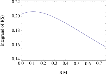
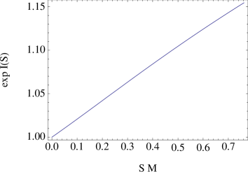
Figure 2: The regularized integrand and its exponentiated integral $\exp I(S)$ ocurring in the integration formula for the isotropic radius $r$, plotted versus $S=1/R$ from $S=0$ to $S_{0}=1/R_{0}\approx 0.762/M$. The resulting effect in $r(R)$ is a factor of order unity that varies monotonically from 1 at $R=\infty$ to $1.155$ at $R=R_{0}$.

Fig. 2 shows numerical results for the integral involved in the calculation of $r(R)$ based on (46) and (67). The main feature is that $\exp I(R)$ varies monotonically and almost linearly between

$$\exp I(R_{0})\approx 1.155,\quad\exp I(\infty)=1.$$ (57)

Considered for $R\rightarrow R_{0}$,

$$\exp I(R)=\exp I(R_{0})\left[1+(R-R_{0})I^{\prime}(R_{0})+\ldots\right],$$ (58)

where $I^{\prime}(R_{0})=-\frac{1}{R_{0}}(1+\frac{a_{2}}{a_{1}^{2}})$ with $a_{1}=\alpha^{\prime}(R_{0})$ and $a_{2}=\alpha^{\prime\prime}(R_{0})$.

Since $\exp I(R)$ is of order unity, $r(R)$ is approximated by

$$r\approx R(1-\frac{R_{0}}{R})^{\gamma}=R^{1-\gamma}(R-R_{0})^{\gamma}$$ (59)

For comparison, the isotropic radius $r_{w}$ of wormhole, fixed-puncture data is given by $R=(1+\frac{1}{2r_{w}})^{2}r_{w}$, or

$$r_{w}=\frac{1}{2}\left(R-1\pm R^{\frac{1}{2}}(R-2)^{\frac{1}{2}}\right).$$ (60)

Apart from the symmetry corresponding to the wormhole, there is some structural similarity to (59), i.e. one could define $\gamma_{w}=\frac{1}{2}$ and $R_{0w}=2$.

For $R\rightarrow\infty$, we have $r\simeq R$, while for $R\rightarrow R_{0}$,

$$r(R) \simeq R^{0.084}(R-R_{0})^{0.916}\exp I(R_{0})$$ (61)

$$\simeq 1.181(R-R_{0})^{0.916},$$

with $r(R_{0})=0$. Therefore, since $\gamma\approx 0.916$ happens to be rather close to unity, and since $\exp I(R_{0})$ is only slowly varying, we expect $r(R)$ to be well approximated by the linear term $(R-R_{0})^{1}$ over the entire range of $R$.

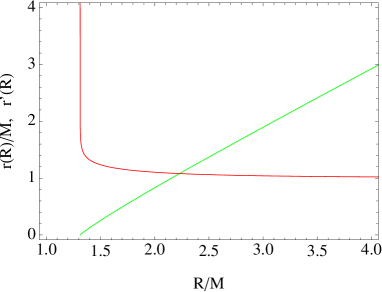
Figure 3: The isotropic radius $r(R)$ and its first derivative $r^{\prime}(R)$. As expected, $r(R)$ is approximately linear for $R$ varying from $R_{0}$ to $\infty$. Its first derivative has a weak pole singularity at $R_{0}$ with exponent $\gamma-1\approx-0.084$.

Fig. 3 shows the quantitative result for $r(R)$, and also for $r^{\prime}(R)$. Since $\gamma<1$, the first derivative has a weak pole singularity at $R_{0}$,

$$r^{\prime}(R)\sim(R-R_{0})^{\gamma-1}\approx\left(\frac{1}{R-R_{0}}\right)^{0.084}.$$ (62)

The same singularity occurs in $r^{\prime}(\alpha)$, the first derivative of $r(\alpha)\sim\alpha^{\gamma}$, see (49). As a quantitative measure of the singularity, we plot (62) in Fig. 4. As another example, $1/x^{0.084}=10$ implies $x\approx 1.1\times 10^{-12}$.

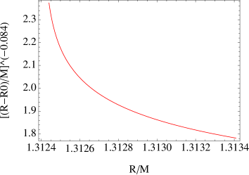
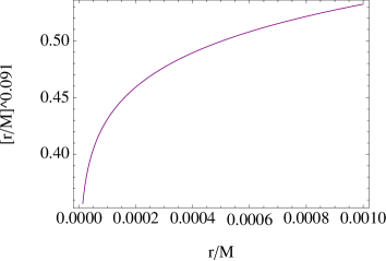
Figure 4: Singular behavior of $(R-R_{0})^{\gamma-1}\approx(R-R_{0})^{-0.084}$ for R in the range from $R_{0}$ to $R_{0}+10^{-3}M$ (top panel), and vanishing of $r^{-1+1/\gamma}\approx r^{0.091}$ near $r=0$ (bottom panel).

A numerical code using isotropic coordinates typically does not compute $r(\alpha)$, but for example

$$\alpha(r)\sim r^{1.091},\quad\alpha^{\prime}(r)\sim r^{0.091},\quad\alpha^{\prime\prime}(r)\sim r^{-0.909}.$$ (63)

If a numerical code relied on $\alpha^{\prime}(0)=0$ at $r=0$, then some inordinate amount of resolution would be required, see Fig. 4. However, typically even $\alpha^{\prime\prime}(r)$ is regularized properly in a standard BSSN moving puncture code due to the factor of $\psi^{-4}\sim r^{2}$ multiplying the second derivative of the lapse in the evolution equations for the extrinsic curvature. The examples (63) show that the lapse is slightly “more regular” at $r=0$ than $\alpha(r)\sim r$.

V Numerics

For various applications of the stationary 1+log slices there remains the task to find numerical solutions for $R(\alpha)$ and $\alpha(R)$, and to compute the integrals of the coordinate transformation to isotropic coordinates to obtain $R(r)$ and $\alpha(r)$. We comment on suitable numerical methods in this section.

V.1 Numerical computation of $R(\alpha)$ and $\alpha(R)$

An explicit form for $R(\alpha)$ is readily obtained based on the roots of a fourth order polynomial, see (26). Implemented in Mathematica, we may have to increase the default working precision for $\alpha$ close to 1, and we have to remove a small complex part of the result at round-off level.

When working outside a package like Mathematica (for concreteness think of an implementation in C or C++), a simpler strategy is to work with a general root finding routine, for example the bracketed Newton method of Press et al. (1992). This allows us to find both $R(\alpha)$ and $\alpha(R)$, as well as inverting other implicit relations, i.e. we typically need such an algorithm anyway. We save the work of implementing the explicit but lengthy formula produced by Mathematica. Newton’s method typically requires only 3 to 6 iterations to reach double precision, taking less time than evaluating Mathematica’s formula (although there are more compact formulas available).

To implement Newton’s method, it is convenient to introduce $S=1/R$, which transforms $R\in[R_{0},\infty)$ to the finite interval $S\in[S_{0},0)$. The integrated 1+log condition gives

$$F(S,\alpha) = \alpha^{2}-1+2S-Ce^{\alpha}S^{4}$$ (64)

$$\frac{\partial F}{\partial S} = 2-4Ce^{\alpha}S^{3}$$ (65)

$$\frac{\partial F}{\partial\alpha} = 2\alpha-Ce^{\alpha}S^{4}$$ (66)

For example, to obtain $S(\alpha)$, fix $\alpha$ and iterate $S$ by Newton’s method for $F(S,\alpha)=0$ with derivative (65). The bracketed Newton method of Press et al. (1992) combines the standard Newton method with a bisection method that is used whenever the Newton step appears to fail, and which in particular avoids that the iteration leaves a given interval. To initialize the method, we have to localize the root approximately, see Fig. 5. Although $S(\alpha)$ and $R(\alpha)$ are monotonic, $F(S,\alpha)$ as a function of $S$ is not. We can bracket the root by setting the starting interval to $[0,S_{c}]$ if $\alpha\in[\alpha_{c},1]$ and to $[S_{c},S_{0}]$ if $\alpha\in[0,\alpha_{c}]$, where $S_{c}=1/R_{c}$. Mathematica’s FindRoot routine applied to the problem requires similar care (i.e. it fails if the root is not bracketed correctly). We also found that Newton’s method works rather well for $R$ on the unbounded interval, for which we can obtain upper and lower bounds for the root from (34). Simple bisection does the job, too, giving on average the expected three digits for ten iterations.

In practice, root finding works well and is applicable for both $R(\alpha)$ and $\alpha(R)$. It can be straightforwardly and efficiently implemented using a simple Newton method Press et al. (1992) (and also with Mathematica’s FindRoot), the only issue being that we have to initialize differently for $\alpha<\alpha_{c}$ and $\alpha>\alpha_{c}$.

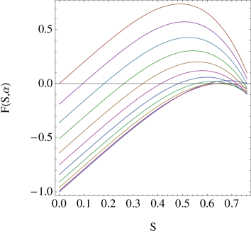
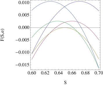
Figure 5: Solving the integrated stationary 1+log condition by root finding. Shown is $F(S,\alpha)$ as a function of $S=1/R$ for $\alpha=0.0$ to $1.0$ in steps of $0.1$ (top panel) and a zoom-in for $\alpha=\alpha_{c}-0.10$ to $\alpha_{c}+0.10$ in steps of $0.05$ (bottom panel). The maximal value of $S$ is $S_{0}\approx 0.762$, the critical value is $S_{c}\approx 0.649$. The solution $S(\alpha)$ is defined by $F(S,\alpha)=0$, and there may be one or two solutions for a given $\alpha$. The root can be bracketed by considering $[0,S_{c}]$ if $\alpha\in[\alpha_{c},1]$ and $[S_{c},S_{0}]$ if $\alpha\in[0,\alpha_{c}]$.

V.2 Numerical integration for isotropic coordinates

Studying the near and far limit of the isotropy condition has left the integrals $I(R)$ or $J(\alpha)$ for numerical evaluation. Although the integrands are regular, at the boundaries they are defined by one-sided limits, which is sometimes called “regular improper” boundaries. In practice it is often sufficient to apply “open” integration formulas, for which the integrands are required close to but not at the boundaries. Accuracy can deteriorate close to an improper boundary, and if this is an issue, Taylor expansions could be used. As already pointed out, if only a numerical answer is required, we can rely on numerical integration routines as available in Mathematica that actually handle improper as well as some types of singular boundaries. In this case the transformation to regular boundaries is not always necessary, cmp. Hannam et al. (2008).

Such routines also handle integrating to $\infty$, as required in $I(R)$. As an alternative, we can change the integration variable to $S=1/R$,

$$I(R)=-\int_{0}^{1/R}\left(\frac{1-\alpha}{\alpha}-\frac{\gamma S}{S_{0}-S}\right)\frac{dS}{S}.$$ (67)

This formula can be directly evaluated using e.g. Romberg integration Press et al. (1992).

The domain of integration in $J(\alpha)$ is finite, but in this case there is a potential issue at $\alpha_{c}$, where the regularity of $R^{\prime}(\alpha)$ relies on the cancellation of roots in the numerator and denominator. For the purpose of integration, split the integral into two pieces as required to handle $\alpha_{c}$ as an improper boundary. (If this is not done explicitly, the Romberg integration routine may place integration points randomly close to $\alpha_{c}$, leading to unexpectedly large errors there.)

When computing initial data in isotropic coordinates, $r(R)$ and $r(\alpha)$ actually still have to be inverted to obtain $R(r)$ and $\alpha(r)$. This can be achieved by root finding similar to what was discussed in Sec. V.1, so we do not discuss this here in further detail.

Integrating (53) as an ODE gives an alternative method to obtain $\alpha(r)$ directly. Examples for useful general purpose integrators are Mathematica’s NDSolve or the Bulirsch-Stoer routine described in Press et al. (1992). From the point of view of using a minimal number of numerical algorithms, the ODE integration can be traded for Romberg integration or whatever else is used to obtain $J(\alpha)$. Also, in this case we can avoid using a root finding routine if we implement $R(\alpha)$ by explicit root formulas. Integrate (53) for $\alpha(r)$ by some ODE algorithm using the explicit root for $R(\alpha)$ on the right-hand-side. Given $\alpha(r)$, compute $R(r)=R(\alpha(r))$ using explicit roots. All other quantities are then directly available in terms of $\alpha(r)$ and $R(r)$.

The issue with integrating an equation for $\alpha(r)$ is that we need a convenient starting point. Both $r=0$ and $1/r=0$ are improper but regular limits. A standard way to proceed is to factor the singularity and use Taylor expansions to integrate away from the boundary. For $\alpha(r)$ (as opposed to $R(r)$), we also have to handle the critical point at $r_{c}$. Note that $r_{c}$ is not directly available, so we cannot start the integration there without, say, performing the explicit integrals discussed above. On the other hand, since accuracy near $r_{c}$ is crucial for a continuous derivative of $\alpha(r)$, starting at $r_{c}$ seems the most promising strategy.

To end with a concrete suggestion, integrate

$$S^{\prime}(r)=-\frac{S(r)\alpha(S(r))}{r}$$ (68)

as an ODE for $S(r)$, letting the automatic step size control of the integrator handle the limits. Compute $\alpha(S)$ by Newton’s method from (64). To avoid issues with starting at improper boundaries, start the integration at

$$r_{c}=0.30345204271479997,\quad S(r_{c})=4(\sqrt{10}-3),$$ (69)

cmp. (22). That is, there is one magic number which we provide for the convenience of the reader based on the explicit integrals, $r_{c}=r(R_{c})$ using Mathematica with 20 digit accuracy. Given $S(r)$, compute $R(r)=1/S(r)$, $\alpha(r)=\alpha(S(r))$ and $f(r)=\psi^{-2}(r)=r/R(r)$.

Independently of how the relation between $r$ and $R$ was obtained, all other quantities required to specify conformally flat initial data in ADM form follow from (10)–(12).

VI Discussion

We have computed the stationary 1+log slices of the Schwarzschild solution in isotropic coordinates. The computation goes beyond what was already known by providing alternative integration methods of the isotropy condition that simplify numerical integration, and by giving direct access to local expansions in the isotropic radius $r$ near $r=0$.

Let us emphasize that the 3D numerical evolutions do not use isotropic coordinates. Specifically, even though $\psi$ is chosen to obtain a metric with uniform determinant, the metric is not diagonal and the conformal metric components can easily deviate by $15\%$ or $20\%$ from $1$. The reason is that although the initial data is conformally flat, there is some significant initial gauge evolution in which e.g. the shift evolves from identically zero to the stationary Gamma-freezing shift. During this time the coordinates are in motion, and the final transformation between the coordinate $r$ and the areal $R$ depends on details of the shift condition and e.g. also the initial value of the lapse. For example, the size of the shift damping parameter $\eta$ directly influences the final gradients in $R(r)$. See Brown (2008); Hannam et al. (2008) for the rather involved procedure to transform the non-isotropic, numerical coordinates to some standard coordinates.

For the analytic stationary 1+log solution in isotropic coordinates, we showed that near the puncture factors of $r$ as well as $r^{1/\gamma}$ play a role. Concretely, $\psi^{-2}\sim r$ and $\beta^{r}\sim r$, while $\alpha\sim r^{1.091}$.

This was not detected in the numerical 3D data since we did not search for a small deviation from $\alpha\sim r^{1.000}$ like $\alpha\sim r^{1.091}$. The main open question in this regard is whether and how much the numerical gauge (which as pointed out is not isotropic) affects these exponents. What are the deviations from isotropy, do they matter at the puncture? In the original ansatz, $g_{ij}=\delta_{ij}+O(r^{2})$, implying that locally at the puncture the coordinates are isotropic. If this holds for arbitrary gauge to leading order, the analysis of isotropic coordinates leading to $\alpha\sim r^{1/\gamma}$ applies also to the numerical simulations.

Furthermore, if stationary 1+log slices in isotropic coordinates are chosen as initial data, then our analysis of the coordinate singularity at the puncture can answer the question what singularity the numerical evolution methods have to handle, if the non-advected Gamma-freezing shift condition is used that preserves the isotropy. The advected Gamma-freezing shift condition leads to different radial coordinates, which in principle could also be analyzed along the lines discussed here for the isotropic case. (See Gundlach and Martin-Garcia (2006); van Meter et al. (2006) for different types of advection in the shift condition using either $\partial_{t}$ or $\partial_{t}-\beta^{i}\partial_{i}$ as time derivative.)

Based on our discussion on integrating the 1+log equation for $\alpha^{\prime}(r)$ in Sec. IV.2, one point to make is that a local Taylor expansion at $r=0$ cannot take into account global boundary conditions or the regularity condition at $\alpha_{c}$. Given any starting value for $R_{0}$ for $r(R_{0})=0$, we can integrate $r^{\prime}(R)$ towards larger $R$, but only specific choices lead to the standard slice (compare Ohme ). For the standard slice, we determine $R_{0}$ from (28) as a function of $C$, which we set to its critical value in (23) based on regularity at $R_{c}$. If we choose a different $R_{0}$, we get a different slice. Expanding the BSSN equations and the gauge conditions near $r=0$ assuming $\alpha\sim r$ rather than $\alpha\sim r^{1/\gamma}$ therefore may well lead to a consistent local solution, which however is incompatible with the global solution we are looking for. More generally, it would be relevant to determine which leading terms of the expansion are independent of global properties. For example, the conformal factor and the shift are linear in $r$ by construction since $\psi^{-2}=\frac{r}{R}$ and $\beta^{r}=\frac{r}{R}\beta$ without any approximation. The leading orders in (2) arise from $R\simeq R_{0}$ and $\beta(R_{0})\simeq\frac{2}{R_{0}}-1$. Only the next to leading order terms involve non-linear $r^{1/\gamma}$ terms.

It is somewhat ironic that the Schwarzschild areal radius (which is not used in 3D numerical simulations) results in a regular Taylor expansion at $R=R_{0}$, while the transformation to isotropic coordinates relabels points such that instead of $r$ the natural variable is $r^{1/\gamma}$. This happens because of the logarithmic nature of the combined 1+log and isotropy conditions. The numerics does not even use isotropic coordinates. Are there globally regular coordinates that remain linear in radius near the puncture?

Part of the motivation to analyze the local properties for $r=0$ in spherical symmetry is to prepare a similar study in axisymmetry. For axisymmetric black holes we do not have an analytic, stationary 1+log solution, but we can write down a Taylor expansion. Axisymmetric moving puncture data include the two important cases of a spinning black hole and of a black hole with linear momentum. Based on numerical experiments, the results for single non-moving punctures generalize to spinning and/or moving punctures, but we do not know yet how this is reflected in a stationary 1+log slice discussion.

The present paper can also be the starting point for the construction of initial data for multiple black holes in the moving puncture gauge since some simplifications and additional details about the analytic single black solution have been obtained. Standard methods superimpose single black hole solutions to obtain an ansatz for the solution of the constraints. In Baumgarte et al. (2009), the conformal thin-sandwich method is considered and the punctures are removed by excision at the apparent horizon. It is demonstrated that stationary 1+log slices for binaries constructed with helical Killing vector boundary are not asymptotically flat (if the data are non-axisymmetric). However, it may still be possible to construct asymptotically flat initial data starting from single moving punctures using a different method.

References

- Campanelli et al. (2006) M. Campanelli, C. O. Lousto, P. Marronetti, and Y. Zlochower, Phys. Rev. Lett. 96, 111101 (2006), eprint gr-qc/0511048.
- Baker et al. (2006) J. G. Baker, J. Centrella, D.-I. Choi, M. Koppitz, and J. van Meter, Phys. Rev. Lett. 96, 111102 (2006), eprint gr-qc/0511103.
- Brandt and Brügmann (1997) S. Brandt and B. Brügmann, Phys. Rev. Lett. 78, 3606 (1997), eprint gr-qc/9703066.
- Beig and O’Murchadha (1994) R. Beig and N. O’Murchadha, Class. Quantum Grav. 11, 419 (1994).
- Beig and O’Murchadha (1996) R. Beig and N. O’Murchadha, Class. Quantum Grav. 13, 739 (1996).
- Dain and Friedrich (2001) S. Dain and H. Friedrich, Comm. Math. Phys. 222, 569 (2001), eprint gr-qc/0102047.
- Misner and Wheeler (1957) C. Misner and J. Wheeler, Ann. Phys. (N.Y.) 2, 525 (1957).
- Brill and Lindquist (1963) D. R. Brill and R. W. Lindquist, Phys. Rev. 131, 471 (1963).
- Hannam et al. (2007a) M. Hannam, S. Husa, D. Pollney, B. Brügmann, and N. Ó Murchadha, Phys. Rev. Lett. 99, 241102 (2007a), eprint gr-qc/0606099.
- Brown (2008) J. D. Brown, Phys. Rev. D77, 044018 (2008), eprint arXiv:0705.1359 [gr-qc].
- Garfinkle et al. (2008) D. Garfinkle, C. Gundlach, and D. Hilditch, Class. Quant. Grav. 25, 075007 (2008), eprint 0707.0726.
- Hannam et al. (2008) M. Hannam, S. Husa, F. Ohme, B. Brügmann, and N. O’Murchadha, Phys. Rev. D78, 064020 (2008), eprint arXiv:0804.0628 [gr-qc].
- Hannam et al. (2007b) M. Hannam, S. Husa, N. Ó Murchadha, B. Brügmann, J. A. González, and U. Sperhake, J. Phys. Conf. Ser. 66, 012047 (2007b), eprint gr-qc/0612097.
- Baumgarte and Naculich (2007) T. W. Baumgarte and S. G. Naculich, Phys. Rev. D75, 067502 (2007), eprint gr-qc/0701037.
- Buchman and Bardeen (2005) L. T. Buchman and J. M. Bardeen, Phys. Rev. D 72, 124014 (2005), eprint gr-qc/0508111.
- (16) F. Ohme, Slicing conditions in spherical symmetry, Diploma Thesis, Universität Jena (2007).
- Brown (2007) J. D. Brown (2007), arXiv:0705.3845 [gr-qc].
- Alcubierre et al. (2003) M. Alcubierre, B. Brügmann, P. Diener, M. Koppitz, D. Pollney, E. Seidel, and R. Takahashi, Phys. Rev. D 67, 084023 (2003), eprint gr-qc/0206072.
- Brügmann (1999) B. Brügmann, Int. J. Mod. Phys. 8, 85 (1999), eprint gr-qc/9708035.
- York (1979) J. W. York, Jr., in Sources of Gravitational Radiation, edited by L. Smarr (Cambridge University Press, Cambridge, 1979), pp. 83–126.
- Baumgarte et al. (2009) T. W. Baumgarte et al., Class. Quant. Grav. 26, 085007 (2009), eprint 0810.0006.
- Bona et al. (1995) C. Bona, J. Massó, E. Seidel, and J. Stela, Phys. Rev. Lett. 75, 600 (1995), eprint gr-qc/9412071.
- Press et al. (1992) W. H. Press, B. P. Flannery, S. A. Teukolsky, and W. T. Vetterling, Numerical Recipes (Cambridge University Press, New York, 1992), 2nd ed.
- Gundlach and Martin-Garcia (2006) C. Gundlach and J. M. Martin-Garcia, Phys. Rev. D 74, 024016 (2006), eprint gr-qc/0604035.
- van Meter et al. (2006) J. R. van Meter, J. G. Baker, M. Koppitz, and D.-I. Choi, Phys. Rev. D 73, 124011 (2006), eprint gr-qc/0605030.
- Cantor (1979) M. Cantor, J. Math. Phys. 20, 1741 (1979).