Gap Solitons and Bloch Waves in Nonlinear Periodic Systems

Abstract

We comprehensively investigate gap solitons and Bloch waves in one-dimensional nonlinear periodic systems. Our results show that there exists a composition relation between them: Bloch waves at either the center or edge of the Brillouin zone are infinite chains composed of fundamental gap solitons(FGSs). We argue that such a relation is related to the exact relation between nonlinear Bloch waves and nonlinear Wannier functions. With this composition relation, many conclusions can be drawn for gap solitons without any computation. For example, for the defocusing nonlinearity, there are $n$ families of FGS in the $n$th linear Bloch band gap; for the focusing case, there are infinite number of families of FGSs in the semi-infinite gap and other gaps. In addition, the stability of gap solitons is analyzed. In literature there are numerical results showing that some FGSs have cutoffs on propagation constant (or chemical potential), i.e. these FGSs do not exist for all values of propagation constant (or chemical potential) in the linear band gap. We offer an explanation for this cutoff.

I introduction

With the state-of-the-art technology, various nonlinear periodic systems have been experimentally realized Lederer ; Morsch . Typical examples include nonlinear waveguide arrays Christodoulides ; Eisenberg , optically induced photonic lattices Fleischer , and Bose-Einstein condensates (BECs) in optical lattices Morsch ; Brazhnyi . In these nonlinear periodic systems, there exist two typical stationary solutions, Bloch waves and gap solitons, which are keys to the understanding of such systems.

Bloch wave is intrinsic to periodic systems Aschcoft . Hence the concept of Bloch wave originally introduced for linear periodic systems can be straightforwardly extended to the nonlinear periodic systems. In both cases, Bloch waves are extensive and spread over the whole space Wu1 . Nonlinearity, however, will significantly affect the stability of Bloch waves. Whence, the analysis of the stability of nonlinear Bloch waves (NBWs) has been a focus of extensive research. For example, the nonlinearity-induced instabilities of Bloch waves are directly responsible for the formation of the train of localized filaments observed in various optical systems Lederer ; Meier2 ; Stepic . For another instance, the instability of Bloch waves has been experimentally observed for BECs in optical latticesBurger ; Fallani , where the instability is closely related to the breakdown of superfluidity in such systemsWu1 ; Smerzi ; Machholm1 .

In contrast, gap solitons are localized in space and only exist in nonlinear periodic systems Lederer ; Christodoulides . So far they have been found to exist in systems of different natures, including nonlinear optical systems Lederer ; Xu ; Sukhorukov ; Cohen ; Meier , BEC systems Louis ; Efremidis ; Pelinovsky , even a surface system Kartashov1 . One particularly important type of gap solitons is fundamental gap solitons (FGSs), whose main peaks are located inside a unit cell Louis ; Efremidis ; Mayteevarunyoo . These FGSs can be viewed as building blocks for the higher order gap solitons Kartashov . We note that other types of localized solutions may also exist for nonlinear periodic systems, such as gap vortex in two-dimensional nonlinear periodic systems Yang . These localized solutions persist in discrete models, where they are called discrete soliton Lederer ; Christodoulides and discrete vortex Malomed , respectively.

A viewpoint has been floating in the community that the NBWs (or higher order gap solitons) can be regarded as chains composed of FGSs in one-dimensional nonlinear periodic systems Alexander ; Carr ; Kartashov ; Smirnov . Such a viewpoint would occur to anyone who has observed the almost perfect match between a NBW and the corresponding FGS as shown in Fig. 1. In particular, Alexander et al. Alexander have found that a new set of stationary solutions, which they call gap waves, can be regarded as the intermediate states between NBW and FGS. This development is a great boost to such viewpoint. However, doubt always lingers as people know that a match between a NBW and the related FGS can be quite bad for a different set of parameters, as shown in Fig. 2(a). Recently, we approached this composition relation from a different angle Zhang . There, we presumed the existence of this composition relation and then investigated how many conclusions could be drawn from it without any computation. These conclusions were eventually verified through numerical computation. In this way, we were able to make a firm claim beyond doubt that the composition relation between NBWs and FGSs exists. Note that a similar relation was pointed out by Carr et al. Carr for extensive periodic solutions and solitons for a nonlinear system without periodic potential.

In this paper we explore in detail this composition relation between NBWs and FGSs Zhang . We not only offer more details on this relationship but also generalize it to the systems with focusing nonlinearity. With this relation one can draw many conclusions without any computation. For example, there are $n$ families of FGSs in the $n$th band gap for the defocusing nonlinearity and the FGS of the $n$th family has $n$ main peaks. All the conclusions will be discussed in detail and be verified with extensive numerical results. Moreover, we have computed the Wannier functions from the NBWs Liang and compared them to the FGSs. We find that these nonlinear Wannier functions match very well with the FGSs. This fact seems to suggest that the composition relation between NBWs and FGSs is related to the exact relation between NBWs and nonlinear Wannier functions. In addition, we have analyzed with different methods the stabilities of the new-found FGSs and the related gap waves Alexander . One method is linear stability analysis; the other is the so-called nonlinear analysis by integrating the dynamic equation with noise Yang . Our numerical results show that not all of these solutions are stable. The stability regions are marked out.

There are numerical results in literature indicating that some FGSs do not exist for all the values of propagation constant (or chemical potential) in the linear band gap Efremidis ; Louis ; Mayteevarunyoo . Namely, there exists a kind of cutoff. Yet it is not clear so far why there is such a cutoff. Here we show that there indeed exists such a cutoff arising from the mixing of different types of FGSs. This mixing can be intuitively viewed as a result of a “chemical reflection”.

This paper is organized as follows. In Sec. II, we give a brief description of our model equation and show how it is related to the concrete systems. In Sec. III, we state the composition relation between NBWs and FGSs and list all the predictions that can be made with this relation. We then demonstrate that all the predictions are valid. In Sec. IV, the FGSs are compared to nonlinear Wannier functions. They resemble each other very well, suggesting that the composition relation is related to the well known relation between Bloch waves and Wannier functions. In Sec. V, the composition relation is applied to construct stationary solutions other than Bloch waves with FGSs, such as gap waves and multiple periodic solutions. In Sec. VI, the stabilities of FGSs and gap waves are examined. In Sec. VII, we offer an explanation why FGSs do not exist for all values of the propagation constant in the linear band gap. Finally, we summarize our results in Sec. IX.

II Model equation

We consider a one-dimensional nonlinear periodic system described by

$$i\frac{\partial\Psi}{\partial{z}}=-\frac{1}{2}\frac{\partial^{2}\Psi}{\partial{x^{2}}}+V(x)\Psi+\sigma|\Psi|^{2}\Psi,$$ (1)

with $V(x)$ being a periodic function. Without loss of generality, we will use $V(x)=\nu\cos(x)$ throughout this paper. The $\sigma$ in Eq. (1) indicates the type of nonlinearity: $\sigma=1$ for the defocusing (or repulsive) case and $\sigma=-1$ for the focusing (attractive) case.

In optics, Eq. (1) describes light propagation along the $z$ direction in the presence of a periodic modulation in $x$ direction. The periodic structure described by $V(x)$ can be experimentally realized with waveguide arrays Christodoulides or optical inducing technology Fleischer . As routinely used in literature, $z$ and $x$ here are respectively scaled to diffractive length and beam width.

In the context of the BEC system, Eq. (1) gives the description of a BEC in the one-dimensional optical lattice with $z$ being the time variable. In such case, Eq. (1) has been scaled as follows: $x$ is in units of $\Lambda/(2\pi)$, $z$ is in units of $\hbar/(8E_{rec})$ and the strength of the optical lattice $v$ is in units of $8E_{rec}$ with $m$ being the atomic mass, $\Lambda$ the period of the lattice and $E_{rec}=\hbar^{2}\pi^{2}/(2m\Lambda^{2})$ the recoil energy.

For stationary solutions in the form of $\Psi(x,z)=\phi(x)\exp(-i\mu{z})$, Eq. (1) is reduced to a $z$-independent equation

$$-\frac{1}{2}\frac{\partial^{2}{\phi}}{\partial{x^{2}}}+\nu\cos(x)\phi+\sigma|\phi|^{2}\phi=\mu\phi.$$ (2)

Here, $\mu$ is referred to as propagation constant in optics. Whereas in the BEC system, $\mu$ represents the chemical potential. In general, NBW and FGS are the two basic types of stationary solutions to Eq. (2). For the FGS which is localized in space, we can define its norm $N$ as

$$N=\int^{\infty}_{-\infty}|\phi(x)|^{2}dx.$$ (3)

By contrast, the NBW spreads over the whole space, hence it is only meaningful to define its averaged norm $\mathcal{N}$ over one period

$$\mathcal{N}=\int^{2\pi}_{0}|\phi(x)|^{2}dx.$$ (4)

The so defined norm is proportional to the laser strength in optics, or the number of atoms for a BEC.

To avoid confusion, hereafter we will present our results and discussions in the framework of optics unless otherwise specified. We first consider the defocusing case, $\sigma=1$.

III Composition relation in the defocusing case

Without the nonlinear term, Eq. (2) is the well-known Mathieu equation Jordan . Its physical solutions are Bloch waves defined by $\phi_{n,k}(x)=\exp(ikx)\psi_{n,k}(x)$ with $\psi_{n,k}(x)=\psi_{n,k}(x+2\pi)$ Aschcoft . Here $k$ is the Bloch wave vector and $n$ is the band index; the $\mu_{n}(k)$ form Bloch bands as $k$ varies through the Brillouin zone (BZ). There exist band gaps between different Bloch bands indexed by $n$, where the physical solutions are forbidden.

With the addition of the nonlinear term, the physical solutions of Eq. (2) become admissible in the linear band gaps. One such typical solution is the gap soliton. Since the propagation constants of gap soliton only take values inside the linear band gaps, no linear counterpart exists for gap soliton. Among various gap solitons, there is a particularly important class called FGSs, whose main peaks locate inside one unit cell.

Figure 1: NBWs (dotted lines) of the first nonlinear band and FGSs (solid lines) in the first linear band gap for $\nu=1.5$ and $\mu=-0.3$. NBW in (a) is at the center of BZ with $\mathcal{N}=1.6908$; NBW in (b) is at the edge of the BZ with $\mathcal{N}=1.6738$.

Figure 2: NBWs (dotted lines) of the first nonlinear band and FGSs (solid lines) in the first linear band gap for $\nu=1.5$. (a) NBW is at the center of BZ with $\mathcal{N}=0.0027$ and $\mu=-0.92$ is near the top of the first linear Bloch band; (b) NBW is at the edge of the BZ with $\mathcal{N}=3.2194$ and $\mu=0.151$ is close to the bottom of the second linear Bloch band.

Despite the nonlinearity, Eq. (2) still admits the Bloch wave solutions. However, the nonlinear term will modify Bloch waves and Bloch bands. For the defocusing case, the nonlinearity not only changes the shapes of the Bloch bands but also moves them up into the linear band gap Wu2 . Here, the strength of nonlinearity is completely described by the norm $\mathcal{N}$. If $\mathcal{N}$ is lowered to zero, these nonlinear bands will move down and be reduced to the linear Bloch bands. When $\mathcal{N}$ is increased, bands will move up continuously without limit.

It is clear from the above discussions that there exist two types of solutions to Eq. (2), NBW and FGS, for a given $\mu$ in the linear band gap. In Fig. 1, we have plotted both NBWs and FGSs for $\mu=-0.3$ in the middle of the first linear band gap. Fig. 1(a) (or (b)) is for a NBW at the center (or edge) of the BZ. In this figure, a nearly perfect match is found between the NBWs and corresponding FGSs inside one unit cell. These numerical results therefore strongly suggest that FGS can be considered as the building blocks for NBWs at either the center or the edge of the BZ. In other words, NBW at the center of the BZ can be viewed as an infinite chain composed of FGSs while NBW at the edge of BZ is built by FGSs with alternative signs.

However, such perfect match does not exist for all $\mu$ in the linear band gaps. After checking various values of $\mu$, we find that the match between the NBW and FGS is very good except in a narrow region near the edge of the linear bands. Two typical results are shown in Fig. 2. Fig. 2(a) is for the case of $\mu$ near the top of the first Bloch band while Fig. 2(b) is for the case of $\mu$ close to the bottom of the second Bloch band. It is evident from Fig. 2(a) that for a $\mu$ close to the edge of the first linear band, the NBW and the FGS does not match well. This mismatch casts strong doubt on the validity of the claim that a NBW can be regarded as an infinite chain composed of FGSs.

In this work, the gap solitons are numerically obtained by using the relaxation method in the coordinate space Mayteevarunyoo ; Kartashov while the Bloch waves are numerically found by applying the relaxation method in the Fourier space Wu2 .

III.1 Direct predictions from the composition relation

We now take a different view at the above observed composition relation between the FGSs and NBWs. We shall first presume the existence of this composition relation and then try to draw as many conclusions as possible. By verifying these conclusions, we will justify this composition relation a posteriori. In this sprit, the following predictions can be immediately drawn without any computation.

(1) For defocusing nonlinearity, there is no FGS in the semi-infinite linear gap below the lowest Bloch band.

As defocusing nonlinearity can be regarded as a result of repulsive interaction, its addition to the system will increase the system energy and therefore move the nonlinear Bloch bands up relative to their linear counterparts. This means that there is no NBW for the $\mu$ in the semi-infinite gap. According to the composition relation, one can then conclude that there is no FGS in the semi-infinite band gap.

(2) There exist $n$ different families of FGSs in the $n$th linear band gap for defocusing nonlinearity.

In order to show this, we have plotted the linear and nonlinear Bloch bands in Fig. 3. Note that all the NBWs in the same nonlinear Bloch band share the same nonlinearity $\mathcal{N}$. As already discussed above, the nonlinearity $\mathcal{N}$ can move the nonlinear Bloch bands up. Therefore, the $m$th nonlinear Bloch band can be lifted into the $n\geq m$ linear band gaps. For example, as $\mathcal{N}$ increases, the first nonlinear Bloch band can be lifted into the first, second, third, and all other linear band gaps. This implies that there exists only one nonlinear Bloch band ( the first nonlinear Bloch band) in the first linear band gap [Fig.3(a)]; two nonlinear Bloch bands (the first and second) in the second linear band gap [Fig.3(b)]; three nonlinear Bloch bands (the first, second, and third) in the third linear band gap [Fig.3(c)]; and so on. In other words, there are $n$ different NBWs in the $n$th linear band gap. NBWs in the different Bloch bands have different characters. With the composition relation, one can immediately conclude that there are $n$ different families of FGSs in the $n$th linear band gap.

In Ref.Wang2 , this rising nonlinear Bloch band by nonlinearity was noted to be useful for analyzing gap waves (or truncated Bloch waves).

Figure 3: Linear and nonlinear (defocusing case) Bloch bands for $\nu=1.5$. Solid lines are linear bands, LB$i$ represents the $i$th linear band. The widthes of linear bands are marked by shadow areas. (a) The first nonlinear Bloch band (dotted line) in the first linear band gap with $\mathcal{N}=1.6908$; (b) the first (dotted) and second (dashed line) nonlinear bands in the second linear band gap with $\mathcal{N}=4.8437$ and $1.5268$ respectively; (c) the first (dotted), second (dashed), and third (dash-dotted line) nonlinear bands in the third linear band gap with $\mathcal{N}=8.3478$, $4.7363$, and $1.0242$ respectively.

(3) In the $n$th linear band gap, the $m$th ($m<n$) family of FGSs exists only above a threshold value of norm $N$ whereas the $n$th family does not have such a value.

Generally, one must increase nonlinearity $\mathcal{N}$ over a critical value to move the $m$th nonlinear Bloch band up into the $n$th ($n>m$) linear band gap while there is no such a critical value to lift the $n$th nonlinear Bloch band into the $n$th linear band gap. An example is shown in Fig. 3(b). In order to lift the first nonlinear band into the second linear band gap, nonlinearity $\mathcal{N}$ must be beyond a threshold value while there is no such a value to move the second nonlinear band into the second linear band gap. This analysis, combined with the composition relation, leads us to predict that there is a threshold value of norm $N$ for the $m$th ($m<n$) family of FGSs in the $n$th linear band gap while the $n$th family have no such a threshold value.

(4) The $n$th family of FGSs has $n$ main peaks inside one unit cell (or an individual well in the periodic potential).

The linear Bloch waves in the $n$th linear Bloch band originate from the $n$th bound state of an individual well of periodic potential. Since the $n$th bound state has $n-1$ nodes, the linear Bloch waves have $n$ main peaks in one unit cell. This character is shared by the Bloch waves belonging to the $n$th nonlinear Bloch band. Therefore, as the building blocks of NBWs, the $n$th family of FGSs should have $n$ main peaks.

Figure 4: NBWs (dotted lines) and FGSs (solid lines) in the second linear band gap for $\nu=1.5$ and $\mu=0.6$. (a) A first-family FGS and its corresponding NBW of the first Bloch band at the center of the BZ with $\mathcal{N}=5.0598$; (b) a first-family FGS and its corresponding NBW of the first Bloch band at the edge of the BZ with $\mathcal{N}=4.8443$; (c) a second-family FGS and its corresponding NBW of the second Bloch band at the center of the BZ with $\mathcal{N}=1.5268$; (d) a second-family FGS and its corresponding NBW of the second Bloch band at the edge of the BZ with $\mathcal{N}=1.7417$.

Figure 5: NBWs (dotted lines) and FGSs (solid line) in the third linear band gap for $\nu=1.5$ and $\mu=1.4$. The solid lines are for FGSs and dotted lines for NBWs. (a,b) A first-family FGS; (c,d) a second-family FGS; (e,f) a third-family FGS. (a,c,e) NBWs at the center of the BZ in the first, second, and third bands with $\mathcal{N}=9.2162,4.7363$, and $2.052$, respectively; (b, d, f) NBWs at the edge of the BZ in the first, second, and third bands with $\mathcal{N}=8.3478,5.6197$, and $1.0242$, respectively.

III.2 Verification of the predictions

In the following, we check the validity of the predictions listed above.

(1) The first prediction is consistent with the well-known and extensively proved fact that gap solitons do not exist in the semi-infinite gap for defocusing nonlinearity Efremidis ; Louis . As a result, this prediction can be considered as the confirmation of a known result.

(2) We resort to the numerical computation to verify the second prediction. As it is impossible to exam every linear band gaps, we foucus on the second and third linear band gaps. We indeed find two families of FGSs in the second linear band gap and three families of FGSs in the third linear band gap. They are shown and compared to the corresponding NBWs in Figs. 4 and 5.

We note that the second family of FGSs are called subfundamental gap solitons in literature Mayteevarunyoo . This indicates that people were not expecting other FGSs to be found. In other words, the existence of the third family of FGSs as shown in Figs. 5 (e) and (f) is a surprise to many. Our results here also show that all the families of FGSs should be regarded equally fundamental as the corresponding NBWs are equally important.

(3) In Fig. 6, we have plotted the $N$ as a function of the $\mu$ for three different families of FGSs. It is clear from the figure that in the second linear band gap the first family of FGSs exists only when their $N>3.4140$ while the second family exists for arbitrary small norm, having no threshold value. In the third linear band gap, the first and second family exist only when their norms $N>8.6105$ and $N>5.0152$, respectively. In contrast, the third family of FGSs has no such threshold value. For comparison, we have also plotted the norms $\mathcal{N}$ of the corresponding NBWs versus $\mu$ in Fig. 6. These NBW norms $\mathcal{N}$ match quite well with the FGS norms $N$.

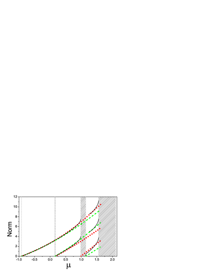
Figure 6: (Color online) Norms of FGSs and NBWs as function of the $\mu$ for $\nu=1.5$. Shaded areas are linear bands. Dotted(red), dashed(green), solid(black) lines represent Bloch waves at the BZ center, Bloch waves at the BZ edge and FGSs respectively.

(4) We have also found that the number of main peaks of a FGS in a well is just what we have expected. In order to demonstrate this clearly, we have plotted Fig. 7 the three families of FGSs in the third linear band gap along with the periodic potential. It is clear that the first family of FGSs has one main peak in an individual well [Fig. 7(a)]; the second and third families of FGSs have two and three main peaks in a unit cell, respectively, as shown in Figs. 7(b) and (c).

Figure 7: Typical profiles of FGSs in the third linear band gap for $\nu=1.5$, and $\mu=1.4$. (a) The first family; (b) the second family; (c) the third family. Dotted lines in the bottom of each figure mimic the periodic potential.

IV Nonlinear Wannier Function and Fundamental gap soliton

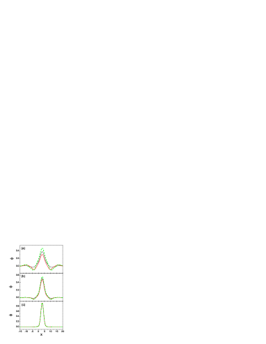
Figure 8: (Color online) Nonlinear Wannier functions for the first nonlinear Bloch band and the corresponding FGSs. Solid (black) lines are for Wannier functions, dashed (green) lines are for the FGSs corresponding to the NBWs at the band edge, and dotted (red) lines are for the FGSs corresponding to the NBWS at the band center. (a) $\nu=0.2$ and $\mathcal{N}=0.5027$; (b) $\nu=0.4$ and $\mathcal{N}=0.7540$; (c) $\nu=1.5$ and $\mathcal{N}=1.6908$.

For a linear periodic system, there is another well-known function, Wannier function, which is localized in space. In one dimension, the Wannier function $W_{n}(x)$ is related to the Bloch wave $\phi_{n,k}$ as follows Aschcoft

$$\phi_{n,k}(x)=\sum_{j}e^{ikx_{j}}W_{n}(x-x_{j})\,,$$ (5)

where $x_{j}$ is the location of the $j$th well in the periodic potential and the summation runs over all potential wells. The relation of Eq. (5) is still valid for nonlinear periodic systems and the corresponding Wannier function can be called nonlinear Wannier function Liang . At either the center or the edge of the BZ, Eq. (5) becomes

$$\phi_{n,\pm}(x)=\sum_{j}(\pm)^{j}W_{n}(x-x_{j})\,,$$ (6)

where $+$ is for the center and $-$ is for the edge. This relation is very similar to the composition relation between NBWs and FGSs that we have just established. Hence, a question naturally arises whether the FGSs bear any relation to the Wannier functions.

In Fig. 5, we have plotted nonlinear Wannier functions and the corresponding FGSs for the first Bloch band together for comparison. The Wannier functions are computed from the Bloch waves in a standard way Liang . For the nonlinearities $\mathcal{N}$ considered here, the first nonlinear Bloch band lies completely in the first linear band gap. As a result, there are two different FGSs for this band, one corresponding to the NBW at the BZ center and the other to the NBW at the BZ edge. Both of the FGSs are plotted in Fig. 5 and are found to match the Wannier functions very well. In fact, the match gets better as the periodic potential gets stronger. Since the Wannier function is normalized, we have scaled them by a factor $\sqrt{N}$ for comparison with the FGSs in Fig. 5.

The excellent match between the FGSs and the Wannier functions suggests that they are related. This relationship may be intuitively understood in the following way. Although a Bloch wave is a solution of a periodic system, the Wannier function is not. In a linear periodic system, any localized wave function, including a Wannier function, will spread in space. In a nonlinear periodic system, it seems that the Wannier function can be modified slightly and become a solution of the system in the form of a FGS.

V Fundamental gap solitons: building blocks for stationary solutions

The composition relation between NBWs and FGSs suggests that the FGSs are really fundamental and can be viewed as building blocks for other stationary solutions to a nonlinear periodic system, such as high-order gap solitons. Our numerical results and existing results in literature Alexander ; Carr ; Kartashov ; Smirnov fully support this view. In the following, we show a few examples.

V.1 Gap waves

Figure 9: Gap waves (solid lines) and the corresponding NBWs (dotted lines) in the third linear gap for $\nu=1.5$ and $\mu=1.4$. The NBWs in (a), (c), and (e) are at the BZ center with $\mathcal{N}=9.2162,4.7363$, and $2.052$ respectively; the NBWs at the BZ edge in (b), (d), and (f) have $\mathcal{N}=8.3478,5.6197$, and $1.0242$ respectively.

In the first example, we construct new solutions by putting finite number of FGSs together. Such solutions are called high order gap solitons in Refs. Kartashov ; Smirnov . There are numerous ways to build these high order gap solitons. For instance, one can use FGSs from different families and put them together with either the same phase or the opposite phase. Here we mainly focus on a class of high order gap solitons called gap waves by Alexander et al. since they can be viewed as truncated NBWs Alexander . For gap waves, all the constituent FGSs come from the same family. These gap waves can be viewed as intermediate states between NBWs and FGSs. With one FGSs, two different classes of gap waves can be constructed. The first class of gap waves, which we call GW-I, are built by putting FGSs side by side similar to the NBW at the center of the BZ. The second class, called GW-II, are composed of FGSs pieced together with alternative signs similar to the NBW at the BZ edge. Some typical gap waves in the third linear band gap and the corresponding NBWs are plotted in Fig. 9. Figs. 9(a), (c), and (e) are GW-I composed of the first, second, and third families of FGSs respectively; Figs. 9(b), (d), and (f) are GW-II. Note that gap waves and the corresponding NBWs have the same propagation constant $\mu$.

We have also plotted gap waves composed of different number of FGSs in Fig. 10 along with the corresponding NBW. The parameters in this figure are the same with ones in Fig. 2(a), where the mismatch between the FGS and the NBW is obvious. Fig. 10 shows an interesting trend that the match between the gap waves and the NBW improves as the number of FGSs increases. This can be viewed as another supporting evidence for the composition relation.

Figure 10: Gap waves composed of different number of FGSs for $\nu=1.5$ and $\mu=-0.92$. Solid lines are for gap waves; dotted line is for the NBW with $\mathcal{N}=0.0027$.

V.2 Multiple periodic solutions

Figure 11: Multiple periodic solutions for $\nu=1.5$, $\mu=-0.1$. (a) period doubled solution; (b) triple periodic solution. Dotted lines are multiple periodic solutions, solid lines are corresponding FGS. Lines in the bottom of each figure mimic periodic potential.

Multiple periodic solutions are extensive states like Bloch waves, but with multiple periods. Mathematically, they are defined as $\phi(x)=\exp(ikx)\psi_{k}(x)$ with $\psi_{k}(x)=\psi_{k}(x+2p\pi)$ and $p>1$ being an integer Machholm .

The composition relation between FGSs and NBWs can be generalized to construct multiple periodic solutions. Here we show two typical kinds of multiple periodic solutions in Fig. 11: one is double periodic solution [Fig. 11(a)]; the other is triple periodic solution [Fig. 11(b)]. The double periodic solution is constructed with the pattern “++- -” and the triple periodic solution is built with the pattern “+++- - -”. One can build other multiple periodic solutions with other patterns. In fact, one can also build the multiple periodic solutions with FGSs from different families. The odd-periodic solutions were speculated to exist in Ref. Machholm .

V.3 Composition relation in the presence of a loop

Figure 12: (a) Loop structure of the first nonlinear band lying in the third linear band gap for $\nu=1$ and $\mathcal{N}/2\pi=1.1344$. Shadow areas are the linear bands and the blank area is the third band gap; (b) NBW (dotted line) for the solid point in (a) with $\mu=1.3$ and the corresponding gap wave (dashed line) and FGS (solid line) in the third band gap.

We have seen in Fig. 3 that all the nonlinear bands move up with the increasing defocusing nonlinearity. It is known that a more dramatic change can happen when the nonlinearity is large enough: loop structures emerge at the BZ edge for the first band and at the BZ center for the second band Wu2 ; Diakonov . The critical value of the nonlinearity for the loop to appear is ${\mathcal{N}}>2\pi\nu$ Wu2 . Our studies show that the composition relation still holds in the presence of such a loop. As an example, we demonstrate this relation for a NBW sitting at the loop top of the first band in Fig. 12. In this figure, the looped nonlinear Bloch band is already in the third linear band gap.

VI stability properties of Fundamental gap solitons and gap waves

Figure 13: Stability of the second family FGS in the second linear gap. (a) Maximum imaginary part of $\delta$ as a function of $\mu$; (b) the eigenvalue plane of $\delta$ at $\mu=0.6$. The inset is the profile of the corresponding gap soliton. $\nu=1.5$.

A question that must be asked for a stationary solution (or a fixed point solution) in a nonlinear system is whether the solution is stable. The unstable solution is very sensitive to small perturbations. The stabilities of the NBWs have been discussed thoroughly in Ref.Wu1 ; Dong . In the following, we shall focus only on FGSs and gap waves.

We use two different approaches to examine the stabilities of the stationary solutions. The first is called linear stability analysis. It is done by adding a perturbation term to a known solution

$$\Psi(z,x)=\Big{[}\phi(x)+\Delta\phi(z,x)\Big{]}\exp(-i\mu z),$$ (7)

where $\Delta\phi(z,x)=u(x)\exp(i\delta z)+w^{*}(x)\exp(-i\delta^{*}z)$ is the perturbation and $\phi(x)$ is the stationary solution. Plugging Eq. (7) into Eq. (1) and keeping only the linear terms, we obtain as follows

$$\begin{pmatrix}\mathcal{L}&-\phi^{2}\\ {\phi^{*}}^{2}&-\mathcal{L}\end{pmatrix}\begin{pmatrix}u\\ w\end{pmatrix}=\delta\begin{pmatrix}u\\ w\end{pmatrix},$$ (8)

with $\mathcal{L}=\frac{1}{2}\frac{d^{2}}{dx^{2}}-\nu\cos(x)-2|\phi|^{2}+\mu$. In Eq. (8), if the eigenvalue $\delta$ has imaginary parts, the solution of $\phi(x)$ is unstable; otherwise, the solution is stable.

In the second method, the perturbed solution in Eq. (7) is used as the initial condition for Eq. (1). Its evolution is then monitored numerically. If its deviation from $\phi(x)$ grows as the system evolves, the solution $\phi(x)$ is unstable; it is stable otherwise. The stability checked by this method is called nonlinear stability Yang .

VI.1 Fundamental gap solitons

Our linear stability analysis shows that the first family of FGSs in the first and second band gaps are stable consistent with Ref. Louis . However, they become unstable in a small area near the band edges in the third gap.

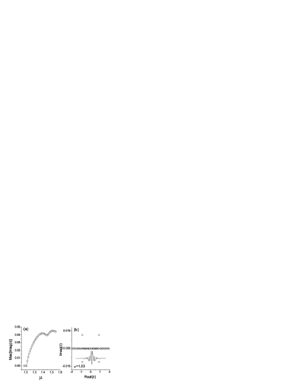
Figure 14: Stability of the third family of FGSs in the third gap. (a) Maximum imaginary part of $\delta$; (b) the eigenvalue plane of $\delta$ at $\mu=1.23$. The inset is the corresponding gap soliton. $\nu=1.5$.

The stability of the second family of FGSs in the second linear band gap is shown in Fig. 13(a), where the stability is measured by the maximum value of the imaginary part of the eigenvalues $\delta$. If the maximum value is zero, the solution is stable; otherwise, it is unstable. It is clear from Fig. 13(a) that this family of FGSs is stable when their $\mu$ are smaller than a critical value near 0.5. For other values of $\mu$ above this critical value, the solitons become unstable. Fig. 13(b) are the eigenvalues for a soliton illustrated in the inset. We see that the eigenvalues $\delta$ are mostly real and become complex only in a very small region. The stability of the third family in the third linear band gap is shown in Fig. 14. The result is very similar to that of Fig. 13 except that the stable region is much smaller. Fig. 14(b) shows an example of the eigenvalue plane.

To double check the stability results, we have propagated perturbed FGSs by numerically solving Eq. (1) with the split-step Fourier method. Gaussian distributed random noise is added to FGSs for the initial wave function. The propagation results shown in Fig. 15 agree with our linear stability analysis. Fig. 15(a) is the propagation of a stable solution while Fig. 15(b) is for an unstable solution.

The above results show that the newly-found third family FGS can be stable and therefore should be observable in experiment. Usually in order to observed gap solitons experimentally, initial input beam profile should be close to the desired soliton profiles Mandelik ; Neshev . We propose to observe the third family FGS using two localized laser beams, whose wavelength is much shorter than the period of a waveguide, to form an interference pattern with three large peaks in a unit cell of the periodic waveguide.

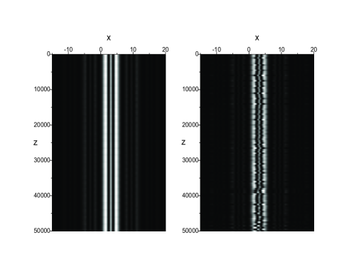
Figure 15: Propagations of gap solitons in the presence of Gaussian distributed random noise with variance $\sigma^{2}=0.01$. (a) Evolution of a third family FGS at $\mu=1.21$ which is stable as indicated by the linear analysis results in Fig.14(a); (b) evolution of an unstable third family FGS at $\mu=1.23$, which is unstable as indicated by the linear analysis results in Fig.14(a) (Max[Imag($\delta$)]=0.0115).

VI.2 Gap waves

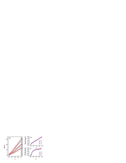
Figure 16: (Color online) Stabilities of gap waves composed of the second family of FGSs in the second gap. (a) the families of gap waves. Circles are for GW-I while triangles for GW-II. Shadow areas are the linear bands; (b) maximum imaginary part of $\delta$ for GW-I; (c) maximum imaginary part of $\delta$ for GW-II.

The stability of gap waves is also analyzed. In general, the GW-I’s corresponding to the first band are stable in the first and second gaps but unstable in the third gap. The stability of gap waves composed of the second family of FGSs in the second gap is shown in Fig. 16. These gap waves contain either 4, 6, or 9 FGSs. These gap waves are characterized by the norms in Fig. 16(a). Fig. 16(b) demonstrates that GW-I are always unstable. GW-II are stable in a small regime near the top of the second band, but they are unstable for other values of $\mu$ as shown in Fig. 16(c). The propagation of the gap waves with noise confirms our stability analysis as shown in Fig. 17. As the three curves fall almost on top of each other in Figs. 16(b,c), we find that the stability of gap waves are independent of how many FGSs they have. Our analysis shows that gap waves other than the types discussed above are unstable.

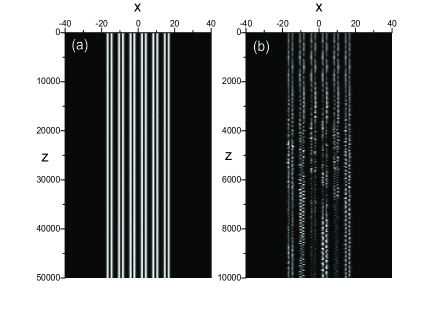
Figure 17: Propagations of gap waves in the presence of a Gaussian distributed random noise with variance $\sigma^{2}=0.01$. (a) propagation of GW-II containing six FGSs at $\mu=0.24$, which is stable indicated by the linear analysis result shown in Fig.16(c); (b) propagation of GW-II with six second family FGSs at $\mu=0.26$, which is unstable as shown in Fig.16 (c) (Max[Imag($\delta$)]=0.0162). Note the different scale of $z$ in (a) and (b).

VII composition relation in the focusing case

We have concentrated on the defocusing case. We now turn to the focusing case. For focusing nonlinearity, Bloch bands and NBWs still exist. Unlike the defocusing case, focusing nonlinearity causes nonlinear bands move down. As a result, the predictions made from the composition relation are different from the defocusing case. (1) There exist infinite number of families of FGSs in the semi-infinite and finite linear band gaps. It is because infinite number of bands can move into a given linear band gap with increasing focusing nonlinearity. (2) In the $n$th linear gap ($n\geq 0$ with $n=0$ for the semi-infinite gap), the $n$th family and other lower order fmailies of FGSs do not exist. (3) In the $n$th linear gap, only the ($n+1$)th family FGSs exist for an arbitrary small values of norm while all other families of FGSs exist only for norms above certain threshold values.

These predictions are confirmed by our numerical computation for the first three bands and the corresponding three band gaps. The results are summarized in Fig.18, where the norms of different FGSs are plotted as functions of $\mu$. As shown in this figure, corresponding to these three bands, there are three families of FGSs in the semi-infinite linear band gap, two families of FGSs in the first linear band gap, and one family of FGSs in the second band gap. In other words, there exist no first family of FGSs in the first linear gap and there exist no first and second families of FGSs in the second gap. Another feature in the figure is the threshold values of norm for some families of FGSs. In the semi-infinite gap, the threshold value for the second family of FGSs is $3.2824$ and for the third family $7.2940$. In contrast, the first family have no such threshold value. In the first gap, the threshold value of norm for the third family of FGSs is $4.0616$ while the second family has no threshold value. The match between the norms of NBWs and FGSs is similar to that in the defocusing case.

Combining with the results for the defocusing case, we have an interesting observation: in the $n$th linear Bloch band gap, the first $n$ families of FGSs exist for the defocusing nonlinearity and the other families ($(n+1)$th, $(n+2)$th, $\cdots$) exist for the focusing nonlinearity.

Figure 18: Norms of fundamental gap solitons as functions of $\mu$ for focusing nonlinearity. Shaded areas are for linear bands; lank areas are for gaps. $\nu=1.5$.

VIII Chemical reflection of FGS

One may have noticed in Figs. 6 and 18 that some families of FGSs do not exist for all values of the $\mu$ in the linear band gaps. For example, in Fig. 6, the second and third families of FGSs in the third linear band gap do not exist for $\mu$ near the edge of third linear Bloch band. The $N$-$\mu$ curves for these two families end at $\mu=1.2658$ and $\mu=1.2612$, respectively, which are away from the right edge of third linear band at $\mu=1.1422$. This cut-off phenomenon was noticed before Alexander . However, to our best knowledge, no one is sure why this cut-off happens. In the following, we show that this cut-off is caused by the mixing of different types of FGSs, which can be intuitively viewed as a result of a “chemical reflection”. It will be discussed for both defocusing and focusing nonlinearities.

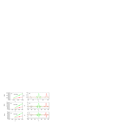
Figure 19: (Color online) Chemical reflection of FGSs into high order gap solitons in the ($N,\mu$) plane for defocusing case with $\nu=1.5$. (a) The $N$-$\mu$ curves for the first family of FGSs in the second gap (solid-red line) and the higher order solitons (dashed-green line) composed of one first-family FGS and two second-family FGSs; (b) the $N$-$\mu$ curves for the first family of FGSs in the third gap (solid-red line) and the solitons (dashed-green line) consisting of one first-family FGS and two third-family FGSs; (c) the $N$-$\mu$ curves for the second family of FGSs (solid-red line) and the solitons (dashed-green line) composed of one second-family FGS and two third-family FGSs. (d, e, f) soliton profiles corresponding to the labeled points in (a, b, c), respectively. Green lines are for profiles of high order solitons, red lines are FGSs, and black lines are profiles of the second family FGS in (d) and the third family FGS in (e) and (f). The lines in the bottom represent periodic potential.

We consider first the defocusing case. We have re-plotted the $N-\mu$ curves (solid lines) in Figs. 19(a,b,c), where the cut-offs exist. In these three figures, we have also plotted the $N$-$\mu$ curves (dashed lines) for three different classes of high order gap solitons. Interestingly, they are connected smoothly to the curves for the FGSs. As illustrated in Figs.19(d,e,f), we find after careful examination that the high order gap solitons for the dashed curve in Fig.19(a) are composed of a first-family FGS sitting in one site and two second-family FGSs sitting in two neighboring sites, the high order solitons in Fig.19(b) composed of a first-family FGS and two third-family FGSs, and the high order solitons in Fig.19(c) consists of a second-family FGS and two third-family FGSs.

To help us understand the turning $N-\mu$ curves, we have developed an intuitive picture to visualize this result. We use the case in Fig. 19(a) as an example. If one imagines an “atom” moving along the lower curve for the FGSs in the ($N,\mu$) plane in Fig. 19(a), this “atom” gets reflected by the “repulsive walls” of the second linear band. Moreover, a “chemical reaction” occurs during the collision between this “atom” of FGS and the “wall”, which may be viewed as a crystal made of “atoms” of the second-family FGS. The result of this reaction is that the “atom” changes its nature to a “molecule” of high order soliton by picking up two second-family FGSs from the second linear band. This “chemical reaction” similarly occurs in Fig. 19(b,c). Based on this intuitive picture, we call this cut-off phenomenon in Figs. 19(a,b,c) chemical reflection.

Note that a similar turning $N-\mu$ curve was also found for gap vortexes in Ref.Wang and gap waves in Ref.Wang2 .

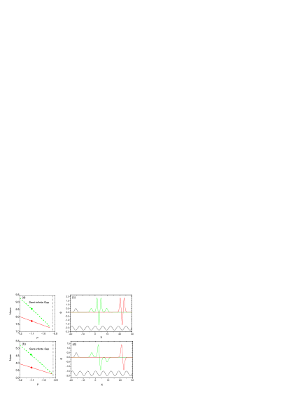
Figure 20: Chemical reflection of the second and third families of FGSs with higher order gap soliton in the semi-infinite gap for focusing case. $\nu=1.5$. (a) the third family of FGSs (solid-red line) and higher order gap solitons (dashed-green line) composted of one third-family FGS and two first-family FGSs. (b) the second family of FGSs (solid-red line) and higher order gap solitons (dashed-green line) composted by one second-family FGS and two first-family FGSs. Dotted lines in (a) and (b) are the first linear band. (c) and (d) soliton profiles corresponding to labeled point in (a) and (b) respectively. Green lines are for profiles of high order solitons, red lines are FGSs, and black lines are profiles of the first family FGS. The lines in the bottom represent periodic potential.

The cut-off phenomenon for the focusing case as shown in Fig. 18 can be similarly be viewed as the result of the chemical reflection. In the focusing case, as shown in Fig. 18, except the lowest family of FGSs in each linear gap, all other families have cut-offs in the propagation constant $\mu$. The cut-off phenomenon can be similarly viewed as the result of the chemical reflection as demonstrated in Fig. 20. Fig. 20(a) is for the third family of FGSs in the semi-infinite gap, whose $N$-$\mu$ curve is found to be connected smoothly to a class of high order gap solitons composed of a third family FGS in one site with two FGSs of the first family in its neighboring sites [see Fig. 20(c)]. The case for the second family of FGSs in the semi-infinite gap is shown in Fig. 20(b), where the high order solitons consist of one FGS of the second family and two FGSs of the first family [see Fig. 20(d)].

IX conclusion

In conclusion, we have demonstrated that a composition relation exists between FGSs and NBWs for both defocusing and focusing nonlinearities. Based on the composition relation, we have drawn many conclusions about the properties of FGSs directly from Bloch band gap structures without any computation. All the predictions have been examined and confirmed. All our studies point to one important conclusion that the FGSs are really fundamental and they serve as building blocks for other stationary solutions in one-dimensional nonlinear periodic systems.

X Acknowledgments

We thank Zhiyong Xu for the helpful discussions. This work was supported by the NSF of China (10825417) and the MOST of China (2005CB724500,2006CB921400). L.Z.X. is supported by the IMR SYNL-T.S. K$\hat{e}$ Research Fellowship.

References

- (1) F. Lederer, G. I. Stegemanb, D. N. Christodoulides, G. Assanto, M. Segev, and Y. Silberberg, Phys. Rep. 463, 1 (2008).
- (2) O. Morsch and M. Oberthaler, Rev. Mod. Phys. 78, 179 (2006).
- (3) D. N. Christodoulides, F. Lederer, and Y. Silberberg, Nature (London) 424, 817 (2003).
- (4) H. S. Eisenberg, Y. Silberberg, R. Morandotti, A. R. Boyd, and J. S. Aitchison, Phys. Rev. Lett. 81, 3383 (1998).
- (5) J. W. Fleischer, M. Segev, N. K. Efremidis, and D. N. Christodoulides, Nature (London) 422,147 (2003).
- (6) V. A. Brazhnyi and V. V. Konotop, Mod. Phys. Lett. B 18, 627 (2004).
- (7) Neil W. Aschcoft and N. David Mermin, Solid state phsyics (Saunders College publishing, 1976).
- (8) Biao Wu and Qian Niu, Phys. Rev. A 64, 061603(R) (2001).
- (9) J. Meier, G. I. Stegeman, D. N. Christodoulides, Y. Silberberg, R. Morandotti, H. Yang, G. Salamo, M. Sorel, and J. S. Aitchison, Phys. Rev. Lett. 92, 163902 (2004).
- (10) M. Stepić, C. Wirth, C. E. Rüer, and D. Kip, Opt. Lett. 31, 247 (2006); C. E. Rüer, J. Wisniewski, M. Stepić, and D. Kip, Opt. Express 15, 6324 (2007).
- (11) A. Smerzi, A. Trombettoni, P. G. Kevrekidis, and A. R. Bishop, Phys. Rev. Lett. 89, 170402 (2002).
- (12) M. Machholm, C. J. Pethick, and H. Smith, Phys. Rev. A 67, 053613 (2003).
- (13) S. Burger, F. S. Cataliotti, C. Fort, F. Minardi, and M. Inguscio, M. L. Chiofalo, and M. P. Tosi, Phys. Rev. Lett. 86, 4447 (2001).
- (14) L. Fallani, L. De Sarlo, J. E. Lye, M. Modugno, R. Saers, C. Fort, and M. Inguscio, Phys. Rev. Lett. 93, 140406 (2004).
- (15) P. J. Y. Louis, E. A. Ostrovskaya, C. M. Savage, and Y. S. Kivshar, Phys. Rev. A 67, 013602 (2003).
- (16) N. K. Efremidis and D. N. Christodoulides, Phys. Rev. A 67, 063608 (2003).
- (17) T. Mayteevarunyoo and B. A. Malomed, Phys. Rev. A 74, 033616 (2006).
- (18) Y. V. Kartashov, V. A. Vysloukh, and L. Torner, Opt. Express 12, 2831 (2004).
- (19) Z. Xu, Y. V. Kartashov, and L. Torner, Phys. Rev. Lett. 95, 113901 (2005).
- (20) A. A. Sukhorukov and Y. S. Kivshar, Opt. Lett. 28, 2345 (2003).
- (21) O. Cohen, T. Schwartz, J. W. Fleischer, M. Segev, and D. N. Christodoulides, Phys. Rev. Lett. 91, 113901 (2003); A. A. Sukhorukov and Y. S. Kivshar, Phys. Rev. Lett. 91, 113902 (2003).
- (22) J. Meier, J. Hudock, D. Christodoulides, G. Stegeman, Y. Silberberg, R. Morandotti, and J. S. Aitchison, Phys. Rev. Lett. 91, 143907 (2003); Z. Chen, A. Bezryadina, I. Makasyuk, and J. Yang, Opt. Lett. 29,1656 (2004).
- (23) D. E. Pelinovsky, A. A. Sukhorukov, and Y. S. Kivshar, Phys. Rev. E 70, 036618 (2004).
- (24) Y. V. Kartashov, V. A. Vysloukh, and L. Torner, Phys. Rev. Lett. 96, 073901 (2006).
- (25) B. Eiermann, T. Anker, M. Albiez, M. Taglieber, P. Treutlein, K. P. Marzlin, and M. K. Oberthaler, Phys. Rev. Lett. 92, 230401 (2004).
- (26) J. Yang and Z. Musslimani, Opt. Lett. 23, 2094 (2003); E. A. Ostrovskaya and Y. S. Kivshar, Phys. Rev. Lett. 93, 160405 (2004).
- (27) B. A. Malomed and P. G. Kevrekidis, Phys. Rev. E 64, 026601 (2001); M. Öster and M. Johansson, Phys. Rev. E 73, 066608 (2006); P. G. Kevrekidis, H. Susanto, and Z. Chen, Phys. Rev. E 74, 066606 (2006).
- (28) L. D. Carr, C. W. Clark, and W. P. Reinhardt, Phys. Rev. A 62, 063610 (2000); 62, 063611 (2000).
- (29) T. J. Alexander, E. A. Ostrovskaya, and Yuri S. Kivshar, Phys. Rev. Lett. 96, 040401 (2006).
- (30) E. Smirnov, C. E. Rüter, D. Kip, Y. V. Kartashov, and L. Torner, Opt. Lett. 32, 1950 (2007).
- (31) Yongping Zhang and Biao Wu, Phys. Rev. Lett. 102, 093905 (2009).
- (32) Z. X. Liang, B. B. Hu and Biao Wu, e-print arXiv:cond-mat/0903.4058.
- (33) D. W. Jordan and P. Smith, Nonlinear Ordinary Differential Equations (Clarendon Press, Oxford, 1977).
- (34) Biao Wu and Qian Niu, New J. Phys. 5, 104 (2003).
- (35) Jiandong Wang, Jianke Yang, Tristram J. Alexander, and Yuri S. Kivshar, Phys. Rev. A 79, 043610 (2009).
- (36) M. Machholm, A. Nicolin, C. J. Pethick, and H. Smith, Phys. Rev. A 69, 043604 (2004).
- (37) D. Diakonov, L. M. Jensen, C. J. Pethick, and H. Smith, Phys. Rev. A 66, 013604 (2002); M. Machholm, C. J. Pethick, and H. Smith, Phys. Rev. A 67, 053613 (2003).
- (38) X. Dong and Biao Wu, Laser Phys. 17, 190 (2007).
- (39) D. Mandelik, R. Morandotti, J. S. Aitchison, and Y. Silberberg, Phys. Rev. Lett. 92, 093904 (2004).
- (40) D. Neshev, A. A. Sukhorukov, B. Hanna, W. Krolikowski, and Y. S. Kivshar, Phys. Rev. Lett. 93, 083905 (2004).
- (41) J. Wang and J. Yang, Phys. Rev. A 77, 033834 (2008).